Three-dimensional simulation of equatorial spread-F with meridional wind effects

www.ann-geophys.net/27/1821/2009/

© Author(s) 2009. This work is distributed under the Creative Commons Attribution 3.0 License.

Annales

Geophysicae

Three-dimensional simulation of equatorial spread-F with

meridional wind effects

J. Krall1, J. D. Huba1, G. Joyce2, and S. T. Zalesak3

1_{Plasma Physics Division, Naval Research Lab., Code 6790, 4555 Overlook Ave., SW, Washington, D.C., 20375-5000, USA} 2_{Icarus Research, Inc., P. O. Box 30780, Bethesda, MD 20824-0780, USA}

3_{Plasma Physics Division, Naval Research Lab., Code 6730, 4555 Overlook Ave., SW, Washington, D.C., 20375-5000, USA} Received: 18 July 2008 – Revised: 23 January 2009 – Accepted: 24 March 2009 – Published: 4 May 2009

Abstract. The NRL SAMI3 three-dimensional simulation code is used to examine the effect of meridional winds on the growth and suppression of equatorial spread F (ESF). The simulation geometry conforms to a dipole field geom-etry with field-line apex heights from 200 to 1600 km at the equator, but extends over only 4 degrees in longitude. The full SAMI3 ionosphere equations are included, provid-ing ion dynamics both along and across the field. The po-tential is solved in two dimensions in the equatorial plane under a field-line equipotential approximation. By selec-tively including terms in the potential equation, the reduced growth predicted by Maruyama (1988) and the stabilization predicted by Zalesak and Huba (1991) are separately real-ized. We find that ESF is stabilized by a sufficiently large constant meridional wind (60 m/s in our example).

Keywords. Ionosphere (Equatorial ionosphere; Ionosphere-atmosphere interactions; Ionospheric irregularities)

1 Introduction

Equatorial spread F (ESF) was first identified by Booker and Wells (1938) as “diffuse echoes from the F-region of the ionosphere received continuously at night in equatorial re-gions over a wide range of wave-frequency” (Booker and Wells, 1938). Despite being first observed 70 years ago and the subject of intense research for the past 35 years (Haeren-del, 1974; Ossakow, 1981; Kelley, 1989; Hysell, 2000), the underlying physical processes that control the onset and non-linear evolution of ESF remain unknown. For example, the

Correspondence to: J. Krall

([email protected])

cause(s) of day-to-day variability of ESF has not been estab-lished (Mendillo et al., 1992; Hysell and Kudeki, 2004; Tsun-oda, 2005, 2006). In this light, ESF continues to be the most perplexing and fascinating ionospheric phenomenon at this time. Additionally, there is a societal impact attendant with ESF: the strong electron-density gradients associated with ESF affect the propagation of electromagnetic signals that can degrade global communication and navigation systems (de La Beaujardiere et al., 2004; Steenburgh et al., 2008).

The possibility that meridional winds could suppress ESF and contribute to the day-to-day variability of ESF has been raised by a number of researchers (Maruyama, 1988; Zalesak and Huba, 1991) based upon theoretical analyses and simpli-fied numerical models. In particular, Maruyama (1988) com-puted the reduced growth rates that result both from redis-tribution of the Pedersen conductivity, along each field line, and from an overall increase in the Pedersen conductance as-sociated with a meridional wind. In Maruyama (1988), the affect of the wind on the background plasma configuration in shown: a trans-equatorial meridional wind tends to push one peak in the Appleton anomaly upwards along the magnetic field and to push the conjugate peak downwards along the field. It is the affect of shifting this latter peak to lower alti-tude and higher neutral densities that increases both the local and the field-line-integrated Pedersen conductivity, reducing the computed ESF growth rate (Maruyama, 1988). In other words, Maruyama (1988) describes an indirect effect of the wind on the instability.

anomaly peaks are shifted, as discussed above in reference to Maruyama (1988), the cross-field wind introduces an ad-ditional non-zero term into the potential equation. Zalesak and Huba (1991) showed that this additional effect can stabi-lize ESF.

Motivated by this work there have been a limited num-ber of observational studies to determine the role of merid-ional winds on the occurrence of ESF, with mixed results. Mendillo et al. (1992) reported results of a two-night study of ESF using the ALTAIR radar and all-sky imaging at Kwajalein. They found that “surges” in the transequatorial winds on relatively short time scales (e.g., few hours to a day) could inhibit the onset of ESF. A subsequent study by Mendillo et al. (2001) during the Multi-Instrumented Stud-ies of Equatorial Thermospheric Aeronomy (MISETA) cam-paign of 1998 found “no convincing evidence that meridional winds at dusk exert a strong influence on ESF onset.” In a study of seasonal variability, Maruyama et al. (2009) find ev-idence for suppression of ESF by meridional winds. New wind and plasma data sets expected from the C/NOFS mis-sion (de La Beaujardiere et al., 2004) are expected to shed light on this issue.

In this study, we apply a recently-developed three-dimensional simulation model of ESF (Huba et al., 2008) to the issue of the partial or complete suppression of ESF by meridional winds. To our knowledge, this is the first com-prehensive modeling study of the impact of meridional winds on the onset and evolution of ESF.

2 SAMI3 simulations

A modified version of the NRL 3-D global ionosphere code SAMI3 (Huba et al., 2008) is used in this analysis. SAMI3 models the plasma and chemical evolution of seven ion species (H+, He+, N+, O+, N+₂, NO+and O+₂). The com-plete ion temperature equation is solved for three ion species

∂Te ∂t −

2 3

1 nek

b2_s ∂ ∂sκe

∂Te

∂s =Qen+Qei+Qphe (4) The various coefficients and parameters are specified in Huba et al. (2000). Ion inertia is included in the ion momentum equation for motion along the geomagnetic field andE×B drifts are computed to obtain motion transverse to the field. Neutral composition and temperature are specified using the empirical NRLMSISE00 model (Picone et al., 2002). The version of SAMI3 used here is modified relative to that used in past studies (Huba et al., 2005) in that the perpendicular electric fieldE⊥=−∇8is used self-consistently in SAMI3

to calculate theE×Bdrifts.

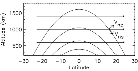
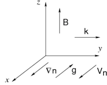
SAMI3 uses a non-orthogonal, irregular grid that con-forms to a model geomagnetic field. For this study the mag-netic field is modeled as a dipole field aligned with the earth’s spin axis, with the result that, in the equatorial plane, the SAMI3 grid is aligned with the coordinate system used in our analysis. For this study, the vertical and zonal neutral winds are set to zero and the meridional neutral wind is set to a constant value. Because the meridional wind crosses field lines, it provides nonzero values both parallel (Vns) and perpendicular (Vnp) to the field as shown in Fig. 1.

The potential equation is derived from current conserva-tion (∇·J=0) in dipole coordinates (s, p, φ). The equation used in this study is

∂ ∂pp6pp

∂8 ∂p +

∂ ∂φ

1 p6pφ

∂8 ∂φ =

∂Fφg ∂φ +

∂FφV

∂φ (5)

where Fφg= −

Z

(rEsin3θ/1)(B0/c)σH cgpds (6) and

FφV = −

Z

(rEsin3θ/1)(B0/c)σPVnpds. (7) Heregpis the component ofgperpendicular toB,

σH c=X i

niec Bi

1

Fig. 2. Contours of electron density plotted in the latitude-altitude

plane for zero wind (upper panel) and 60 m/s (lower panel). These show initial states, before ESF develops.

is the ion component of the Hall conductivity divided by the ion cyclotron frequency,

σP =

X

i niec

B

νin/ i

1+ν_in2/ 2_i

+neec B

νen/ e

1+ν_in2/ 2_i (9) is the Pedersen conductivity, 6pp=R(p1/bs)σPds, 6pφ=R(1/pbs1)σPds,1=(1+3 cos2θ )1/2,i=eB/mic, e=eB/mec, B is the local geomagnetic field, B0 is the geomagnetic field at the equator,bs=(r_E3/r3)1, and rE is the radius of the earth. The field-line integrations above are along the entire flux-tube with the base of the field lines at 85 km. In deriving Eq. (5), we have neglected Hall-conductance terms relative to Pedersen-conductance terms and have neglected∂/∂pterms relative to∂/∂φterms on the right-hand side. Equation (5) is similar to that derived in Haerendel et al. (1992).

2.1 Simulation parameters

The 3-D simulation model is initialized using results from the two-dimensional SAMI2 code. SAMI2 is run for 48 h using the following geophysical conditions: F10.7=170, F10.7A=170,Ap=4, and day-of-year 263 (e.g., 20 Septem-ber 2002). The geographic longitude is 0◦so universal time and local time are the same. The plasma is modeled from hemisphere to hemisphere up to±26◦magnetic latitude; the peak altitude at the magnetic equator is ∼1600 km. The E×B drift in SAMI2 is prescribed by the Fejer/Scherliess

Fig. 3. Contours of Pedersen conductivity plotted in the

latitude-altitude plane for zero wind (upper panel) and 60 m/s (lower panel). These show initial states, before ESF develops.

model (Fejer and Scherliess, 1995). The plasma parameters (density, temperature, and velocity) at time 19:30 UT (of the second day) are used to initialize the 3-D model at each mag-netic longitudinal plane.

The 3-D model uses a grid with magnetic apex heights from 200 km to 1600 km, and a longitudinal width of 4◦(e.g., '460 km) centered at 2◦_{. The grid is(nz, nf, nl)=(101, 130,}

96) wherenzis the number grid points along the magnetic field,nf is the number of “field lines,” andnlis the number in longitude. This grid has a resolution of∼10 km×5 km in altitude and longitude in the magnetic equatorial plane. The grid is periodic in longitude. In essence we are simulating a narrow “wedge” of the ionosphere in the post-sunset pe-riod. Finally, a Gaussian-like perturbation in the ion density is imposed att=0: a peak ion density perturbation of 5% centered at 2◦ longitude with a half-width of 0.25◦, and at an altitudez=400 km with a half-width of 60 km. The seed extends along the entire flux tube.

2.2 Meridional winds effects

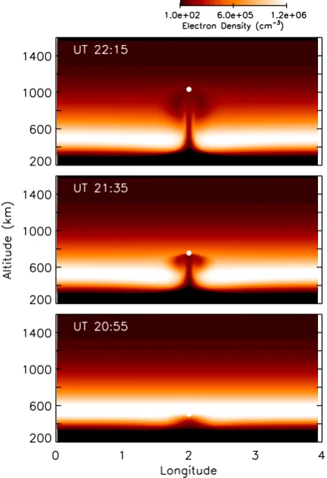
Fig. 4. Contours ofneshowing ESF development with no merid-ional wind.

wind crosses field lines (see Fig. 1), it provides nonzero val-ues both parallel (Vns) and perpendicular (Vnp) to the field. Specifically,Vnsacts through Eqs. (1) and (2), to redistribute the plasma, leading to interhemispheric asymmetries in the electron distribution and the Pedersen conductivity.

In this study, where the winds are northward, the south-ern ionosphere is pushed upwards and the conjugate northsouth-ern ionosphere is pushed downwards. This is illustrated in Fig. 2 where contours of electron density are plotted in the latitude-altitude plane for zero wind (upper panel) and 60 m/s (lower panel). The corresponding effect on the Pedersen conductiv-ity (see Fig. 3) is dramatic. As shown by Maruyama (1988), it is these asymmetries that affect the first term on the right-hand side of Eq. (5) to reduce the growth rate. Below we refer to this as the “indirect” meridional wind effect.

Zalesak and Huba (1991) showed that, in the presence of asymmetric ne and σP distributions, such as shown in Figs. 2 and 3,Vnp acts directly through the∂FφV/∂φ term in Eq. (5) to provide a net stabilizing contribution. For a constant meridional wind, this term is nonzero only if the

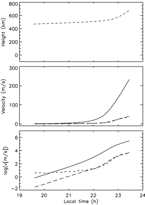
Fig. 5. ESF growth with no meridional wind. Upper: Bubble height

z(dashes) versus time. Middle: Bubble velocitydz/dt(dashes), maximum upward velocityup,max(solid), and maximum

horizon-tal velocityuφ,max(long dashes) versus time. Lower: Log of

ve-locitiesdz/dt (dashes),up,max(solid), anduφ,max(long dashes)

versus time.

interhemispheric plasma distribution is asymmetric. If the wind velocity is large enough, stability results (Zalesak and Huba, 1991). Because all ESF simulations necessarily in-clude the∂Fφg/∂φdriving term, ESF simulations that also include the∂FφV/∂φterm represent both the direct and in-direct meridional wind effects. Below we refer to this as the “full” meridional wind effect.

As shown by Zalesak and Huba (1991) and in the Ap-pendix, these meridional wind effects can be expressed in terms of field-line integrated growth rates:

γ =γg+γ_V, (10)

where γg = −

R

σH c(gp/Ln) ds

R

σPds

(11) and

γ_V = −

R

σP(Vnp/Ln) ds

R

σPds

withL−_n1=∂lnn0/∂pand

σP '

X

i nec

B νin i

σH c '

X

i nec

B 1 i

.

Gravity being directed downwards,gp<0 andγg is always positive (destablizing) in the bottomsideF-layer. Vnp pro-vides both positive and negative contributions (see Fig. 1) with the result thatγ_V is nonzero and negative (stabilizing) so long as the wind acts to shift ne in the direction of the wind as in Fig. 2.

3 Results

The initial condition for each simulation in this study is one in which the F-layer has been lifted to its highest point and is just beginning to fall. We performed several such runs of the SAMI3 code and present cases with constant meridional wind velocities of 0, 20, 40, 50, 60 and 80 m/s. In order to examine the indirect and full wind effects, we selectively ex-clude (indirect effect) or inex-clude (full wind effect) the second term on the right-hand side of Eq. (5).

We first consider the case with zero meridional winds. Figure 4 shows the growth of ESF over a 1.5 h period for no meridional winds. Both terms on the right-hand side of Eq. (5) are included, but have no stabilizing effect on the results. In order to quantify the growth of the instability, we tracked the bubble position, as indicated by the dots in Fig. 4. The dots indicate a position where the density is 80% of its local peak value. We also tracked the maximum upward (up,max) and horizontal (uφ,max) components of the drift ve-locity,u≡E×B.

Figure 5 shows the evolution of the bubble heightz(upper panel, long dashes). Figure 5 (middle panel) shows velocities dz/dt(dashed),up,max(solid), anduφ,max(long dashes). As in Huba et al. (2008), we find peak upward velocities that are much larger than corresponding bubble velocities, indicating the generation of a substantialEfield within the bubble.

Growth times (defined to be the e-folding time 1/γ) can be estimated from the bubble velocitydz/dt or from either component ofu. While each approach produces similar re-sults, the vertical drift velocityup,max gives the most con-sistent result during the early stage of the instability, where the growth is linear. Plots of log(dz/dt ),log(up,max),and log(uφ,max),are shown in Fig. 5 (lower panel). The growth time in this case, obtained via a linear fit to the first 40 min of the log(up,max)curve, is 24.1 min. This growth time is consistent with the 21.6 min growth time reported by Sultan (1996, see Fig. 3a) for no winds and a similar EUV parame-ter (sunspot number 140). As the instability develops nonlin-early, the growth rate increases and computed growth times decrease to match typical observed values of order 15 min.

Fig. 6. Contours ofnefor the 60 m/s “indirect wind effect” case.

3.1 Indirect meridional wind effect

Figure 6 shows the growth of ESF in a case with only the Fφg term of Eq. (5) included and with a steady northward meridional wind of 60 m/s. As in Fig. 4, we tracked the bub-ble position, indicated by dots. Comparison of Figs. 6 and 4 show that the instability has slowed considerably, even dur-ing the nonlinear phase that is shown (in both cases the linear phase begins with a 5% perturbation at 19:30 UT).

Figure 7 shows the evolution of the bubble heightz(upper panel) as well as the bubble velocity dz/dt and peak drift velocitiesup,maxanduφ,max(middle panel). As with Fig. 5, growth times can be estimated from plots of log(dz/dt ), log(up,max), or log(uφ,max), shown in the lower panel. In this case, the “bubble velocity” is initially subject to effects other than ESF, such as the evolution of the background F-layer. Based on a linear fit to the first 40 min of the log(up,max) curve, the growth time is 49.1 min.

Fig. 7. ESF growth in the 60 m/s “indirect wind effect” case.

Up-per: Bubble heightz(dashes) versus time. Middle: Bubble ve-locitydz/dt (dashes), maximum upward velocityup,max (solid),

and maximum horizontal velocity uφ,max (long dashes) versus

time. Lower: Log of velocitiesdz/dt(dashes),up,max(solid), and

uφ,max(long dashes) versus time.

shows plots of∂Fφg/∂φat altitude 415 km, where the driv-ing term was strongest durdriv-ing the linear growth phase of the instability. The driving term is plotted at times 19:30 UT (dashed), 20:15 UT (long dashes) and 21:00 UT (solid) for the zero wind (upper panel) and 60 m/s (lower panel; scale re-duced by a factor of 10) “indirect wind effect” cases. While the driving term is clearly much smaller in the 60 m/s case relative to the zero wind case, it does grow with time. The F-layer remains unstable, albeit with a longer growth time.

Results for these “indirect wind effect” cases (with only theFφv term included in Eq. 5) are summarized in Fig. 9, which shows line plots of log₁₀(up,max)versus local time for no wind (solid), 20 m/s (dashes), 40 m/s (long dashes), 60 m/s (dash-dot), and 80 m/s (lower solid line), with veloc-ities in units of m/s. Clearly the growth of the instability is reduced with rising wind speed, consistent with past results (Maruyama, 1988; Sultan, 1996).

Fig. 8. ESF driving term∂Fφg/∂φat altitude 415 km and at times 19:30 UT (dashed), 20:15 UT (long dashes) and 21:00 UT (solid) for zero wind (upper panel) and 60 m/s “indirect wind effect” (lower panel; scale reduced by a factor of 10).

Fig. 9. Line plots showing log₁₀(up,max)versus local time for no

wind (solid), 20 m/s (dashes), 40 m/s (long dashes), 60 m/s (dash-dot), and 80 m/s (lower solid line) for the “indirect wind effect” runs.

3.2 Full meridional wind effect

Fig. 10. Line plots showing log₁₀(up,max)versus local time for

no wind (solid), 20 m/s (dashes), 40 m/s (long dashes), and 50 m/s (dash-dot), and 60 m/s (lower solid line) for the “full wind effect” runs. Wind velocities differ from those used in Fig. 9.

and with constant meridional wind velocities of 0, 20, 40, 50 and 60 m/s. Results are summarized in Fig. 10, which shows log10(vmax)versus time for each case. Comparing Figs. 9 and 10 shows that, as predicted (Zalesak and Huba, 1991; Sultan, 1996), the instability is stabilized with a sufficiently large meridional wind. In the 60 m/s case, velocities asso-ciated with the initial perturbation simply die down and a quiescent state is obtained.

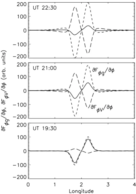
The driving terms∂Fφg/∂φ(dashed) and∂FφV/∂φ(long dashes) are plotted in Fig. 11 for the 60 m/s case, in which ESF was completely stabilized. These are plotted at an altitude of 415 km and at times 19:30 UT (lower panel), 21:00 UT (middle panel), and 22:30 UT (upper panel). This figure shows that, while the individual driving terms increase with time, ∂FφV/∂φ opposes ∂Fφg/∂φ in such a way that the net driving term (solid curve) decreases versus time.

4 Summary

Figure 12 shows that ESF growth times are increased via the indirect wind effect (solid squares) and further increased with the inclusion of the direct wind effect (dots). These results show that the reduced growth predicted by Maruyama (1988) and the stabilization predicted by Zalesak and Huba (1991) are separately realized and that a constant meridional wind of 60 m/s stabilizes spread-F. For comparison to these results, we have computed growth times based on the approximate analytic formulas, Eqs. (10–12). These growth times, shown as open symbols in Fig. 12, are computed for each simulation during ESF linear growth (one hour after each simulation

be-Fig. 11. ESF driving terms∂Fφg/∂φ(dashed) and∂FφV/∂φ(long dashes) at altitude 415 km and at times 19:30 UT, 21:00 UT, and 22:30 UT for the 60 m/s “full wind effect” case. The net driving term is the solid curve in each panel.

gins). We see that the analytic formulas produce reasonable results for low and moderate wind speeds. Above 40 m/s, an-alytic growth times do not vary as strongly with wind speed as was seen in the simulations. For completeness we note that growth times computed using Eqs. (10–12) vary as ESF develops. Typically, a computed growth time exhibits vari-ations of order 10% while the corresponding simulation ex-hibits constant exponential growth.

Fig. 12. Computed growth time (1/γ) versus meridional wind speed for the “indirect wind effect” cases (solid squares) and the “full wind effect” cases (solid circles). Corresponding growth times based on Eqs. (10–12) are shown as open symbols.

the growth time is 52.3 min. Even though thenedistribution shown in Fig. 5b of Sultan (1996) is similar to our 40 m/s case, the Sultan (1996) result features a much larger peak lo-cal wind velocity of 200 m/s. However, it is the asymmetry in the plasma distribution, and the corresponding asymme-try in the Pedersen conductivity, that produces the indirect wind effect (reducing growth) and enables the direct wind effect (further reducing growth and leading to possible stabi-lization). A very large meridional wind is of no consequence without these inter-hemispherical asymmetries. The 60 m/s wind case shown in Figs. 2 and 3 tilts the electron distribu-tion northward to a degree that is clearly greater than that shown in Sultan (1996, Fig. 5b). In other words, our steady 60 m/s wind shows a stronger effect on both the longitude-altitudene distribution and on ESF growth than was found for more realistic wind pattern in which the peak velocity is 200 m/s.

In order to focus on leading-order meridional-wind ef-fects, a number of other phenomena have neglected in this study, such as those associated with zonal winds and those associated with second-order terms in Eq. (5). Specifically Hall-conductance terms were neglected relative to Pedersen-conductance terms and∂/∂pterms were neglected relative to ∂/∂φterms on the right-hand side of Eq. (5). Additional sim-ulations show that the baseline zero-wind case is only min-imally affected when the Hall-conductance and∂/∂pterms are included in the potential equation.

A number of interesting questions have been left for fu-ture study, such as the effect of zonal winds on ESF dynam-ics, the effect of more realistic wind patterns, the determina-tion of the maximum bubble-height for various condidetermina-tions, and the three-dimensional shape and dynamics of the

result-Fig. 13. Slab geometry used in the linear theory.

ing high-altitude depletions. We also have not considered more complex initial perturbations, such as those that lead to bifurcations (Huba et al., 2008), or a higher-order transport scheme that would better capture such physics (see e.g. Huba and Joyce, 2007).

In particular, we have been careful to use similar initial conditions in all cases, with the same specified E×B drift (Fejer and Scherliess, 1995) being used in each case to lift the F-layer prior to the initiation of the self-consistent SAMI3 simulation and with each simulation being initiated at nearly the same local time. Thus, the importance of theE×Bdrift magnitude on these results has not been systematically eval-uated. A study by Mendillo et al. (2001) strongly suggests that ESF growth varies more strongly with the strength of the eastward electric field than with the strength of the merid-ional wind.

We did find that ESF growth is sensitive to the initial state of the F-layer as determined by the ESF initiation time in each simulation. By this, we mean the time at which the imposed drift function used in the SAMI2 initialization is replaced by the self-consistently computed potential and re-sulting drifts of the SAMI3 simulation. For example, ESF simulations initiated at 19:00 local time (equatorial F-layer lifted up to 350 km before initiation of ESF in the zero-wind case) grew about half as quickly as those initiated at 19:30 (F-layer lifted up to 400 km).

5 Conclusions

field. The potential is solved in two dimensions in the equa-torial plane under a field-line equipotential approximation.

By selectively including terms in the potential Eq. (5), the reduced growth predicted by Maruyama (1988) and the sta-bilization predicted by Zalesak and Huba (1991) are sepa-rately realized. Results are summarized in Fig. 12, where the ESF growth times are shown to increase significantly if only the indirect wind effect described by Maruyama (1988) is considered. With the inclusion of all first-order meridional-wind terms in the potential equation, as discussed by Zalesak and Huba (1991), we find that a constant meridional wind of 60 m/s stabilizes ESF. For cases with moderate meridional wind velocities (≤40 m/s) results are consistent with those of Sultan (1996).

Appendix A

Field-line integrated growth rate

We present a heuristic derivation of the generalized Rayleigh-Taylor growth rate given in Eqs. (10–12). We con-sider a slab geometry withB=Bez,g=−gex,Vn=Vnex, andL−_n1=∂lnn0/∂x, wheregis the acceleration due to grav-ity (g>0). The geometry is shown in Fig. 13. Perturbations are taken to vary only as exp[i(ky−ωt )].

The basic equations used in the analysis are the electron continuity equation and current conservation. The electron continuity equation is

∂n

∂t + ∇ ·nVe=0. (A1) Assuming a quasi-equlibrium state so that E=δEey and V_e=δVeex, linearization of Eq. (A1) yields

−iωδn+δVe∂n0

∂x =0. (A2)

Noting thatδVe=(c/B)δEwe obtain c

BδE=iωLn δn n0

. (A3)

The current conservation equation is

Z

∇ ·Jdz=0 (A4)

where the integration is along the magnetic field line and the current is defined by

J =σP

E+B

cVn×eˆz

+σH

_B

cVn−E×eˆz

+

σP i B

c 1

ig+σH i B

c 1

ig×eˆz. (A5)

Here σP = nec

B

"

νin/ i

1+ν_in2/ 2_i

+ νen/ e 1+ν_en2/ 2_e

#

,

σH = nec

B

"

− 1

1+ν2_in/ 2_i

+ 1

1+ν2 en/ 2e

#

,

σP i = nec

B

νin/ i

1+ν_in2/ 2_i,

σH i= nec

B 1 1+ν_in2/ 2_i,

andi=eB/mic. We linearize Eq. (A4) and make use of the local approximation,kLn1, with the result that only the y-component of the current need be retained. This y-component is

δJy=σP

δE−B cVn

+σH iB c

1 i

g. (A6)

Substituting Eq. (A6) into Eq. (A4), making use of Eq. (A3) and takingω=ωr+iγ, we find

Z

δJydz= −γ

Z

σPLn δn n0

B c dz+

Z

σH i δn n0

mi e g dz−

Z

σP δn n0

B

cVn=0. (A7)

Assumingδn/n0is constant along the field line we can solve Eq. (A7) forγ and find that

γ =γg−γV (A8)

where γg =

R

σH i(g/Lni) dz

R

σP dz

and

γ_V =

R

σP(Vn/Ln) dz

R

σPdz .

In the limit where the conductances do not vary along the field line, Eq. (A8) reduces to the standard result

γ = g νinLn

−Vn Ln

, (A9)

where we have here made the F-region approximation, νen/ eνin/ i1, so that σP'(necνin)/(Bi) and σH i'nec/B. Equations (10–12) above represent the gen-eralization of this result to multiple ions.

Acknowledgements. This work was supported by the Office of

Naval Research and NASA.

in the horizontal plasma flow, J. Geophys. Res., 97, 1209–1223, 1992.

Huba, J. D. and Joyce, G.: Equatorial spreadFmodeling: multiple bifurcated structures, secondary instabilities, large density ’bite-outs,’ and supersonic flows, Geophys. Res. Lett., 34, L07105, doi:10.1029/2006GL028519, 2007.

Huba, J. D., Joyce, G., and Fedder, J. A.: SAMI2 (Sami2 is An-other Model of the Ionosphere): A New Low-Latitude Iono-sphere Model, J. Geophys. Res., 105, 23035–23053, 2000. Huba, J. D., Joyce, G., Sazykin, S., Wolf, R., and Shapiro, R.:

Simulation study of penetration electric fields in the low- to mid-latitude ionosphere, Geophys. Res. Lett., 32, L23101, doi: 10.1029/2005GL024162, 2005.

Huba, J. D., Joyce, G., and Krall, J.: Three-dimensional equatorial spreadF modeling, Geophys. Res. Lett., 35, L10102, doi:10. 1029/2008GL033509, 2008.

Hysell, D. L.: An overview and synthesis of plasma irregularities in equatorial spreadF, J. Atmos. Sol. Terr. Phys., 62, 1037–1056, 2000.

Hysell, D. L. and Kudeki, E.: Collisional shear instability in the equatorialF region ionosphere, J. Geophys. Res., 109, A11301, doi:10.1029/2004JA010636, 2004.

variability of equatorial spreadF, J. Geophys. Res., 106, 3655– 3663, 2001.

Ossakow, S. L.: SpreadF theories: A review, J. Atmos. Terr. Phys., 43, 437–452, 1981.

Picone, J. M., Hedin, A. E., Drob, D. P., and Aikin, A. C.: NRLMSISE-00 empirical model of the atmosphere: Statistical comparisons and scientific issues, J. Geophys. Res., 107, 1468, doi:10.1029/2002JA009430, 2002.

Steenburgh, R. A., Smithtro, C. G., and Groves, K. M.: Ionospheric scintillation effects on single frequency GPS, Space Weather, 6, S04D02, doi:10.1029/2007SW000340, 2008.

Sultan, P. J.: Linear theory and modeling of the Rayleigh-Taylor instability leading to the occurrence of equatorial spreadF, J. Geophys. Res., 101, 26875–26891, 1996.

Tsunoda, R.: On the enigma of day-to-day variability in equato-rial spreadF, Geophys. Res. Lett., 32, L08103, doi:10.1029/ 2005GL022512, 2005.

Tsunoda, R.: Day-to-day variability in equatorial spreadF: Is there some physics missing?, Geophys. Res. Lett., 33, L16106, doi: 10.1029/2006GL025956, 2006.