A Theory of Learning with Corrupted Labels
Brendan van Rooyen [email protected]
Robert C. Williamson [email protected]
The Australian National University and Data61 Canberra ACT 2601, Australia
Editor:Inderjit Dhillon
Abstract
It is usual in machine learning theory to assume that the training and testing sets comprise of draws from the same distribution. This is rarely, if ever, true and one must admit the presence of corrup-tion. There are many different types of corruption that can arise and as of yet there is no general means to compare the relative ease of learning in these settings. Such results are necessary if we are to make informed economic decisions regarding the acquisition of data.
Here we begin to develop an abstract framework for tackling these problems. We present a generic method for learning from a fixed, known,reconstructiblecorruption, along with an analyses of its statistical properties. We demonstrate the utility of our framework via concrete novel results in solving supervised learning problems wherein the labels are corrupted, such as learning with noisy labels, semi-supervised learning and learning with partial labels.
Keywords: Supervised Learning, Generalized Supervision, Decision Theory, Minimax Bounds, Data Processing, Noise
1. Introduction
The goal of supervised learning is to find,
arg min
f∈F
E(x,y)∼P`(y, f(x)),
whereF is a hypothesis class of functions and `is loss function. Usually the decision maker is not given direct access toP, but rather a training set comprisingniid samples{(xi, yi)}ni=1 from
P. There are many algorithms for solving this problem, for example empirical risk minimization (ERM), and this problem is well understood.
There are many other types of data one could learn from. For example in semi-supervised learning (Chapelle et al., 2010) the decision maker is given ninstance label pairs andm instances devoid of labels. In learning with noisy labels (Angluin and Laird, 1988; Kearns, 1998; Natarajan et al., 2013), the decision maker observes instance label pairs where the observed labels have been cor-rupted by some noise process. There are many variants including, but not limited to, learning with label proportions (Quadrianto et al., 2009), learning with partial labels (Cour et al., 2011), multiple instance learning (Maron and Lozano-P´erez, 1998) as well as combinations of the above.
c
Abstractly, all of these problems can be understood as corrupted learning problems, in that the “ideal” clean training set is contaminated by a fixed and in general unknown noise process. What is currently lacking is a general theory of learning from corrupted data, as well as means tocompare
the relative usefulness of different data types. Such a theory is required if one wishes to make in-formed economic decisions on which data sets to acquire.
To make progress, we consider abstract prediction problems that have been contaminated by a fixed, known corruption. We demonstrate a generic method for learning from corrupted data, if the corruption isreconstructible. We show the utility of this framework via concrete novel results in supervised learning problems wherein the label has been corrupted, as in learning with label noise, semi-supervised learning and learning with partial labels.
We do not explicitly consider corruption of the instance nor corruption of the label that depends on the instance. While certain examples of these problems are reconstructible, they are not our interest here. We also do not consider non-reconstructible problems such as multiple instance learn-ing/learning with label proportions.
The concrete contributions of this paper are:
• A general method for learning from corrupted labels based on a generalization of the method of unbiased estimators presented in Natarajan et al. (2013) and implicit in the earlier work of Kearns (1998) (theorems 5 and 6).
• Upper and lower bounds on the risk of learning from combinations of corrupted labels, with some analyses of their tightness (theorems 7 and 16). Our results greatly extend the state of the art of Crammer et al. (2005), both in scope and in completeness.
• Demonstration of the computational feasibility of our approach via the preservation of con-vexity (theorem 29).
Elements of our framework have appeared elsewhere, for example in Crammer et al. (2005); Cid-Sueiro et al. (2014); Blanchard et al. (2016); Natarajan et al. (2013). While not the complete story forallproblems, the contributions outlined above make progress toward the final goal of informed economic decisions. The end result is a collection of general tools that allow one tolearn fromand
comparethe usefulness of various corrupted labels.
2. Basic Notation
LetR+be the set of non-negative real numbers. LetYX be the set of functions with domainXand
rangeY. For a setX define the functionsidX(x) =x, and1X(x) = 1. For a functionf ∈RX×Y andy∈Y, we denote thepartialfunctionf(−, y) ∈RX, withf(−, y)(x) =f(x, y), with similar notation for fixing the first argument. We denote the dual spaceof RX, the set of linear maps
RX → R, by(RX)∗. We take the general view that a probability distribution is an element of the dual.
Definition 1 Aprobability distribution on a setX is an element of (RX)∗, i.e. a linear function
1. hP,1Xi= 1.
2. Iff(x)≤g(x), ∀x∈XthenhP, fi ≤ hP, gi.
The linear functionhP,−iis called an expectation. For a large class of general topological spaces, this definition is equivalent to the usual one in terms of measures on sigma algebras (Rudin, 1991). IfXis finite, a distribution is nothing more than a vector.
At times we use the standard prefix notation, withEPf =hP, fi. Define the set of all distributions on a setX to beP(X). For anyx∈ Xdefine the point mass distributionδx, withhδx, fi =f(x) for all functionsf. Finally, for a boolean predicatep :X → {True,False}, let[[p(x)]] = 1ifp(x)
is true and0otherwise. Other notation will be developed as necessary.
3. The General Decision Problem
Consider the problem faced by a scientist in a laboratory. In front of them is a beaker, containing an unknown substance. Available to them are a myriad of experiments that can be performed to ascertain its identity. The scientist could attempt to ignite it, mix a bit of it with a known substance and see what happens, x-ray a sample, throw some of it at high velocity toward an oncoming beam of electrons and so on. Due to time and budget constraints, only a limited number of experiments can be performed to ascertain the substance’s true identity. Therefore the scientist should focus their effort on the “most informative” experiments. Of course, what is informative depends on how the substance is to beused. For example, if the scientist wishes to sprinkle some of it on their food to enhance its flavor, misidentifying arsenic as table salt is a very bad idea. However, if they want to sprinkle it on the snails in their garden, this distinction is less important. The focus of this section is the abstract formulation of this problem. We consider the problem of how a decision maker, or scientist, uses observations from experiments to inform their actions.
Let Θbe a set of possible values of some unknown quantity, and A the set of actions available to the decision maker. The consequence of an action is measured by a loss functionL: Θ×A→R. A negative loss represents a gain to the decision maker. In light of our previous example, Θare the possible substances that could be in the beaker, Ais what the decision maker candowith the substance (eat it, put it on snails and so on), andLmeasures the consequence of an action to the sci-entist (L(arsenic,eat)should be high). The norm of a loss function is given by its largest possible consequence (positive or negative),kLk∞= maxθ,a|L(θ, a)|.
3.1 Transitions
Definition 2 Atransitionfrom a setXto a setY is a linear mapT : (RX)∗ →(RY)∗.
While abstract in appearance, we remark that whenXandY arefinite, a transition is nothing more than amatrix. In general, a transition is an integral operator. Denote the set of all transitions from XtoY byT(X, Y). We call a transitionMarkovifT(P(X))⊆P(Y), ie it maps distributions over Xto distributions overY. WhenXandY are finite, Markov transitions are represented by column stochastic matrices.
Markov transitions constitute a modern approach to conditional probability (Chang and Pollard, 1997; Torgersen, 1991; Le Cam, 1964; Chentsov, 1982). The distribution,
T(x) :=T(δx)
is how the decision maker summarizes their uncertainty aboutY if the true value ofXisx. In fact a transition iscompletely determinedby its value on point masses. Every functionφ∈YX defines a transition with,
hφ(α), fiY :=hα, f ◦φiX, ∀f ∈RY, ∀α∈(RX)∗.
Such a transition is calleddeterministic. Transitions can be combined inseriesand inparallel.
For transitions T ∈ T(X, Y) andS ∈ T(Y, Z)we can define S ◦T ∈ T(X, Z)by usual func-tion composifunc-tion. IfX, Y andZ are finite, then this is just matrix multiplication. IfT andS are Markov, this is just iterated expectation. Intuitively, this can be seen as “marginalizing” overY in the Markov chain,
X→Y →Z.
Combination of transitions in series models corruptions that are performed one after another.
Transitions can be combined in parallel. For α, β ∈ (RX)∗, denote the product by α ⊗β ∈ (RX×X)∗. IfTi ∈T(Xi, Yi),i∈[1;k], are transitions then denote,
⊗ki=1Ti∈T(×ki=iXi,×ki=1Yi) with⊗k
i=1Ti(x) =T1(x1)⊗ · · · ⊗Tk(xk), where×denotes the Cartesian product and⊗denotes products of duals. Transitions can also bereplicated. For any transitionT ∈ T(X, Y)we denote
thereplicated transitionTn∈T(X, Yn), n∈ {1,2, . . .}, with,
Tn(x) :=T(x)⊗ · · · ⊗T(x)
| {z }
ntimes
:=T(x)n,
then-fold product ofT(x).
3.2 Experiments and Risk
Anexperimentis a Markov transitione∈T(Θ,Z). We callZthe observation space of the
exper-iment. The distributione(θ)summarizes uncertainty in the observation whenθis the value of the unknown. After observing the results of an experiment, the decision maker is tasked with choosing a suitable action. They do this via alearning algorithm.
In our language, a learning algorithm is a Markov transitionA ∈ T(Z, A)1. A(z) summarizes the decision makers uncertainty in which action to choose. We define therisk,
RiskL(θ, e,A) :=Ez∼e(θ)Ea∼A(z)L(θ, a) =hA ◦e(θ), L(θ,−)i.
The risk measures the quality of the final action chosen by the decision maker when they use the learning algorithmA, after performing experimente, assumingθis the true value of the unknown. The risk does not provide a single number for the comparison of experiments, rather it provides an entire risk profile. To compare experiments directly we use theminimax risk,
RiskL(e) := inf
A supθ RiskL(θ, e,A),
3.3 The Standard Prediction Problem
The preceding framework for defining and measuring the value of different experiments was largely conceived in the field of theoretical statistics, in the works of von Neumann and Morgenstern (1947); Blackwell (1951); DeGroot (1962) and Le Cam (1964). There is a perceived tension between the goals of statistics, that is todiscoverθ, versus the goals of machine learning, that is topredictthe outcomes of the experimente. As we now show, this distinction is only superficial. Let`:Z ×A→ Rbe a “predictive” loss, that measures how well the actionapredicts the outcome of the experiment e. Common examples include:
ObservationsZ ActionsA Loss`
Density Estimation X⊆Rd ModelΘ⊆P(X) −log(Pθ(x)) Classification X× {±1} Function classF ⊆ {±1}X [[y=f(x)]]
Regression X×R Function classF ⊆RX (y−f(x))2
Supervised Learning X×Y Function classF ⊆P(Y)X `(y, f(x)) Due to the frequency with which we take expectations we overload our notation and define,
`(P, Q) :=Ez∼PEa∼Q`(z, a).
In learning theory,`(P, Q) as defined above is refered to as therisk, here we reserve the termrisk
for its more classical statistical definition. LetΘ =P(Z), the set of all possible distributions on the observation space. The loss functionL:P(Z)×P(A)→Rof interest is theregret,
L(P, Q) :=`(P, Q)− inf
a∈A`(P, a),
Letenbe the experiment that maps eachP ∈P(Z)to itsn-fold productPn. Then,
RiskL(en) = inf
A supP ES∼P
n`(P,A(S))− inf
a∈A`(P, a),
is the minimax regret, a central object in learning theory. Therefore, thepredictionproblem of ma-chine learning can be understood in the more general language of experiments. It is these problems that are of central interest in this paper. For the remainderLwill represent the regret for a loss`.
4. Corrupted Prediction Problems
Due to limitations in the measurement apparatus available to the decision maker, rather than observ-ingz∈ Z, it is often the case that the decision maker observes a corruptedz˜in a potentially different observation spaceZ˜. We model the corruption process via a Markov transitionT ∈T(Z,Z˜).
Definition 3 Acorruptionis a Markov transitionT(Z,Z˜).
For example, we may wish to learn a relationship between measured symptoms and a medical diag-nosis, as provided to us by an expert. To do so, rather than access to the expert’s data, we are given data from one of their apprentices. HereT models the hypothesized link between the expert’s and apprentice’s data. The goal of predicting as well as the expert remains.
More concretely, we are interested in supervised learning problems wherein,
Z =X×Y andZ˜=X×Y ,˜
withT corrupting only the labelY and acting as the identity on the instanceX,
T =idX ⊗TY. Prominent examples include:
• Learning with Label Noise:
TY =
1−σ−1 σ1
σ−1 1−σ1
!
.
• Semi Supervised Learning:
TY =
σ−1 0
0 σ1
1−σ−1 1−σ1
• Learning with partial labels: We assume that a partial label always includes the true label as one of the possibilities and furthermore that spurious labels are added with probabilityσ.
TY =
(1−σ)2 0 0
0 (1−σ)2 0
0 0 (1−σ)2
(1−σ)σ (1−σ)σ 0 (1−σ)σ 0 (1−σ)σ
0 (1−σ)σ (1−σ)σ
σ2 σ2 σ2
For convenience we define the corrupted experimente˜= T ◦e. We order the utility of different corruptions via the minimax risk,
RiskL(˜en) := min
A maxP RiskL(P,e˜n,A). Note that the domain ofAis nowZ˜n. Ideally we wish to compareRisk
L(˜en)withRiskL(en), the minimum risk of the corrupted and the clean experiments. By the general data processing theorem,
RiskL(˜en)≥RiskL(en), however this does not allow one torankthe utility ofdifferentT.
Even after many years of directed research, in general we can not compute RiskL(en) exactly, let alone RiskL(˜en) for general corruptions. Consequently our effort for the remaining turns to upper and lower bounds ofRiskL(˜en).
4.1 Corruption Corrected Losses
When convenient we use the shorthandT(P) = ˜P. Natarajan et al. (2013) introduced a method of learning classifiers from data subjected to label noise, called the “method of unbiased estimators”. Here we show that this method can be generalized to other corruptions.
Recall that a transition T ∈ T(Z,Z˜) is a linear map T : (RZ)∗ → (RZ˜)∗. Associated with
anytransition is adualoradjointlinear mapT∗ :RZ˜ →RZ with, D
α, T∗( ˜f)
E
Z := D
T(α),f˜
E
˜
Z, ∀
˜
f ∈RZ˜, ∀α∈(RZ)∗,
In words,T∗“pulls back” functions of the corrupted sample to functions of the clean sample. When T is a matrix,T∗ is thetransposeofT. We wish to go in the other direction, totransferfunctions of clean samples to those of corrupted samples.
Definition 4 A transitionT ∈T(Z,Z˜)isreconstructibleifT has a left inverse; that is there exists
a transitionR∈T( ˜Z,Z)such thatR◦T = id(RZ)∗.
Intuitively,T is reconstructible if there is some transformation that “undoes” the effects ofT. Note thatRneed not be Markov for Markov T. We denote the set of all reconstructible transitions by
T←(Z,Z˜).
Many forms of corrupted learning are reconstructible, including semi-supervised learning, learn-ing with label noise and learnlearn-ing with partial labels for all but a few pathological cases. Appendix A contains several worked examples.
We call a left inverse ofT areconstruction. For concreteness one can always take,
R= (T∗T)−1T∗,
the Moore-Penrose pseudo inverse ofT. ForinvertibleT, Ris given by the standard inverse. In general it will be useful to consider other reconstructions. In particular, for the proof of theorem 29, we use reconstructions with,
ie those which preserve theconstant loss function. This condition isalways satisfied when T is invertible. More broadly, there is no loss in generality working with such reconstructions.
Reconstructible transitions are exactly those where we can transfer a function of the clean z to one of the corruptedz˜while preserving expectations. By properties of adjoints,
hP, fi=hR◦T(P), fi=hT(P), R∗(f)i.
In words, to take expectations of f with samples fromP˜, we use the corruption corrected f˜= R∗(f). Recall the partial loss function`(−, a) ∈RZ. UsingRwe can reconstruct the partial loss from corrupted examples.
Theorem 5 (Corruption Corrected Loss) For all reconstructible corruptions T ∈ T(Z,Z˜)and
loss functions`:Z ×A→Rdefine thecorruption correctedloss`R: ˜Z ×A→Rwith,
`R(−, a) =R∗(`(−, a)), ∀a∈A.
Then for all distributionsP ∈P(Z),Ez∼P`(z, a) =E˜z∼P˜`R(˜z, a).
4.1.1 USES OFCORRUPTIONCORRECTEDLOSSES INSUPERVISEDLEARNING
In supervised learning Z = X ×Y and the goal is to find a function that predictsy ∈ Y from x∈Xwith low expected loss. Given a suitable function classF ⊆AX and a loss`:Y ×A→ R
one attempts to find,
f∗= arg min
f∈F
E(x,y)∼P`(y, f(x)).
If the labels have been corrupted byTY ∈T(Y,Y˜), we can correct for the corruption and find, f∗= arg min
f∈F
E(x,y˜)∼P˜`RY(˜y, f(x)) = arg min
f∈F
E(x,y)∼P`(y, f(x)).
4.1.2 A WORKEDEXAMPLE: LEARNING WITHSYMMETRICLABELNOISE
When learning under symmetric label noise, the decision maker is required to predict a binary label y ∈ {−1,1}, wherey∼P. Rather than observing the truey, the decision maker observesy˜, where
˜
y =ywith probability1−σandy˜=−ywith probabilityσ. This process can be modeled by the following corruption and reconstruction respectively;
T = 1−σ σ σ 1−σ
!
, R∗ = 1 1−2σ
1−σ −σ
−σ 1−σ
!
.
Note thatRisnotMarkov, as some of the entries ofRare negative. For a loss`:{−1,1} ×A→R
we have,
`R(−1, a) `R(1, a)
!
= 1
1−2σ
1−σ −σ
−σ 1−σ
!
`(−1, a) `(1, a)
!
,
or more compactly,
`R(y, a) =
(1−σ)`(y, a)−σ`(−y, a)
1−2σ .
4.1.3 WHEN TO APPEAL TO ASURROGATELOSS
Many loss functions in machine learning are non convex, the zero one loss a prime example. Rather than minimizing one of these losses directly, it is common to instead minimize a convex surro-gate loss function, such as the hinge loss. When learning in the presence of corruption we face a dilemma; when does one appeal to a surrogate? The method of unbiased estimatorsfirstappeals to a surrogate loss before correcting for noise. The method of label dependent costs (Natarajan et al., 2013) first corrects for noise before appealing to a surrogate.
4.2 Similarities with Other Frameworks
The framework here shares common points with two other broad directions in the literature, in the line of working of Cid-Sueiro et al. (2014) and Blanchard et al. (2016).
Cid-Sueiro et al. (2014); Cid-Sueiro (2012) consider the problem of learning when the corruption is only partially known. They also use transitions (stochastic matrices) and their reconstructions to construct loss functions that “correct for” noise in the labeling process. Their development closely mirrors that of section 11, with subtle differences (see section 11.3).
Blanchard et al. (2016) consider the closely related problem of learning under mutually contam-inated distributions. For example, in binary classification many performance measures can be opti-mized with access to samples fromP1, P−1 ∈P(X), the distribution over instances given a positive
or negative label respectively. In practice however the samples can bemixed, yielding distributions,
˜
P±1 = (1−π±1)P1+π±1P−1.
In general the mixing constants π±1 are unknown. Under the assumption that P1 and P−1 are
mutually irreducible, Blanchard et al. (2016) shows that one can reconstruct the clean distributions
together with the mixing coefficients, providing means to estimate the corruption. Their framework has been extended to other problems (Katz-Samuels and Scott, 2016).
5. Upper Bounds for Corrupted Learning
In this section we develop upper bounds on the risk of any algorithm that learns from a corrupted sample, in terms of thesample risk,S˜∼P˜n. For simplicity we assume thatAis finite. This assump-tion can be removed by PAC-Bayesian bounds (as we do in the appendix), via covering number arguments (Bartlett et al., 1997) or via more refined bounds from empirical process theory (Bartlett and Mendelson, 2006).
By an application of the PAC-Bayes bound (Zhang, 2006), one has for all algorithmsA ∈T( ˜Zn, A) and distributionsP ∈P(Z),
ES˜∼P˜n`R( ˜P ,A( ˜S))≤ES˜∼P˜n`R( ˜S,A( ˜S)) +k`Rk∞ r
2 log(|A|)
n .
Theorem 6 For all reconstructible T ∈ T(Z,Z˜), algorithmsA ∈ T( ˜Zn, A), distributionsP ∈
P(Z)and bounded loss functions`,
ES˜∼P˜n`(P,A( ˜S))≤ES˜∼P˜n`R( ˜S,A( ˜S)) +k`Rk∞ r
2 log(|A|)
n .
A similar result also holds with high probability on draws from P˜n. This bound motivates the following algorithm for learning from corrupted data,
AERM( ˜S) = arg min
a∈A
`R( ˜S, a).
As this algorithm minimizes the loss on the sample,
ES˜∼P˜n`R( ˜S,AERM( ˜S))≤ES˜∼P˜n`R( ˜S, a) =`(P, a), ∀a∈A. Together with theorem 6 we have,
ES˜∼P˜n`(P,AERM( ˜S))≤inf
a `(P, a) +k`Rk∞ r
2 log(|A|) n , ∀P
yielding,
RiskL(˜en)≤ k`Rk∞ r
2 log(|A|)
n .
Similarly,
RiskL(en)≤ k`k∞ r
2 log(|A|)
n .
Therefore, the ratio k`Rk∞
k`k∞ measures the relative difficulty of corrupted versus clean learning, as
judged solely by our upper bound.
5.1 Upper Bounds for Combinations of Corrupted Data
Recall that our final goal is to quantify the utility of a data set comprising different corrupted data. For example in learning with noisy labels out ofndata, there could ben1 clean,n2 slightly noisy
andn3 very noisy samples and so on. More generally we assume access to a corrupted sampleS˜,
made up ofkdifferent types of corrupted data, withS˜i∼P˜ni,i∈[1;k].
Theorem 7 LetTi ∈T(Z,Z˜i)be a collection ofkreconstructible corruptions. LetP˜ =⊗ki=iP˜ ni
i ,
˜ Z = ×k
i=1Z˜
ni
i , n =
Pk
i=1ni andri = nni. Then for all algorithmsA ∈ T( ˜Z, A), distributions
P ∈P(Z)and bounded loss functions`,
ES˜∼P˜`(P,A( ˜S))≤ES˜∼P˜
k X
i=1
ri`Ri( ˜Si,A( ˜S)) +K r
2 log(|A|)
n ,
whereK =
s k P
i=1
A similar result also holds with high probability on draws fromP˜. Theorem 7 is a generalization of the final bound appearing in Crammer et al. (2005) that only pertains to symmetric label noise and binary classification. Theorem 7 suggests the following means of choosingniexamples from each of the corrupted experiments. Letcibe the cost of acquiring data corrupted byTi. First, choose data from theTi with lowestcik`Rik
2
∞until picking more violates the budget constraint. Then choose data from the second lowest and so on.
One must be careful when comparing upper bounds, as there may exist alternate methods for learn-ing from the corrupted sample with better properties. In the next section we present arguments indicating this is not the case.
6. Lower Bounds for Corrupted Learning
Thus far we have developed upper bounds for ERM algorithms. In particular we have found that reconstructible corruption does not affect therateat which learning occurs, it only affects constants in the upper bound. Can we do better? Are these constants tight? To answer this question we develop lower bounds for corrupted learning.
Here we review Le Cam’s method (see Yu (1997) for a more detailed account), a powerful technique for generating lower bounds for decision problems that very often gives the correct rate and depen-dence on constants (including being able to reproduce the standard VC dimension lower bounds for classification presented in Massart and N´ed´elec (2006)). In recent times it has been used to establish lower bounds for: differentially private learning (Duchi et al., 2013), learning in a distributed set up (Zhang et al., 2013), function evaluations required in convex optimization (Agarwal et al., 2012) as well as generic lower bounds in statistical estimation problems (Yang and Barron, 1999). We show how this method can be extended using the strong data processing theorem (Cohen and Kemper-mann, 1998) to provide a general tool for lower bounding the possible performance attainable in corrupted prediction problems.
We stress that these techniques apply to general experimentse ∈ T(Θ,Z), and general loss func-tionsL: Θ×A→R, and not only the predictive problems of interest here.
6.1 Le Cam’s Method and Minimax Lower Bounds
Le Cam’s method proceeds by reducing a general decision problem to an easier binary classification problem, before relating the best possible performance on this classification problem to the minimax risk. LetΘbe a set of unknowns, e ∈ T(Θ,Z) an experiment andL : Θ×A → R a loss. We assume further thatinfaL(θ, a) = 0for allθ∈Θ. Define theseparationρ: Θ×Θ→R,
ρ(θ1, θ2) := inf
a L(θ1, a) +L(θ2, a).
The separation measures how hard it is to act well against bothθ1 andθ2simultaneously.
Further-more define thevariational divergence,
V(P, Q) := sup
f∈[−1,1]Z
The variational divergence measures how hard to is to distinguish two distributionsPandQand is deeply related to binary classification.
Lemma 8 For all experimentse∈T(Θ,Z)and loss functionsL,
RiskL(e)≥ 1
4θ1sup,θ2∈Θ
ρ(θ1, θ2) (1−V (e(θ1), e(θ2))).
A compact proof is given in appendix B. This lower bound is a trade off between distances measured byρand statistical distances measured by the variational divergence. A decision problem is easy if proximity in variational divergence of e(θ1) ande(θ2) (hard to distinguishθ1 andθ2 statistically)
implies proximity ofθ1 andθ2inρ(hard to distinguishθ1andθ2with actions).
Lemma 8 suggests that torank the difficulty of various experiments, one should work with their
Le Cam function.
Definition 9 Letebe an experiment andLa loss. TheLe Camfunction ofeis,
Le CamL(e, γ) =
1
4θ1sup,θ2∈Θ
ρ(θ1, θ2) (1−γV (e(θ1), e(θ2))), ∀γ ≥0.
Lemma 8 can be restated as,
RiskL(e)≥Le CamL(e,1).
REPLICATION ANDRATES
We wish to lower bound how the risk decreases asn, the number of times the experiment is repli-cated, grows. The following lemma provides a simple way to do this.
Lemma 10 For all collections of distributionsPi, Qi∈P(Zi),i∈[1;k],
V(⊗ki=1Pi,⊗ki=1Qi)≤ k X
i=1
V(Pi, Qi).
We make use of the specific case wherePi = P andQi = Qfor alli. Lemma 8 and lemma 10 yield the following.
Lemma 11 For all experimentse∈T(Θ,Z), loss functionsLandn,
RiskL(en)≥Le CamL(en,1)≥Le CamL(e, n).
OTHERMETHODS FOROBTAININGMINIMAXLOWERBOUNDS
6.2 Measuring the Amount of Corruption
Rather than the experimente, in corrupted learning we work with the corrupted experimente˜. The data processing theorem forf-divergences states that,
V(T(P), T(Q))≤V(P, Q), ∀P, Q∈P(Z).
Thus any lower bound achieved by Le Cam’s method forecan be directly transferred to one for
˜
e. However, this provides us with no means to rank differentT. For someT, the data processing theorem can bestrengthened.
Definition 12 TheClarityof a Markov transitionsT ∈T(Z,Z˜)is,
Clarity(T) := sup
P,Q∈P(Z)
V(T(P), T(Q)) V(P, Q) .
One has,
V(T(P), T(Q))≤Clarity(T)V(P, Q), ∀P, Q∈P(Z).
Clarity(T) measures how muchT corrupts. For example, ifT is constant and maps allP to the same distribution, thenClarity(T) = 0. IfT is an invertible function, thenClarity(T) = 1. When
ZandZ˜are finite,
Clarity(T) = sup
v∈Ω
kT(v)k1 kvk1 ,
whereΩ = {v:P
vi = 0, v 6= 0}. HenceClarity(T)is the operator 1-norm ofT when restricted toΩ.Claritybehaves as expected under composition.
Lemma 13 For all transitionsT1 ∈T(Z,Z˜1)andT2 ∈T( ˜Z1,Z˜2),
Clarity(T2◦T1)≤Clarity(T2)Clarity(T1)≤min(Clarity(T2),Clarity(T1)).
HenceT2◦T1is at least as corrupt as either of theTi.
Clarity(T)was first used by Dobrushin (1956), where it is called the coefficient of ergodicity and is used to prove rates of convergence of Markov chains to their stationary distribution.
6.3 Lower bounds Relative to the Amount of Corruption
Together with lemma 11, theClarityleads to meaningful lower bounds that allow the comparison of different corrupted experiments.
Theorem 14 For all experimentse, loss functionsL, corruptionsT ∈T(Z,Z˜)andγ ≥0,
Le CamL(T ◦e, γ)≥Le CamL(e,Clarity(T)γ).
The proof is a simple application of the strong data processing theorem. Together with lemma 11, the above lemma yields the following corollary.
Corollary 15 For all experimentse, loss functionsL, corruptionsT ∈T(Z,Z˜)andn,
In particular if Le Cam’s method yields a lower bound of √C
n for the clean problem, as is usual for many machine learning problems, theorem 15 yields a lower bound of√ C
Clarity(T)nfor the corrupted problem. Therateat which one learns is unaffected, only the constants. A penalty ofClarity(T)is unavoidable no matter what learning algorithm is used.
6.4 Lower Bounds for Combinations of Corrupted Data
As in section 5.1 we present lower bounds for combinations of corrupted data. For example in learning with noisy labels out ofndata, there could ben1clean,n2slightly noisy andn3very noisy
samples and so on.
Theorem 16 LetTi∈T(Z,Z˜i),i∈[1;k], bekcorruptions. LetT =⊗ki=1T
ni
i withn=
Pk
i=1nk.
Then,
Le CamL(T◦en, γ)≥Le CamL e, n X
i=1
niClarity(Ti) !
γ
!
.
Furthermore,
RiskL(T ◦en)≥Le CamL e, n X
i=1
niClarity(Ti) !!
.
As in section 5.1, this bound suggests means of choosing data sets via the following integer program,
arg max
n1,n2...nk
k X
i=1
Clarity(Ti)ni subject to k X
i=1
cini≤C,
where ci is the cost of acquiring data corrupted byTi andC is the maximum total cost. This is exactly the unbounded knapsack problem (Dantzig, 1957) which admits the following near optimal greedy algorithm. First, choose data from theTiwith highest Clarity(ci Ti) until picking more violates the constraints. Then pick from the second highest and so on.
6.5 The Generality of Clarity
In light of section 6.1, it is often the case that more complicated lower bounding techniques based on pairwisef-divergences are required to produce tightlower bounds. Recall the definition of an f-divergence (Ali and Silvey, 1966).
Definition 17 Letf : R+ → Rbe a convex function withf(1) = 0. For all distributionsP, Q ∈ P(Z)thef-divergencebetweenP andQis,
Df(P, Q) :=EPf
dQ dP
,
ifP andQareabsolutely continuous, and is infinite otherwise.
Both the variational and KL divergence are examples of f divergences. Following on from the reasoning of section 6.2, we seek aClarityf(T)such that,
Df(T(P), T(Q))≤Clarityf(T)Df(P, Q)∀P, Q, f.
Theorem 18 (Strong Data Processing(Theorem 4.1 of Cohen et al. (1993))) Let T ∈ T(Z,Z˜)
be a Markov transition. Then for allP, Q, f,
Df(T(P), T(Q))≤Clarity(T)Df(P, Q).
7. Measuring the Tightness of the Upper Bounds and Lower Bounds
In the previous sections we have shown upper bounds that depend onk`Rk∞as well as lower bounds that depend onClarity(T). Here we compare these bounds.
Recall from theorem 5, `R(−, a) = R∗(`(−, a)). The worst case ratio k`k`kRk∞∞ is determined by
theoperator normofR∗. For a linear mapR:RX →RY define,
kRk1:= sup
v∈RX
kRvk1 kvk1
andkRk∞:= sup v∈RX
kRvk∞
kvk∞
which are two operator norms ofR. They are equal to the maximum absolute column and row sum ofRrespectively (Bernstein, 2009). HencekRk1 =kR∗k∞.
Lemma 19 For all losses`,T ∈T(Z,Z˜)and reconstructionsR, k`Rk∞
k`k∞ ≤ kR
∗k ∞.
Lemma 20 IfT ∈T(Z,Z˜)is reconstructible, with reconstructionR, then,
1
Clarity(T) ≤1/
inf
u∈RX
kT uk1 kuk1
≤ kR∗k∞.
Note that for lower bounds we look at thebestcase separation of columns ofT, for upper bounds we essentially use theworst. We also get the following compositional theorem.
Lemma 21 If T1 ∈ T(Z,Z˜1)and T2 ∈ T( ˜Z1,Z˜2) are reconstructible, with reconstructionsR1
andR2, thenT2◦T1is reconstructible with reconstructionR1◦R2. Furthermore,
1
Clarity(T1)Clarity(T2)
≤ kR1◦R2k1 ≤ kR1k1kR2k1.
Proof The first statement is obvious. For the first inequality simply use lemma 20 followed by lemma 13. The second inequality is an easy to prove property of operator norms.
7.1 Comparing Theorems 6 and 15
We have shown the following implication,
C1 √
n ≤RiskL(en)≤
C2k`k∞
√
n ⇒
C1
p
Clarity(T)n ≤RiskL(˜en)≤
C2k`Rk∞
√
n ,
factor ofpClarity(T)apart. We do not know if this is the fault of our upper or lower bounding techniques. However, forspecific`andTthis gap can be smaller.
For example, in the problem of learning with symmetric label noise discussed in section 4.1.2, with misclassification loss`01,
Clarity(T) = 1−2σ and k`01,Tk=
1−σ 1−2σ,
respectively. The worst case ratio of upper and lower bounds over all losses is of order √ 1
1−2σ. For misclassification loss the actual ratio is √1−σ
1−2σ. For allσ ∈ [0,
2
10], i.e. up to0.2flip probability,
this ratio is never larger than √4
15 ≈1.03. 7.2 Comparing Theorems 7 and 16
LetCost(T)be the cost of acquiring data corrupted byT. Theorem 7 prefers corruptions with low
k`Rk2∞Cost(T), or equivalently those with high,
1 k`Rk∞Cost(T) Theorem 16 prefers corruptions with high,
Clarity(T) Cost(T) ≈
k`k∞
k`Rk∞Cost(T) .
In theorems 16 and 7 we have, respectively, best case and a worst case loss specific method for choosing data sets. Theorem 7 combined with 1emma 19 provides a worst case loss insensitive method for choosing data sets.
8. Corrupted Learning when Clean Learning is Fast
The contents of this paper largely solve the problem of learning from data with corrupted labels, when learning on the original problem occurs at thestandard √1
n rate. There are many conditions under which clean learning is fast, here we focus on the Bernstein condition presented in Bartlett and Mendelson (2006); van Erven et al. (2012).
Definition 22 LetP ∈P(Z),`a loss andaP = arg minaEz∼P`(z, a). A pair(`, P)satisfies the Bernstein conditionwith constantKif for alla∈A,
Ez∼P(`(z, a)−`(z, aP))2 ≤KEz∼P`(z, a)−`(z, aP)
WhenAis finite, such a condition leads to n1 rates of convergence for empirical risk minimization (ERM).
Theorem 23 LetAbe ERM withAfinite. If(`, P)satisfies the Bernstein condition then for some
constantC >0,
ES∼Pn`(P,A(S))−`(P, aP)≤ Clog(
|A|)
Furthermore with probability at least1−δon a draw fromPnone has,
`(P,A(S))−`(P, aP)≤
C log(|A|) + log 1δ
n .
While our lower bounding techniques will turn a lower bound of n1 for clean learning to one of
1
α(T)n for corrupted learning, it may be the case that this bound is too optimistic, there may be no algorithm that gives an1 rate of convergence.
A natural question to ask is when using the ERM algorithm for the loss`Rconverges quickly from samples drawn fromP˜. Here we ask the simpler question: when does(`R,P˜)satisfy the Bernstein condition?
Lemma 24 If (`R,P˜) satisfies the Bernstein condition with constantK then (`, P) also satisfies
the Bernstein condition with the same constant.
This theorem (almost) rules out pathological behavior where ERM learns quickly from corrupted data and yet slowly for clean data. The converse of lemma 24 is not true, for example consider the case of PAC learning versus PAC learning with arbitrary instance dependent noise. In some cases the Bernstein condition can be transfered from the clean problem to the corrupted problem, as we now explore.
Definition 25 LetT ∈T(Z,Z˜)be a corruption and`a loss. A pair(`, T)areη-compatibleif for
allz∈ Z anda1, a2 ∈A,
Ez˜∼T(z)(`R(˜z, a1)−`R(˜z, a2))2 ≤η(`(z, a1)−`(z, a2))2.
Theorem 26 If the pair(`, P)satisfies the Bernstein condition with constantKand the pair(`, T)
areη-compatible then(`R,P˜)satisfies the Bernstein condition with constantηK.
While by no means the final word on fast corrupted learning, this theorem does allow one to prove interesting results in the binary classification setting.
Theorem 27 Let T be label noise, T = 1−σ−1 σ1 σ−1 1−σ1
!
, then the pair (`01, T) is η
-compatible withη=
1+|σ−1−σ1|
1−σ−1−σ1
2
.
One very useful example of a pair(P, `)satisfying the Bernstein condition with constant1is when P is separable, `is01loss and the Bayes optimal classifier is in the function class. Theorem 27 guarantees that as long asσ−1+σ1 6= 1(i.e. it is possible to learn from noisy labels), one learns at
9. Canonical Losses and Convexity
Thus far we have focused on the statistical properties of corrected loss minimization procedures. However, performing our correction may incur a computational penalty. Even if the loss`is con-vex, there is no guarantee that the corrected loss remains so. Here we show that a large and useful class of loss functions remain convex when corrected.
Recall the constant function,1Z(z)and define,
1⊥Z := (
v∈RZ :X
z∈Z
v(z) = 0
)
,
those functions that are orthogonal to 1Z. Proper losses and the closely related canonical losses form a large class of loss functions that provide means of attacking prediction problems.
Definition 28 A lossL:Z ×A→RiscanonicalifAis a convex subset of1⊥Z and,
L(z, v) =− hδz, vi+ Ψ(v),
for some convex functionΨ :A→R.
Intuitively, minimizing a canonical loss reduces to “lining up” with the average observed label, with “over confident” predictions penalized by the function Ψ. In appendix C we show that all losses are essentially canonical losses in disguise (theorem 49). Note that canonical losses split into two terms, one convex invand unaffected by the observation, and a term linear inv. These losses are particular easy to correct for corruption, as only the linear term needs to be corrected.
Theorem 29 (Correcting Canonical Losses) LetL : Z ×A → R be a canonical loss. For all
reconstructible corruptionsT ∈T(Z,Z˜)there exists a reconstructionRsuch that,
LR(˜z, v) =− hδz˜, R∗(v)i+ Ψ(v)
FurthermoreRcan be calculated efficiently via Gaussian elimination.
We develop the necessary representation results needed to prove this theorem in appendix C.
Theorem 29 extends results presented in Natarajan et al. (2013) concerning when losses used for learning binary classifiers remain convex when corrected for asymmetric label noise. Therefore we need not abandon the framework of convex surrogates when the corruption is known.
9.1 Comparison with Natarajan et al. (2013)
Recall in the problem of learning with label noise,
T = 1−σ−1 σ1 σ−1 1−σ1
!
whereσy is the probability of labelybeing flipped. For this problem, the corrected loss is,
`R(y, a) =
(1−σ−y)`(y, a)−σy`(−y, a)
1−σ−1−σ1
.
If`:{±1} ×R→Ris convex, smooth and satisfies, `00(y, a) =`00(−y, a),
then lemma 4 of Natarajan et al. (2013) guarantees that`Ris convex. Integrating twice yields,
`(y, a) =by+cyv+g(a),
For some convex functiong. Rearranging one has,
`(y, a) =
b−1−b1+ (c1−c−1)a 2
y+b1+b−1+ (c1+c−1)a
2 +g(a)
| {z }
convex ina
.
For canonical losses, corollary 50 states that any binary canonical loss is of the formL:{±1}×I → R,
L(y, v) =−yv+ Ψ(v), v∈I,
whereI is a convex subset ofRandΨ :I →Ra convex function. Letting,
ν =−
b−1−b1+ (c1−c−1)a 2
,
one can see that the losses considered in Natarajan et al. (2013) are affine re-parametrizations of canonical losses. Theorem 29 is therefore a generalization of lemma 4 of Natarajan et al. (2013).
9.2 Comparison with Cid-Sueiro et al. (2014)
Section 5 of Cid-Sueiro et al. (2014) provides some discussion of the convexity of corruption cor-rected losses. They state, without proof, that a requirement for the preservation of convexity is that the reconstruction havenon negativeentries. Theorem 29 shows that this is not the case, one
canalwayspreserve convexity as long as the correct reconstruction and parametrization of the loss
function are used.
10. Learning when the Corruption Process is Partially Known
Thus far we have considered the problem of learning when T is known. Here we consider the problem of whenT lies in a subset C ⊂ T←(Z,Z˜). For example when learning classifiers under symmetric label noise (Angluin and Laird, 1988), the corruption is of the form,
Tσ =
1−σ σ
σ 1−σ
!
,
If we assume access to a “gold standard” sampleS∼Pnas well as a corrupted sample S˜, we can use methods akin to those in Kearns (1998). One covers the setCto some tolerancewith a finite cover{Ti}ki=1. For eachTi in the cover, estimate an actionaiusing`Ri and the corrupted sample.
Finally, choose theaithat best predicts the gold standard sample. Using theorem 6, we know that for a large enough corrupted sample, one of theaihas performance close to that of the optimala.
One can attempt toestimateTfrom the corrupted sample. Under certain distributional assumptions (such as separability and mutual irreducibility), Menon et al. (2015) surveys methods for estimating T for the problem of learning under asymmetric label noise. Blanchard et al. (2016) gives theory for these estimators. There is a growing literature extending these estimates to other problems as well as new, computational efficient estimates (Blanchard and Scott, 2014; Katz-Samuels and Scott, 2016; Ramaswamy et al., 2016). We believe these methods can be extended to general corruptions.
In both of the above methods, operator norms can provide suitable losses/metrics that can guide their use.
Lemma 30 LetT, T0 ∈T←(Z,Z˜). Then,
k`R−`R0k∞≤R−R0
1k`k∞.
The quantitykR−R0k1is a statistically motivated distance that can be used when coveringC. Fur-thermore, it can be used when designing loss functions for estimatingT.
Finally, one can look for loss functions that are “invariant” toC. This approach is explored fur-ther in section 11 and in van Rooyen et al. (2017).
11. Corruption Invariant Loss Functions
While exact knowledge ofT ∈ C ⊂ T←(Z,Z˜) is required to estimate theexpected lossfrom a corrupted distribution, in certain situations this is unnecessary for estimating optimal actions and
anyreconstruction will suffice. In this section we formalize this notion andcharacterizewhen exact knowledge of T is unnecessary. We assume for each T ∈ C an explicit reconstruction R, ie a function,
Rec :C →T( ˜Z,Z), withRec(T)T = idZ. As in theorem 29, we will assume that,
Rec(T)∗(1Z) =1Z˜, ∀T ∈ C.
We focus on the problem of prediction. Let` :Z ×A → Rbe a loss. `provides anorderingon
P(Z ×A).P1 ≤`P2if,
E(z,a)∼P1`(z, a)≤E(z,a)∼P2`(z, a).
In words,P1is making better decisions thanP2. One can think ofP1andP2being the output of a
learning algorithm, although exactly how they came to be is of no concern in this section.
When using the wrong reconstruction the decision maker is effectively using the loss,
˜
`T(−, a) := (Rec(T0)T)∗`(−, a),
in place of`. In general there is no guarantee,
P1 ≤`P2⇔P1≤`˜T P2.
In words, assuming the wrong corruption may lead to the wrong ordering. Corruption immune losses are precisely those where the ordering isunaltered.
The reader may wonder why we focus on preservingorder rather than preserving only the opti-mal action. Invariably in machine learning we make approximations, be it via working with a finite simple, or a restricted function class. What is key therefore is preserving what isbetterand not only what isbest.
Definition 31 (Order Equivalence) Let`, `0 :Z ×A →Rbe loss functions.`isorder equivalent
to`0if for allP1, P2 ∈P(A× Z),
P1≤`P2 ⇔P1 ≤`0 P2.
The lemma belowcharacterizeswhen losses are order equivalent.
Lemma 32 (Theorem 2, Section 7.9 of DeGroot (1962)) `is order equivalent to`0 if and only if
there exists a constantsα >0andβsuch that,
`(z, a) =α`0(z, a) +β, ∀z∈ Z, ∀a∈A.
Definition 33 LetC ⊂ T(Z,Z˜)be a set of reconstructible transitions. A loss`isimmune toCif
for allT ∈ C,`is order equivalent to`˜T.
Losses that are immune toCare precisely those where exact knowledge of the corruption is unnec-essary, assuminganyT ∈ Cand using its corresponding reconstruction is sufficient.
Theorem 34 FixT0∈ C. A loss`isimmune toC ⊂T←(Z,Z˜)if and only if for allT ∈ C.
(Rec(T0)T)∗`(−, a) =α(T)`(−, a) +β(T)1Z, ∀a∈A,
for functionsα:C →R+andβ :C →R.
The proof follows directly from the definition and lemma 32. The operator(Rec(T0)T)measures
11.1 Constructing Corruption Immune Loss Functions
Theorem 34 provides means to testwhen a loss function is immune to C. Here we show how to
constructsuch losses. Immune losses arise from thepersistent eigenvectorsof(Rec(T0)T)∗.
LetS⊂T(Z,Z). We callvapersistent eigenvectorofSif,
M v=λ(M)v, ∀M ∈S,
ie, v is an eigenvectorfor allM ∈ S, albeit with differing eigenvalue. We call the function λ :
S →Rapersistent eigenvalue. Much like normal eigenspaces, we definepersistent eigenspacesas
subspaces ofRZ with the same persistent eigenvalue,
Eλ,S =
v∈RZ :M v=λ(M)v, ∀T ∈S .
Persistent eigenspaces provide an alternative statement of theorem 34.
Corollary 35 LetC ⊂T←(Z,Z˜), withT0∈ C. Let,
S ={(Rec(T0)T)∗ :T ∈ C}.
and letα:S →R+be a persistent eigenvalue ofS. Any loss`of the form,
`(−, a) =v(a) +γ1Z,
wherev(a)∈Eα,S ∀a∈Aandγ ∈Ris immune toC.
Therefore the search for losses that are immune to C reduces to the calculation of the persistent eigenspaces of{(Rec(T0)T)∗:T ∈ C}.
11.2 Examples of Corruption Immune Losses
Here we show how to apply corollary 35 to find losses that are immune to families of corruptions.
11.2.1 SYMMETRICLABELNOISE AND THE LINEAR LOSS
We proceed as in van Rooyen et al. (2017). In the problem of symmetric label noiseZ={−1,+1}
with,
T = 1−σ σ σ 1−σ
!
andR= 1 1−2σ
1−σ −σ
−σ 1−σ
!
,
forσ 6= 12. LetCbe all suchT withσ6= 12. Define thelinearloss function, `(y, v) =−yv, v ∈R,
or in partial form,
`(−, v) = v −v
!
We can quickly verify that the linear loss is immune to C. Let T0 = idZ. As
1 −1
!
is an
eigenvector ofT∗with eigenvalue of1−2σwe have,
T∗`(−, v) = (1−2σ)`(−, v), ∀v∈R, ∀σ 6= 1 2.
Therefore the linear loss is immune toC.
11.2.2 MULTI-CLASSIMMUNELOSSES
Here we consider the three-class generalization of linear loss withZ ={1,2,3}and,
`(−, v) =v, v∈1⊥Z,
with,
v=v1
−23 1 3 1 3
+v2
1 3 −2 3 1 3
, v1, v2 ∈R.
We consider two classes of corruption, firstly three-class symmetric noise, secondly symmetric par-tial label noise.
For three-class symmetric noise,
T =
1−σ σ2 σ2 σ
2 1−σ
σ
2
σ
2
σ
2 1−σ
andR=
2−σ
2−3σ −σ
2−3σ −σ
2−3σ −σ
2−3σ
2−σ
2−3σ −σ
2−3σ −σ
2−3σ −σ
2−3σ
2−σ
2−3σ
,
forσ 6= 23. FixT0= idZ. Both,
v =v1
−2 3 1 3 1 3 and 1 3 −23
1 3
,
are eigenvalues ofT∗with eigenvalue 2−23σ. Therefore, T∗`(−, v) = 2−3σ
2 `(−, v), ∀v∈1
⊥ Z, ∀σ 6=
2 3,
In learning under symmetric partial label noise, T =
(1−σ)2 0 0
0 (1−σ)2 0
0 0 (1−σ)2
(1−σ)σ (1−σ)σ 0 (1−σ)σ 0 (1−σ)σ
0 (1−σ)σ (1−σ)σ
σ2 σ2 σ2
andR=
1 0 0 33−−23σσ 33−−23σσ − σ−3 3(σ−1)
1 3 0 1 0 33−−23σσ − σ−3
3(σ−1)
3−2σ
3−3σ
1 3 0 0 1 −3(σ−σ−31) 33−−32σσ 33−−23σσ 13
,
forσ 6= 1. Taking,
T1=
1 0 0
0 1 0
0 0 1
0 0 0
0 0 0
0 0 0
0 0 0
,
ieσ= 0, one has,
(RT1)∗=
1 0 0
0 1 0
0 0 1
,∀σ6= 1.
This means thatalllosses are immune to symmetric partial label noise.
11.3 Comparison with Cid-Sueiro et al. (2014)
The development here closely mirrors that of Cid-Sueiro et al. (2014) with one key exception. While we look forlosseswith,
(Rec(T0)T)∗`(−, a)∼=`(−, a), ∀T ∈ C,
Cid-Sueiro et al. (2014) looks for classes of losses`:Z ×RZ →Rthat are closed under the action of (Rec(T0)T). In particular they consider strictly proper and classification calibrated (Bartlett
et al., 2006) loss functions. They show (theorem 2) that if,
(Rec(T0)T)∗=α(T)idZ, ∀T ∈ C,
forα(T)>0, then proper losses are mapped to proper losses by(Rec(T0)T)∗. By theorem 34 this
would guarantee,
(Rec(T0)T)∗`(−, a) =α(T)`(−, a), ∀T ∈ C, ∀a∈A, ∀`,
iealllosses are immune toC. We saw an example of this in section 11.2.2. They also show (theorem 5) that if,
forα(T)>0andv(T)∈RZ, whereµis the uniform distribution over the outcomes, then classifi-cation calibrated losses are mapped to classificlassifi-cation calibrated losses. This yields,
(Rec(T0)T)∗`(−, a) =α(T)`(−, a) +
X
z∈Z `(z, a)
!
v(T), ∀T ∈ C, ∀a∈A, ∀`,
or in expectation,
hP,(Rec(T0)T)∗`(−, a)i=α(T)`(P, a) +hP, v(T)i`(µ, a),
ie the effect of reconstructing incorrectly is to add a distribution dependent multiple of`(µ, a)to the loss.
The virtue of our approach is the identification of loss functions with stronger robustness prop-erties over standard classification calibrated losses. We direct the reader to van Rooyen et al. (2017) for an in depth discussion.
12. Summary and a Guide to the Practitioner
Real world data sets are amalgamations of data of variable quality and type. Understanding how
tolearn from andcomparedifferent corrupted data sets is therefore a problem of great practical
importance. Theorem 7, Appendix C and theorem 29 yield powerful means to do this. In concert, they provide the following framework to the practitioner:
1. Identify the appropriate loss function for the problem at hand.
2. Acquire data in accordance with theorem 7, and any relevant financial constraints.
3. Correct for any noise present in the data, and solve for,
arg min
f∈F n X
i=1
`Ri(yi, f(xi)).
As long as the decision maker is willing to work withlinearandkernelizedfunction classes, this is a convex problem withmanyavailable algorithmic solutions.
Acknowledgments
Appendix A. Examples
Here we show examples of common corrupted machine learning problems.
A.1 Noisy Labels
We consider the problem of learning from noisy binary labels (Angluin and Laird, 1988; Natarajan et al., 2013). Hereσiis the probability that classiis has its label flipped. We have,
T = 1−σ−1 σ1 σ−1 1−σ1
!
andR= 1
1−σ−1−σ1
1−σ1 −σ1 −σ−1 1−σ−1
!
,
This yields,
`R(y, a) =
(1−σ−y)`(y, a)−σy`(−y, a)
1−σ−1−σ1
.
The above loss is lemma 1 in Natarajan et al. (2013). Interestingly, even if`is positive,`Rcan be negative. If the noise is symmetric withσ−1 =σ1 =σand`is01loss then,
`R(y, a) =
`01(y, a)−σ 1−2σ ,
which is just a rescaled and shifted version of01loss. If we work in the realizable setting, i.e. there is somef ∈ F with,
E(x,y)∼P`01(y, f(x)) = 0,
then the above provides an interesting correspondence between learning with symmetric label noise and learning under distributions with large Tsybakov margin (Audibert and Tsybakov, 2007).
Tak-ingσ = 12 −h withP separable in turn impliesP˜ has Tsybakov margin h. This means bounds
developed for this setting, such as in Massart and N´ed´elec (2006), can be transferred to the setting of learning with symmetric label noise. Our lower bound reproduces the results of Massart and N´ed´elec (2006).
Below is a table of the relevant parameters for learning with noisy binary labels. These results directly extend those presented in Kearns (1998) that considered only the case of symmetric label noise.
Learning with Label Noisy (Binary)
T 1−σ−1 σ1
σ−1 1−σ1
!
R∗ 1−σ1
−1−σ1
1−σ1 −σ1 −σ−1 1−σ−1
!
Clarity(T) |1−σ−1−σ1| kR∗k∞ |1−σ−1
1−σ1|max(1−σ−1+σ1,1−σ1+σ−1)
We see that as long asσ−1+σ1 6= 1,T is reconstructible. The pattern we see in this table is quite
common. kR∗k∞tends to be marginally greater than α(1T), withk`01,Tk∞ less than both. In the symmetric case our lower bound reproduces that of Aslam and Decatur (1996).
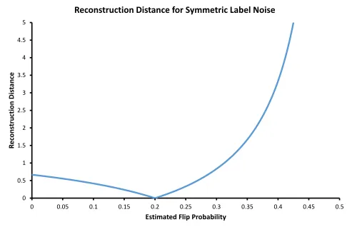
Finally, when working with symmetric label noise (σ−1 =σ1 =σ), kRσ−Rσ0k
1 =
2|σ−σ0| |1−2σ||1−2σ0|.
For fixed true noise rateσ, the presence of a factor|1−2σ0|in the denominator means that underesti-matingσis preferred to overestimating. Hence when designing estimates forσ, those with negative bias might perform better than those that are unbiased or are positively biased. Furthermore, when covering noise rates, as per the discussion in 10, more focus should be given to higher noise rates than to lower.
0 0.5 1 1.5 2 2.5 3 3.5 4 4.5 5
0 0.05 0.1 0.15 0.2 0.25 0.3 0.35 0.4 0.45 0.5
R
ec
o
n
stru
ctio
n
Di
st
ance
Estimated Flip Probability
Reconstruction Distance for Symmetric Label Noise
Figure 1: Plot of kRσ−Rσ0k
1 for σ = 0.2. kRσ−Rσ0k
1 is a measure of how far apart two
corruptions are. This distance measure can be used when constructing estimators for the corruption processT. See text.
A.2 Semi-Supervised Learning
Symmetric Semi-Supervised Learning T σ 0 0 σ
1−σ 1−σ
R∗
1−2σ+2σ2
1−3σ+5σ2−3σ3
−σ2
1−3σ+5σ2−3σ3
−σ2
1−3σ+5σ2−3σ3 1
−2σ+2σ2
1−3σ+5σ2−3σ3
σ
1−2σ+3σ2
σ
1−2σ+3σ2
Clarity(T) σ
kR∗k∞ σ1
k`01,Tk∞ 1−2σ+2σ
2
2σ+3σ−5σ2
Once again k`01,Tk∞ ≤ Clarity(1 T). Our lower bound confirms that in general unlabelled data does not help (Balcan and Blum, 2010). Rather than using the method of unbiased estimators, one could simply throw away the unlabelled data leaving behindσnlabelled instances on average. To make further progress in this problem, as noted elsewhere (Balcan and Blum, 2010), normally one assumes some form of compatibility between the marginal distribution of instances and the optimal classifier. In principle, restricted versions of Le Cams method and the strong data processing inequality could be used to give lower bounds under these different assumptions. As our interest here are minimax bounds, we do not pursue these methods.
A.3 Three Class Symmetric Label Noise
Here we present parameters for the three class variant of symmetric label noise. We haveY˜ =Y = {1,2,3}withP( ˜Y = ˜y|Y =y) = 1−σ, ify= ˜yand σ2 otherwise.
Learning with Symmetric Label Noisy (Multiclass)
T
1−σ σ2 σ2 σ
2 1−σ
σ
2
σ
2
σ
2 1−σ
R∗ 2−σ
2−3σ −σ
2−3σ −σ
2−3σ −σ
2−3σ
2−σ
2−3σ −σ
2−3σ −σ
2−3σ −σ
2−3σ
2−σ
2−3σ
Clarity(T) |1− 32σ| kR∗k∞ |22+−3σσ|
k`01,Tk∞ |2−23σ|max(σ,1−σ)
We see that as long asσ6= 23,T is reconstructible. Once againk`01,Tk∞≤ α(1T).
A.4 Partial Labels
partial label always includes the true label as one of the possibilities and furthermore that spurious labels are added with probabilityσ.
Learning with Partial Labels
T
(1−σ)2 0 0
0 (1−σ)2 0
0 0 (1−σ)2
(1−σ)σ (1−σ)σ 0 (1−σ)σ 0 (1−σ)σ
0 (1−σ)σ (1−σ)σ
σ2 σ2 σ2
R
1 0 0 33−−23σσ 33−−32σσ −3(σ−σ−31) 13 0 1 0 33−−23σσ −3(σ−σ−31) 33−−23σσ 13 0 0 1 −3(σ−σ−31) 33−−32σσ 33−−23σσ 13
Clarity(T) 1−σ
kR∗k∞ |3−σ|3|+21−σ||3−2σ|
k`01,Tk∞ 63−−43σσ
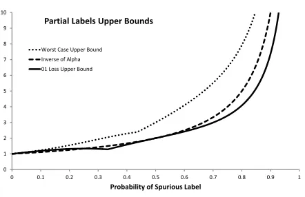
We see that as long asσ 6= 1,T is reconstructible. In this casek`01,Tk∞andkR∗k∞are given by more complicated expressions (however they are both available in closed form). We display their interrelation in a graph in below. To the best of our knowledge, no upper and lower bounds are present in the literature for this problem.
0 1 2 3 4 5 6 7 8 9 10
0 0.1 0.2 0.3 0.4 0.5 0.6 0.7 0.8 0.9 1
Probability of Spurious Label
Partial Labels Upper Bounds
Worst Case Upper Bound
Inverse of Alpha 01 Loss Upper Bound
Appendix B. Le Cam’s Method and Minimax Lower Bounds
The development here closely follows Duchi et al. (2013) with some streamlining. We consider a general decision problem with unknownsΘ, observation spaceZ and lossL : Θ×A → R, with
infaL(θ, a) = 0. For any learning algorithmA ∈ T(Z, A)we wish to lower bound the minimax risk,
RiskL(e) = inf
A supθ Ez∼e(θ)L(θ,A(z)).
The method proceeds by reducing a general decision problem to an easier binary classification problem, by considering a supremum of the risk over a restricted set {θ1, θ2}. Using Markov’s
inequality we then relate this to the minimum01loss in a particular binary classification problem. Finally one finds a lower bound for this quantity. Withθ∼{θ1, θ2}meaningθis drawn uniformly at
random from the set{θ1, θ2}, we have, sup
θ
Ez∼e(θ)Ea∼A(z)L(θ, a)≥ sup
{θ1,θ2}
Ez∼e(θ)Ea∼A(z)L(θ, a) ≥Eθ∼{θ1,θ2}Ez∼e(θ)Ea∼A(z)L(θ, a)
≥δEθ∼{θ1,θ2}Ez∼e(θ)Ea∼A(z)[[L(θ, a)≥δ]].
Recall theseparationρ: Θ×Θ→R,ρ(θ1, θ2) = infaL(θ1, a)+L(θ2, a). The separation measures
how hard it is to act well against bothθ1 andθ2 simultaneously. We now assumeρ(θ1, θ2) > 2δ.
Definef :A→ {θ1, θ2,error}wheref(a) =θi ifL(θi, a)< δand error otherwise. This function is well defined as if there exists an actionawithL(θ1, a)< δandL(θ2, a)< δthenρ(θ1, θ2)<2δ,
a contradiction. LetAˆbe the classifier that first drawsa∼A(z)and then outputsf(a). We have,
sup
θ
Ez∼e(θ)Ea∼A(z)L(θ, a)≥δEθ∼{θ1,θ2}Ez∼e(θ)Eθ0∼Aˆ(z)[[θ6=θ0]] ≥δ inf
ˆ
A∈T(Z,Θ)
Eθ∼{θ1,θ2}Ez∼e(θ)Eθ0∼Aˆ(z)[[θ6=θ0]]
=δ
1 2 −
1
2V(e(θ1), e(θ2))
,
where the first line is a rewriting of of the previous in terms of the classifierAˆ, the second takes an infimum over all classifiers and the final line is a standard result in theoretical statistics (see Reid and Williamson (2011) for a modern treatment). Takingδ = ρ(θ1,θ2)
2 yields lemma 8. B.1 Extension of Le Cam’s Method to Bayesian Risk
Rather than lower boundingsupθEz∼e(θ)L(θ,A(z)), a Bayesian with some knowledge about the
unknown, given in the form of a priorπ ∈P(Θ), wishes to lower bound the Bayesian risk,
RiskπL(e) := inf
A Eθ∼πEz∼e(θ)L(θ,A(z)).
Following from the second line of the derivation of Le Cam’s method, we have a lower bound,
Eθ∼{θ1,θ2}Ez∼e(θ)Ea∼A(z)L(θ, a) = 1
2RiskL(θ1, e,A) + 1
2RiskL(θ2, e,A) ≥ρ(θ1, θ2)
1 4 −
1
4V(e(θ1), e(θ2))
Letµ∈P(Θ×Θ)be any distribution withbothmarginals overΘequal toπ. Averaging over this distribution we have,
Eθ∼πRiskL(θ, e,A)≥E(θ1,θ2)∼µρ(θ1, θ2)
1 4−
1
4V(e(θ1), e(θ2))
.
This insight leads to a Bayesian version of lemma 8.
Lemma 36 Letµ∈P(Θ×Θ)be any distribution withbothmarginals overΘequal toπ. Then for
all experimentseand loss functions`,
RiskπL(e)≥E(θ1,θ2)∼µρ(θ1, θ2)
1 4−
1
4V(e(θ1), e(θ2))
.
Using this in place of lemma 8 leads to Bayesian versions of theorems 15 and 16.
Appendix C. Canonical Loss Functions and their Convexification
Here we developgeneralrepresentations of loss functionsL: Θ×A→R. We assume that the set
Θis finite.
In many statistical problems, it is natural for the space of actionsA to be the set of distributions over unknownsP(Θ).
Definition 37 A lossL: Θ×P(Θ)→Risproperif for all distributionsP ∈P(Θ),
P ∈arg min
Q∈P(Θ)
hP, L(−, Q)iΘ.
It isstrictly properifPis theuniqueminimizer.
A proper loss takes a predictionQ∈P(Θ), and then penalizes the decision maker according to how much weight their prediction assigned to the unknownθ. Intuitively properness ensures that if the decision makerknowsP, then they minimize their expected loss byreportingP. Proper losses con-stitute a well studied class of loss functions, that provide suitable surrogates for decision problems (Brier, 1950; Gr¨unwald and Dawid, 2004; Zhang, 2004; Gneiting and Raftery, 2007; Dawid, 2007; Reid and Williamson, 2009a; Dawid, 2007; ´Avila Pires et al., 2013).
As will be shown, all “sensible” losses are essentially re-parametrized proper losses. We show how
toconstructproper losses from their entropies. Furthermore, we show how to render any proper loss
convex through a canonical re-parametrization. This allows the use of tools from convex analysis (Boyd and Vandenberghe, 2004; Lucchetti, 2006) to aid in calculating optimal actions.
C.1 Entropy from Loss
Rather than working with probability distributions, we take the route of Williamson (2014) and work with un-normalized distributions. Denote the set of all unnormalized distributions on Θby
P+(Θ). For any loss functionL, define theentropyL:P+(Θ)→R, L(µ) = min
L(P) measures the uncertainty of the optimal action for the distribution P. The entropy is also called an uncertainty function, a Bayes risk or a support function (DeGroot, 1962; Williamson, 2014). It is concave and 1-homogeneous.
Definition 38 A functionf :P+(Θ)→Ris 1-homogeneous if for allx∈P+(Θ)and for allλ >0,
f(λx) =λf(x).
C.2 Loss from Entropy
All loss functions give rise to an entropy. Conversely, the entropy encodes much information of its associated loss through itssuper-gradients, which include all theBayesactions for the underlying loss.
C.2.1 BAYESACTIONS ANDSUPER-GRADIENTS
For any distributionP, define theBayes actionsforP as the set of minimizers,
AP = arg min a∈A
hP, L(−, a)i.
For anyaP ∈AP we haveL(P) =hP, L(−, aP)i.
Definition 39 (Super-gradient of a concave function) Letf :P+(Θ)→Rbe a concave function.
v∈RΘis asuper-gradientoff at the pointxif for ally∈P+(Θ),
hy−x, vi+f(x)≥f(y).
Denote the set of all super-gradients at a pointx by ∂f(x), and the set of all super-gradients by ∂f = ∪x∂f(x). For differentiable concave functions, super-gradients are the same as regular gradients (Lucchetti, 2006). 1-homogeneous functions afford a very simple representation via their super-gradients.
Theorem 40 (Generalized Euler’s Homogeneous Function Theorem) Let
f :P+(Θ)→Rbe a concave 1-homogeneous function. Then for allxand for allv∈∂f(x),
f(x) =hx, vi.
Furthermore,v∈∂f(x) =⇒ v ∈∂f(λx)for allλ >0.
We include a simple proof of this theorem for completeness.
Proof Firstly, for allxand allλ >0,
hλx−x, vi+f(x)≥λf(x),
which follows directly from the definition of a super-gradient at x and the 1-homogeneity of f. Re-arranging yields,(1−λ)(f(x)− hx, vi)≥0. Lettingλ→0+yieldsf(x)≥ hx, vi. Similarly, for allxand allλ >0,