Catalyst Acceleration for First-order Convex Optimization:
from Theory to Practice
Hongzhou Lin [email protected]
Massachusetts Institute of Technology
Computer Science and Artificial Intelligence Laboratory Cambridge, MA 02139, USA
Julien Mairal [email protected]
Univ. Grenoble Alpes, Inria, CNRS, Grenoble INP∗, LJK, Grenoble, 38000, France
Zaid Harchaoui [email protected]
University of Washington Department of Statistics Seattle, WA 98195, USA
Editor:L´eon Bottou
Abstract
We introduce a generic scheme for accelerating gradient-based optimization methods in the sense of Nesterov. The approach, called Catalyst, builds upon the inexact acceler-ated proximal point algorithm for minimizing a convex objective function, and consists of approximately solving a sequence of well-chosen auxiliary problems, leading to faster con-vergence. One of the keys to achieve acceleration in theory and in practice is to solve these sub-problems with appropriate accuracy by using the right stopping criterion and the right warm-start strategy. We give practical guidelines to use Catalyst and present a compre-hensive analysis of its global complexity. We show that Catalyst applies to a large class of algorithms, including gradient descent, block coordinate descent, incremental algorithms such as SAG, SAGA, SDCA, SVRG, MISO/Finito, and their proximal variants. For all of these methods, we establish faster rates using the Catalyst acceleration, for strongly convex and non-strongly convex objectives. We conclude with extensive experiments showing that acceleration is useful in practice, especially for ill-conditioned problems.
Keywords: convex optimization, first-order methods, large-scale machine learning
1. Introduction
A large number of machine learning and signal processing problems are formulated as the minimization of a convex objective function:
min
x∈Rp
n
f(x),f0(x) +ψ(x)
o
, (1)
where f0 is convex and L-smooth, andψ is convex but may not be differentiable. We call a function L-smooth when it is differentiable and its gradient isL-Lipschitz continuous.
∗. Institute of Engineering Univ. Grenoble Alpes
c
In statistics or machine learning, the variable x may represent model parameters, and the role off0is to ensure that the estimated parameters fit some observed data. Specifically,
f0 is often a large sum of functions and (1) is a regularized empirical risk which writes as
min
x∈Rp
(
f(x), 1
n
n
X
i=1
fi(x) +ψ(x)
)
. (2)
Each term fi(x) measures the fit between x and a data point indexed by i, whereas the
function ψ acts as a regularizer; it is typically chosen to be the squared `2-norm, which is smooth, or to be a non-differentiable penalty such as the `1-norm or another sparsity-inducing norm (Bach et al., 2012).
We present a unified framework allowing one to accelerate gradient-based or first-order methods, with a particular focus on problems involving large sums of functions. By “ac-celerating”, we mean generalizing a mechanism invented by Nesterov (1983) that improves the convergence rate of the gradient descent algorithm. When ψ = 0, gradient descent steps produce iterates (xk)k≥0 such that f(xk)−f∗ ≤ ε in O(1/ε) iterations, where f∗
denotes the minimum value off. Furthermore, when the objective f is µ-strongly convex, the previous iteration-complexity becomes O((L/µ) log(1/ε)), which is proportional to the condition number L/µ. However, these rates were shown to be suboptimal for the class of first-order methods, and a simple strategy of taking the gradient step at a well-chosen point different from xk yields the optimal complexity—O(1/
√
ε) for the convex case and
O(pL/µlog(1/ε)) for the µ-strongly convex one (Nesterov, 1983). Later, this acceleration technique was extended to deal with non-differentiable penaltiesψ for which the proximal operator defined below is easy to compute (Beck and Teboulle, 2009; Nesterov, 2013).
proxψ(x),arg min
z∈Rp
ψ(z) +1
2kx−zk 2
, (3)
wherek.k denotes the Euclidean norm.
For machine learning problems involving a large sum ofn functions, a recent effort has been devoted to developing fast incremental algorithms such as SAG (Schmidt et al., 2017), SAGA (Defazio et al., 2014a), SDCA (Shalev-Shwartz and Zhang, 2012), SVRG (Johnson and Zhang, 2013; Xiao and Zhang, 2014), or MISO/Finito (Mairal, 2015; Defazio et al., 2014b), which can exploit the particular structure (2). Unlike full gradient approaches, which require computing and averaging n gradients (1/n)Pn
i=1∇fi(x) at every iteration, incremental techniques have a cost per-iteration that is independent ofn. The price to pay is the need to store a moderate amount of information regarding past iterates, but the benefits may be significant in terms of computational complexity. In order to achieve anε-accurate solution for a µ-strongly convex objective, the number of gradient evaluations required by the methods mentioned above is bounded by O
n+Lµ¯
log(1ε)
, where ¯L is either the maximum Lipschitz constant across the gradients ∇fi, or the average value, depending
on the algorithm variant considered. Unless there is a big mismatch between ¯L and L
(global Lipschitz constant for the sum of gradients), incremental approaches significantly outperform the full gradient method, whose complexity in terms of gradient evaluations is bounded by O
nLµlog(1ε)
Yet, these incremental approaches do not use Nesterov’s extrapolation steps and whether or not they could be accelerated was an important open question when these methods were introduced. It was indeed only known to be the case for SDCA (Shalev-Shwartz and Zhang, 2016) for strongly convex objectives. Later, other accelerated incremental algorithms were proposed such as Katyusha (Allen-Zhu, 2017), or the method of Lan and Zhou (2017).
We give here a positive answer to this open question. By analogy with substances that increase chemical reaction rates, we call our approach “Catalyst”. Given an optimization methodMas input, Catalyst outputs an accelerated version of it, eventually the same algo-rithm if the methodMis already optimal. The sole requirement on the method in order to achieve acceleration is that it should have linear convergence rate for strongly convex prob-lems. This is the case for full gradient methods (Beck and Teboulle, 2009; Nesterov, 2013) and block coordinate descent methods (Nesterov, 2012; Richt´arik and Tak´aˇc, 2014), which already have well-known accelerated variants. More importantly, it also applies to the pre-viou incremental methods, whose complexity is then bounded by ˜On+pnL/µ¯ log(1ε) after Catalyst acceleration, where ˜O hides some logarithmic dependencies on the condition number ¯L/µ. This improves upon the non-accelerated variants, when the condition num-ber is larger thann. Besides, acceleration occurs regardless of the strong convexity of the objective—that is, even ifµ= 0—which brings us to our second achievement.
Some approaches such as MISO, SDCA, or SVRG are only defined for strongly convex objectives. A classical trick to apply them to general convex functions is to add a small regularization termεkxk2in the objective (Shalev-Shwartz and Zhang, 2012). The drawback of this strategy is that it requires choosing in advance the parameter ε, which is related to the target accuracy. The approach we present here provides a direct support for
non-strongly convex objectives, thus removing the need of selecting εbeforehand. Moreover, we
can immediately establish a faster rate for the resulting algorithm. Finally, some methods such as MISO are numerically unstable when they are applied to strongly convex objective functions with small strong convexity constant. By defining better conditioned auxiliary subproblems, Catalyst also provides better numerical stability to these methods.
A short version of this paper has been published at the NIPS conference in 2015 (Lin et al., 2015a); in addition to simpler convergence proofs and more extensive numerical evalu-ation, we extend the conference paper with a new Moreau-Yosida smoothing interpretation with significant theoretical and practical consequences as well as new practical stopping criteria and warm-start strategies.
The paper is structured as follows. We complete this introductory section with some related work in Section 1.1, and give a short description of the two-loop Catalyst algorithm in Section 1.2. Then, Section 2 introduces the Moreau-Yosida smoothing and its inexact variant. In Section 3, we introduce formally the main algorithm, and its convergence analysis is presented in Section 4. Section 5 is devoted to numerical experiments and Section 6 concludes the paper.
1.1 Related Work
Boyd, 2014). The proximal point algorithm consists of solving (1) by minimizing a sequence of auxiliary problems involving a quadratic regularization term. In general, these auxiliary problems cannot be solved with perfect accuracy, and several notions of inexactness were proposed by G¨uler (1992); He and Yuan (2012) and Salzo and Villa (2012). The Cata-lyst approach hinges upon (i) an acceleration technique for the proximal point algorithm originally introduced in the pioneer work of G¨uler (1992); (ii) a more practical inexact-ness criterion than those proposed in the past.1 As a result, we are able to control the rate of convergence for approximately solving the auxiliary problems with an optimization methodM. In turn, we are also able to obtain the computational complexity of the global procedure, which was not possible with previous analysis (G¨uler, 1992; He and Yuan, 2012; Salzo and Villa, 2012). When instantiated in different first-order optimization settings, our analysis yields systematic acceleration.
Beyond G¨uler (1992), several works have inspired this work. In particular, accelerated SDCA (Shalev-Shwartz and Zhang, 2016) is an instance of an inexact accelerated proximal point algorithm, even though this was not explicitly stated in the original paper. Catalyst can be seen as a generalization of their algorithm, originally designed for stochastic dual coordinate ascent approaches. Yet their proof of convergence relies on different tools than ours. Specifically, we introduce an approximate sufficient descent condition, which, when satisfied, grants acceleration to any optimization method, whereas the direct proof of Shalev-Shwartz and Zhang (2016), in the context of SDCA, does not extend to non-strongly convex objectives. Another useful methodological contribution was the convergence analysis of inexact proximal gradient methods of Schmidt et al. (2011) and Devolder et al. (2014). Finally, similar ideas appeared in the independent work (Frostig et al., 2015). Their results partially overlap with ours, but the two papers adopt rather different directions. Our analysis is more general, covering both strongly-convex and non-strongly convex objectives, and comprises several variants including an almost parameter-free variant.
Then, beyond accelerated SDCA (Shalev-Shwartz and Zhang, 2016), other accelerated incremental methods have been proposed, such as APCG (Lin et al., 2015b), SDPC (Zhang and Xiao, 2015), RPDG (Lan and Zhou, 2017), Point-SAGA (Defazio, 2016) and Katyusha (Allen-Zhu, 2017). Their techniques are algorithm-specific and cannot be directly general-ized into a unified scheme. However, we should mention that the complexity obtained by applying Catalyst acceleration to incremental methods matches the optimal bound up to a logarithmic factor, which may be the price to pay for a generic acceleration scheme.
A related recent line of work has also combined smoothing techniques with outer-loop algorithms such as Quasi-Newton methods (Themelis et al., 2016; Giselsson and F¨alt, 2016). Their purpose was not to accelerate existing techniques, but rather to derive new algorithms for nonsmooth optimization.
To conclude this survey, we mention the broad family of extrapolation methods (Sidi, 2017), which allow one to extrapolate to the limit sequences generated by iterative al-gorithms for various numerical analysis problems. Scieur et al. (2016) proposed such an approach for convex optimization problems with smooth and strongly convex objectives. The approach we present here allows us to obtain global complexity bounds for strongly
Algorithm 1 Catalyst - Overview
input initial estimate x0 inRp, smoothing parameter κ, optimization methodM.
1: Initialize y0=x0.
2: whilethe desired accuracy is not achieveddo
3: Find xk usingM
xk ≈arg min
x∈Rp
n
hk(x),f(x) +
κ
2kx−yk−1k
2o. (4)
4: Compute yk using an extrapolation step, withβk in (0,1)
yk=xk+βk(xk−xk−1).
5: end while
output xk (final estimate).
convex and non strongly convex objectives, which can be decomposed into a smooth part and a non-smooth proximal-friendly part.
1.2 Overview of Catalyst
Before introducing Catalyst precisely in Section 3, we give a quick overview of the algo-rithm and its main ideas. Catalyst is a generic approach that wraps an algoalgo-rithm Minto an accelerated one A, in order to achieve the same accuracy asMwith reduced computa-tional complexity. The resulting method A is an inner-outer loop construct, presented in Algorithm 1, where in theinner loop the methodMis called to solve an auxiliary strongly-convex optimization problem, and where in theouter loop the sequence of iterates produced
by M are extrapolated for faster convergence. There are therefore three main ingredients
in Catalyst: a) a smoothing technique that produces strongly-convex sub-problems; b) an extrapolation technique to accelerate the convergence; c) a balancing principle to optimally tune the inner and outer computations.
Smoothing by infimal convolution Catalyst can be used on any algorithm M that enjoys a linear-convergence guarantee when minimizing strongly-convex objectives. How-ever the objective at hand may be poorly conditioned or even might not be strongly convex. In Catalyst, we useMtoapproximately minimize an auxiliary objective hk at iterationk,
defined in (4), which is strongly convex and better conditioned than f. Smoothing by infimal convolution allows one to build a well-conditioned convex functionF from a poorly-conditioned convex function f (see Section 3 for a refresher on Moreau envelopes). We shall show in Section 3 that a notion of approximate Moreau envelope allows us to define precisely the information collected when approximately minimizing the auxiliary objective.
Extrapolation by Nesterov acceleration Catalyst uses an extrapolation scheme “ `a la Nesterov ” to build a sequence (yk)k≥0 updated as
yk=xk+βk(xk−xk−1),
Without Catalyst With Catalyst
µ >0 µ= 0 µ >0 µ= 0
FG OnLµlog 1ε
O nLε ˜
OnqLµlog 1ε ˜
O
n
q
L ε
SAG/SAGA
O
n+Lµ¯
log 1ε
O
nL¯ε
˜
On+
q
nL¯ µ
log 1ε ˜
O
q
nL¯ ε
MISO
not avail. SDCA
SVRG
Acc-FG O
nqLµlog 1ε
O
n√L ε
no acceleration Acc-SDCA O˜
n+
q
nL¯ µ
log 1ε
not avail.
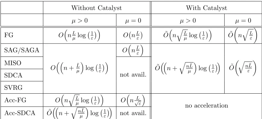
Table 1: Comparison of rates of convergence, before and after the Catalyst acceleration, in the strongly-convex and non strongly-convex cases, respectively. The notation ˜O
hides logarithmic factors. The constantL is the global Lipschitz constant of the gradient’s objective, while ¯L is the average Lipschitz constants of the gradients
∇fi, or the maximum value, depending on the algorithm’s variants considered.
We shall show in Section 4 that we can get faster rates of convergence thanks to this extrapolation step when the smoothing parameterκ, the inner-loop stopping criterion, and the sequence (βk)k≥0 are carefully built.
Balancing inner and outer complexities The optimal balance between inner loop and outer loop complexity derives from the complexity bounds established in Section 4. Given an estimate about the condition number off, our bounds dictate a choice ofκthat gives the optimal setting for the inner-loop stopping criterion and all technical quantities involved in the algorithm. We shall demonstrate in particular the power of an appropriate warm-start strategy to achieve near-optimal complexity.
Overview of the complexity results Finally, we provide in Table 1 a brief overview of the complexity results obtained from the Catalyst acceleration, when applied to various optimization methods M for minimizing a large finite sum of n functions. Note that the complexity results obtained with Catalyst are optimal, up to some logarithmic factors (see Agarwal and Bottou, 2015; Arjevani and Shamir, 2016; Woodworth and Srebro, 2016).
2. The Moreau Envelope and its Approximate Variant
which can turn any convex lower semicontinuous functionf into a smooth function, and an ill-conditioned smooth convex function into a well-conditioned smooth convex function.
The Moreau envelope results from the infimal convolution off with a quadratic penalty:
F(x),min
z∈Rp
n
f(z) +κ
2kz−xk
2o, (5)
where κ is a positive regularization parameter. The proximal operator is then the unique minimizer of the problem—that is,
p(x),proxf /κ(x) = arg min
z∈Rp
n
f(z) +κ
2kz−xk 2o.
Note that p(x) does not admit a closed form in general. Therefore, computing it requires to solve the sub-problem to high accuracy with some iterative algorithm.
2.1 Basic Properties of the Moreau Envelope
The smoothing effect of the Moreau regularization can be characterized by the next propo-sition (see Lemar´echal and Sagastiz´abal, 1997, for elementary proofs).
Proposition 1 (Regularization properties of the Moreau Envelope) Given a
con-vex continuous function f and a regularization parameter κ > 0, consider the Moreau
envelope F defined in (5). Then,
1. F is convex and minimizingf andF are equivalent in the sense that
min
x∈RpF(x) = minx∈
Rp
f(x).
Moreover the solution set of the two above problems coincide with each other.
2. F is continuously differentiable even when f is not and
∇F(x) =κ(x−p(x)). (6)
Moreover the gradient∇F is Lipschitz continuous with constant LF =κ.
3. If f isµ-strongly convex, then F is µF-strongly convex withµF = µµκ+κ.
Interestingly,F is friendly from an optimization point of view as it is convex and differen-tiable. Besides, F is κ-smooth with condition number µ+µκ when f is µ-strongly convex. ThusF can be made arbitrarily well conditioned by choosing a smallκ. Since both functions
f and F admit the same solutions, a naive approach to minimize a non-smooth functionf
is to first construct its Moreau envelope F and then apply a smooth optimization method on it. As we will see next, Catalyst can be seen as an accelerated gradient descent technique applied toF with inexact gradients.
2.2 A Fresh Look at Catalyst
The proximal point algorithm. Consider gradient descent steps onF:
xk+1 =xk−
1
LF
∇F(xk).
By noticing that ∇F(xk) =κ(xk−p(xk)) andLf =κ, we obtain in fact
xk+1 =p(xk) = arg min
z∈Rp
n
f(z) +κ
2kz−xkk 2o,
which is exactly the proximal point algorithm (Martinet, 1970; Rockafellar, 1976).
Accelerated proximal point algorithm. If gradient descent steps on F yields the proximal point algorithm, it is then natural to consider the following sequence
xk+1=yk−
1
LF
∇F(yk) and yk+1=xk+1+βk+1(xk+1−xk),
where βk+1 is Nesterov’s extrapolation parameter (Nesterov, 2004). Again, by using the closed form of the gradient, this is equivalent to the update
xk+1=p(yk) and yk+1=xk+1+βk+1(xk+1−xk),
which is known as the accelerated proximal point algorithm of G¨uler (1992).
While these algorithms are conceptually elegant, they suffer from a major drawback in practice: each update requires to evaluate the proximal operator p(x). Unless a closed form is available, which is almost never the case, we are not able to evaluate p(x) exactly. Hence an iterative algorithm is required for each evaluation of the proximal operator which leads to the inner-outer construction (see Algorithm 1). Catalyst can then be interpreted as an accelerated proximal point algorithm that calls an optimization methodMto compute inexact solutions to the sub-problems. The fact that such a strategy could be used to solve non-smooth optimization problems was well-known, but the fact that it could be used for acceleration is more surprising. The main challenge that will be addressed in Section 3 is how to control the complexity of the inner-loop minimization.
2.3 The Approximate Moreau Envelope
Since Catalyst uses inexact gradients of the Moreau envelope, we start with specifying the inexactness criteria.
Inexactness through absolute accuracy. Given a proximal center x, a smoothing parameterκ, and an accuracyε >0, we denote the set of ε-approximations of the proximal operatorp(x) by
pε(x),{z∈Rp s.t. h(z)−h∗ ≤ε} where h(z) =f(z) +κ
2kx−zk
2, (C1) and h∗ is the minimum function value of h.
d(z) ≤h∗, we can guarantee z ∈pε(x) if h(z)−d(z) ≤ε. There are other choices for the lower bounding function d which result from the specific construction of the optimization algorithm. For instance, dual type algorithms such as SDCA (Shalev-Shwartz and Zhang, 2012) or MISO (Mairal, 2015) maintain a lower bound along the iterations, allowing one to computeh(z)−d(z)≤ε.
When none of the options mentioned above are available, we can use the following fact, based on the notion of gradient mapping; see Section 2.3.2 of (Nesterov, 2004). The intuition comes from the smooth case: when h is smooth, the strong convexity yields
h(z)− 1
2κk∇h(z)k
2 ≤h∗
.
In other words, the norm of the gradient provides enough information to assess how far we are from the optimum. From this perspective, the gradient mapping can be seen as an extension of the gradient for the composite case where the objective decomposes as a sum of a smooth part and a non-smooth part (Nesterov, 2004).
Lemma 2 (Checking the absolute accuracy criterion) Consider a proximal centerx,
a smoothing parameter κ and an accuracyε >0. Consider an objective with the composite
form (1) and we set function h as
h(z) =f(z) + κ
2kx−zk 2=f
0(z) +
κ
2kx−zk 2
| {z }
,h0
+ψ(x).
For any z∈Rp, we define
[z]η = proxηψ(z−η∇h0(z)), with η= 1
κ+L. (7)
Then, the gradient mapping of h atz is defined by 1η(z−[z]η) and
1
ηkz−[z]ηk ≤
√
2κε implies [z]η ∈pε(x).
The proof is given in Appendix B. The lemma shows that it is sufficient to check the norm of the gradient mapping to ensure condition (C1). However, this requires an additional full gradient step and proximal step at each iteration.
As soon as we have an approximate proximal operator zinpε(x) in hand, we can define an approximate gradient of the Moreau envelope,
g(z),κ(x−z), (8)
by mimicking the exact gradient formula∇F(x) =κ(x−p(x)). As a consequence, we may immediately draw a link
z∈pε(x) =⇒ kz−p(x)k ≤
r 2ε
κ ⇐⇒ kg(z)− ∇F(x)k ≤
√
2κε, (9)
Relative error criterion. Another natural way to bound the gradient approximation is by using a relative error, namely in the formkg(z)− ∇F(x)k ≤δ0k∇F(x)kfor someδ0 >0. This leads us to the following inexactness criterion.
Given a proximal centerx, a smoothing parameterκ and a relative accuracyδ in [0,1), we denote the set ofδ-relative approximations by
gδ(x),
z∈Rp s.t. h(z)−h∗≤ δκ
2 kx−zk 2
, (C2)
At a first glance, we may interpret the criterion (C2) as (C1) by setting ε = δκ2 kx−zk2. But we should then notice that the accuracy depends on the pointz, which is is no longer an absolute constant. In other words, the accuracy varies from point to point, which is proportional to the squared distance betweenzandx. First one may wonder whethergδ(x) is an empty set. Indeed, it is easy to see that p(x) ∈ gδ(x) since h(p(x))−h∗ = 0 ≤
δκ
2 kx−p(x)k2. Moreover, by continuity,gδ(x) is closed set aroundp(x). Then, by following similar steps as in (9), we have
z∈gδ(x) =⇒ kz−p(x)k ≤√δkx−zk ≤√δ(kx−p(x)k+kp(x)−zk).
By defining the approximate gradient in the same way g(z) =κ(x−z) yields,
z∈gδ(x) =⇒ kg(z)− ∇F(x)k ≤δ0k∇F(x)k with δ0 =
√
δ
1−√δ,
which is the desired relative gradient approximation.
Finally, the discussion about boundingh(z)−h∗ still holds here. In particular, Lemma 2 may be used by setting the valueε= δκ2kx−zk2. The price to pay is as an additional gradient step and an additional proximal step per iteration.
A few remarks on related works. Inexactness criteria with respect to subgradient norms have been investigated in the past, starting from the pioneer work of Rockafel-lar (1976) in the context of the inexact proximal point algorithm. Later, different works have been dedicated to more practical inexactness criteria (Auslender, 1987; Correa and Lemar´echal, 1993; Solodov and Svaiter, 2001; Fuentes et al., 2012). These criteria include duality gap, ε-subdifferential, or decrease in terms of function value. Here, we present a more intuitive point of view using the Moreau envelope.
While the proximal point algorithm has caught a lot of attention, very few works have focused on its accelerated variant. The first accelerated proximal point algorithm with inexact gradients was proposed by G¨uler (1992). Then, Salzo and Villa (2012) proposed a more rigorous convergence analysis, and more inexactness criteria, which are typically stronger than ours. In the same way, a more general inexact oracle framework has been proposed later by Devolder et al. (2014). To achieve the Catalyst acceleration, our main effort was to propose and analyze criteria that allow us to control the complexity for finding approximate solutions of the sub-problems.
3. Catalyst Acceleration
gradient descent method applied to the Moreau envelope of the objective with inexact gradi-ents. Since an overview has already been presented in Section 1.2, we now present important details to obtain acceleration in theory and in practice.
Algorithm 2 Catalyst
input Initial estimate x0 in Rp, smoothing parameter κ, strong convexity parameter µ,
optimization method M and a stopping criterion based on a sequence of accuracies (εk)k≥0, or (δk)k≥0, or a fixed budget T.
1: Initialize y0=x0,q= µ+µκ. Ifµ >0, set α0 =
√
q, otherwiseα0 = 1.
2: whilethe desired accuracy is not achieveddo
3: Compute an approximate solution of the following problem withM
xk ≈arg min
x∈Rp
n
hk(x),f(x) +
κ
2kx−yk−1k 2o,
using the warm-start strategy of Section 3 and one of the following stopping criteria:
(a) absolute accuracy: find xk inpεk(yk−1) by using criterion (C1);
(b) relative accuracy: find xk ingδk(yk−1) by using criterion (C2);
(c) fixed budget: runMforT iterations and outputxk.
4: Updateαk in (0,1) by solving the equation
α2k= (1−αk)α2k−1+qαk. (10)
5: Compute yk with Nesterov’s extrapolation step
yk =xk+βk(xk−xk−1) with βk=
αk−1(1−αk−1)
α2k−1+αk
. (11)
6: end while
output xk (final estimate).
Requirement: linear convergence of the methodM. One of the main characteristic of Catalyst is to apply the method Mto strongly-convex sub-problems, without requiring strong convexity of the objective f. As a consequence, Catalyst provides direct support for convex but non-strongly convex objectives to M, which may be useful to extend the scope of application of techniques that need strong convexity to operate. Yet, Catalyst requires solving these sub-problems efficiently enough in order to control the complexity of the inner-loop computations. When applyingMto minimize a strongly-convex functionh, we assume thatMis able to produce a sequence of iterates (zt)t≥0 such that
h(zt)−h∗ ≤CM(1−τM)t(h(z0)−h∗), (12)
wherez0 is the initial point given toM, andτMin (0,1),CM>0 are two constants. In such
of convergence for solving the sub-problems: the larger isτM, the faster is the convergence.
For a given algorithm M, the quantity τM depends usually on the condition number of h.
For instance, for the proximal gradient method and many first-order algorithms, we simply haveτM=O((µ+κ)/(L+κ)), ashis (µ+κ)-strongly convex and (L+κ)-smooth. Catalyst
can also be applied to randomized methods Mthat satisfy (12) in expectation:
E[h(zt)−h∗]≤CM(1−τM)t(h(z0)−h∗), (13)
Then, the complexity results of Section 4 also hold in expectation. This allows us to apply Catalyst to randomized block coordinate descent algorithms (see Richt´arik and Tak´aˇc, 2014, and references therein), and some incremental algorithms such as SAG, SAGA, or SVRG. For other methods that admit a linear convergence rates in terms of duality gap, such as SDCA, MISO/Finito, Catalyst can also be applied as explained in Appendix C.
Stopping criteria. Catalyst may be used with three types of stopping criteria for solving the inner-loop problems. We now detail them below.
(a) absolute accuracy: we predefine a sequence (εk)k≥0 of accuracies, and stop the
method Mby using the absolute stopping criterion (C1). Our analysis suggests
– iff isµ-strongly convex,
εk=
1
2(1−ρ)
k(f(x
0)−f∗) with ρ <
√
q .
– iff is convex but not strongly convex,
εk=
f(x0)−f∗
2(k+ 2)4+γ with γ >0.
Typically, γ = 0.1 and ρ = 0.9√q are reasonable choices, both in theory and in practice. Of course, the quantity f(x0)−f∗ is unknown and we need to upper bound it by a duality gap or by Lemma 2 as discussed in Section 2.3.
(b) relative accuracy: To use the relative stopping criterion (C2), our analysis suggests
the following choice for the sequence (δk)k≥0: – iff isµ-strongly convex,
δk=
√
q
2−√q .
– iff is convex but not strongly convex,
δk =
1 (k+ 1)2 .
(c) fixed budget: Finally, the simplest way of using Catalyst is to fix in advance the
checking any optimality criterion. Whereas our analysis provides theoretical bud-gets that are compatible with this strategy, we found them to be pessimistic and impractical. Instead, we propose an aggressive strategy for incremental methods that simply consists of setting T = n. This setting was called the “one-pass” strategy in the original Catalyst paper (Lin et al., 2015a).
Warm-starts in inner loops. Besides linear convergence rate, an adequate warm-start strategy needs to be used to guarantee that the sub-problems will be solved in reasonable computational time. The intuition is that the previous solution may still be a good ap-proximation of the current subproblem. Specifically, the following choices arise from the convergence analysis that will be detailed in Section 4.
Consider the minimization of the (k+ 1)-th subproblemhk+1(z) =f(z) + κ2kz−ykk2,
we warm start the optimization methodMatz0 as following: (a) when using criterion (C1) to findxk+1 inpεk(yk),
– iff is smooth (ψ= 0), then choosez0=xk+κ+κµ(yk−yk−1).
– iff is composite as in (1), then definew0 =xk+κ+κµ(yk−yk−1) and
z0 = [w0]η = proxηψ(w0−ηg) with η = 1
L+κ and g=∇f0(w0)+κ(w0−yk).
(b) when using criteria (C2) to find xk+1 ingδk(yk),
– iff is smooth (ψ= 0), then choosez0=yk.
– iff is composite as in (1), then choose
z0= [yk]η = proxηψ(yk−η∇f0(yk)) with η=
1
L+κ.
(c) when using a fixed budget T, choose the same warm start strategy as in (b).
Note that the earlier conference paper (Lin et al., 2015a) considered the the warm start rule z0 =xk−1. That variant is also theoretically validated but it does not perform as well as the ones proposed here in practice.
Optimal balance: choice of parameter κ. Finally, the last ingredient is to find an optimal balance between the inner-loop (for solving each sub-problem) and outer-loop com-putations. To do so, we minimize our global complexity bounds with respect to the value of κ. As we shall see in Section 5, this strategy turns out to be reasonable in practice. Then, as shown in the theoretical section, the resulting rule of thumb is
We select κ by maximizing the ratio τM/ √
We recall that τM characterizes how fast M solves the sub-problems, according to (12);
typically,τM depends on the condition number Lµ++κκ and is a function ofκ.2 In Table 2, we
illustrate the choice ofκ for different methods. Note that the resulting rule for incremental methods is very simple for the pracitioner: select κ such that the condition number Lµ¯++κκ is of the order ofn; then, the inner-complexity becomesO(nlog(1/ε)).
Method M Inner-complexity τM Choice for κ
FG O
nLµ++κκlog 1ε
∝ µL++κκ L−2µ
SAG/SAGA/SVRG On+µL¯++κκlog 1ε
∝ µ+κ
n(µ+κ)+ ¯L+κ
¯
L−µ
n+1 −µ
Table 2: Example of choices of the parameterκ for the full gradient (FG) and incremental methods SAG/SAGA/SVRG. See Table 1 for details about the complexity.
4. Convergence and Complexity Analysis
We now present the complexity analysis of Catalyst. In Section 4.1, we analyze the con-vergence rate of the outer loop, regardless of the complexity for solving the sub-problems. Then, we analyze the complexity of the inner-loop computations for our various stopping criteria and warm-start strategies in Section 4.2. Section 4.3 combines the outer- and inner-loop analysis to provide the global complexity of Catalyst applied to a given optimization method M.
4.1 Complexity Analysis for the Outer-Loop
The complexity analysis of the first variant of Catalyst we presented in (Lin et al., 2015a) used a tool called “estimate sequence”, which was introduced by Nesterov (2004). Here, we provide a simpler proof. We start with criterion (C1), before extending the result to (C2).
4.1.1 Analysis for Criterion (C1)
The next theorem describes how the errors (εk)k≥0 accumulate in Catalyst.
Theorem 3 (Convergence of outer-loop for criterion (C1)) Consider the sequences
(xk)k≥0and(yk)k≥0 produced by Algorithm 2, assuming thatxk is inpεk(yk−1)for allk≥1,
Then,
f(xk)−f∗≤Ak−1
r
(1−α0)(f(x0)−f∗) +
γ0 2kx
∗−x
0k2+ 3
k
X
j=1
r ε
j
Aj−1
2
,
where
γ0= (κ+µ)α0(α0−q) and Ak=
k
Y
j=1
(1−αj) withA0= 1. (14)
Before we prove this theorem, we note that by setting εk = 0 for all k, the speed of
convergence of f(xk)−f∗ is driven by the sequence (Ak)k≥0. Thus we first show the speed of Ak by recalling the Lemma 2.2.4 of Nesterov (2004).
Lemma 4 (Lemma 2.2.4 of Nesterov 2004) Consider the quantitiesγ0, Akdefined in (14)
and the αk’s defined in Algorithm 2. Then, if γ0≥µ,
Ak≤min
(1−√q)k, 4
2 +kqγ0κ2
.
For non-strongly convex objectives, Ak follows the classical accelerated O(1/k2) rate of
convergence, whereas it achieves a linear convergence rate for the strongly convex case. Intuitively, we are applying an inexact Nesterov method on the Moreau envelope F, thus the convergence rate naturally depends on the inverse of its condition number, which is
q= µ+µκ. We now provide the proof of the theorem below.
Proof We start by defining an approximate sufficient descent condition inspired by a remark of Chambolle and Pock (2015) regarding accelerated gradient descent methods. A related condition was also used by Paquette et al. (2018) in the context of non-convex optimization.
Approximate sufficient descent condition. Let us define the function
hk(x) =f(x) +
κ
2kx−yk−1k 2.
Sincep(yk−1) is the unique minimizer ofhk, the strong convexity ofhkyields: for anyk≥1,
for all x inRp and any θk >0,
hk(x)≥h∗k+
κ+µ
2 kx−p(yk−1)k 2
≥h∗k+κ+µ
2 (1−θk)kx−xkk
2+κ+µ 2
1− 1
θk
kxk−p(yk−1)k2
≥hk(xk)−εk+
κ+µ
2 (1−θk)kx−xkk
2+κ+µ 2
1− 1
θk
kxk−p(yk−1)k2,
where the (µ+κ)-strong convexity ofhk is used in the first inequality; Lemma 19 is used
in the second inequality, and the last one uses the relation hk(xk)−h∗k ≤ εk. Moreover,
when θk ≥1, the last term is positive and we have
hk(x)≥hk(xk)−εk+
κ+µ
If instead θk≤1, the coefficient θ1k −1 is non-negative and we have
−κ+µ
2
1
θk
−1
kxk−p(yk−1)k2 ≥ −
1
θk
−1
(hk(xk)−h∗k)≥ −
1
θk
−1
εk.
In this case, we have
hk(x)≥hk(xk)−
εk
θk
+κ+µ
2 (1−θk)kx−xkk 2. As a result, we have for all value ofθk>0,
hk(x)≥hk(xk) +
κ+µ
2 (1−θk)kx−xkk
2− εk
min{1, θk}
.
After expanding the expression ofhk, we then obtain the approximate descent condition
f(xk)+
κ
2kxk−yk−1k
2+κ+µ
2 (1−θk)kx−xkk
2≤f(x)+κ
2kx−yk−1k
2+ εk
min{1, θk}
. (15)
Definition of the Lyapunov function. We introduce a sequence (Sk)k≥0 that will act as a Lyapunov function, with
Sk= (1−αk)(f(xk)−f∗) +αk
κηk
2 kx
∗−v
kk2. (16)
wherex∗ is a minimizer off, (vk)k≥0 is a sequence defined byv0=x0 and
vk=xk+
1−αk−1
αk−1
(xk−xk−1) fork≥1, and (ηk)k≥0 is an auxiliary quantity defined by
ηk=
αk−q
1−q .
The way we introduce these variables allow us to write the following relationship,
yk=ηkvk+ (1−ηk)xk, for all k≥0,
which follows from a simple calculation. Then by settingzk=αk−1x∗+ (1−αk−1)xk−1 the following relations hold for all k≥1.
f(zk)≤αk−1f∗+ (1−αk−1)f(xk−1)−
µαk−1(1−αk−1)
2 kx
∗−
xk−1k2,
zk−xk=αk−1(x∗−vk),
and also the following one
kzk−yk−1k2=k(αk−1−ηk−1)(x∗−xk−1) +ηk−1(x∗−vk−1)k2
=α2k−1
1− ηk−1
αk−1
(x∗−xk−1) +
ηk−1
αk−1
(x∗−vk−1)
2
≤α2k−1
1− ηk−1
αk−1
kx∗−xk−1k2+α2k−1
ηk−1
αk−1
kx∗−vk−1k2
where we used the convexity of the norm and the fact that ηk ≤ αk. Using the previous
relations in (15) withx=zk=αk−1x∗+ (1−αk−1)xk−1, gives for all k≥1,
f(xk) +
κ
2kxk−yk−1k
2+κ+µ
2 (1−θk)α 2
k−1kx
∗−v
kk2
≤αk−1f∗+ (1−αk−1)f(xk−1)−
µ
2αk−1(1−αk−1)kx
∗−
xk−1k2 +καk−1(αk−1−ηk−1)
2 kx
∗−x
k−1k2+
καk−1ηk−1
2 kx
∗−v
k−1k2+
εk
min{1, θk}
.
Remark that for all k≥1,
αk−1−ηk−1 =αk−1−
αk−1−q
1−q =
q(1−αk−1)
1−q =
µ
κ(1−αk−1),
and the quadratic terms involving x∗ −xk−1 cancel each other. Then, after noticing that for all k≥1,
ηkαk=
α2k−qαk
1−q =
(κ+µ)(1−αk)α2k−1
κ ,
which allows us to write
f(xk)−f∗+
κ+µ
2 α
2
k−1kx∗−vkk2 =
Sk
1−αk
. (17)
We are left, for allk≥1, with
1 1−αk
Sk≤Sk−1+
εk
min{1, θk}
− κ
2kxk−yk−1k
2+(κ+µ)α 2
k−1θk
2 kx
∗−
vkk2. (18)
Control of the approximation errors for criterion (C1). Using the fact that 1
min{1, θk}
≤1 + 1
θk
,
we immediately derive from equation (18) that
1 1−αk
Sk≤Sk−1+εk+
εk
θk
−κ
2kxk−yk−1k
2+ (κ+µ)α 2
k−1θk
2 kx
∗−v
kk2. (19)
By minimizing the right-hand side of (19) with respect to θk, we obtain the following
inequality
1 1−αk
Sk≤Sk−1+εk+
p
2εk(µ+κ)αk−1kx∗−vkk,
and after unrolling the recursion,
Sk
Ak
≤S0+
k
X
j=1
εj
Aj−1 +
k
X
j=1
p
2εj(µ+κ)αj−1kx∗−vjk
Aj−1
From Equation (17), the lefthand side is larger than (µ+κ)α
2
k−1kx
∗−v
kk2
2Ak−1 . We may now define
uj =
√
(µ+κ√)αj−1kx∗−vjk
2Aj−1
andaj = 2 √
εj √
Aj−1
, and we have
u2k≤S0+
k
X
j=1
εj
Aj−1 +
k
X
j=1
ajuj for all k≥1.
This allows us to apply Lemma 20, which yields
Sk
Ak
≤
v u u tS0+
k
X
j=1
εj
Aj−1 + 2
k
X
j=1
r ε
j
Aj−1
2
,
≤
p
S0+ 3
k
X
j=1
r ε
j
Aj−1
2
which provides us the desired result given thatf(xk)−f∗ ≤ 1−αSkk and thatv0=x0.
We are now in shape to state the convergence rate of the Catalyst algorithm with criterion (C1), without taking into account yet the cost of solving the sub-problems. The next two propositions specialize Theorem 3 to the strongly convex case and non strongly convex cases, respectively. Their proofs are provided in Appendix B.
Proposition 5 (µ-strongly convex case, criterion (C1))
In Algorithm 2, choose α0=
√
q and
εk=
2
9(f(x0)−f
∗)(1−ρ)k with ρ <√q.
Then, the sequence of iterates(xk)k≥0 satisfies
f(xk)−f∗ ≤
8
(√q−ρ)2(1−ρ)
k+1(f(x
0)−f∗).
Proposition 6 (Convex case, criterion (C1))
When µ= 0, choose α0 = 1 and
εk=
2(f(x0)−f∗)
9(k+ 1)4+γ with γ >0.
Then, Algorithm 2 generates iterates (xk)k≥0 such that
f(xk)−f∗≤
8 (k+ 1)2
κ
2kx0−x
∗k2+ 4
γ2(f(x0)−f
∗
)
4.1.2 Analysis for Criterion (C2)
Then, we may now analyze the convergence of Catalyst under criterion (C2), which offers similar guarantees as (C1), as far as the outer loop is concerned.
Theorem 7 (Convergence of outer-loop for criterion (C2)) Consider the sequences
(xk)k≥0 and(yk)k≥0 produced by Algorithm 2, assuming thatxk is ingδk(yk−1)for allk≥1
and δk in (0,1). Then,
f(xk)−f∗ ≤
Ak−1
Qk
j=1(1−δj)
(1−α0)(f(x0)−f∗) +
γ0
2kx0−x
∗k2,
where γ0 and(Ak)k≥0 are defined in (14) in Theorem 3.
Proof Remark thatxk ingδk(yk−1) is equivalent toxkinpεk(yk−1) with an adaptive error
εk = δk2κkxk−yk−1k2. All steps of the proof of Theorem 3 hold for such values of εk and
from (18), we may deduce
Sk
1−αk
− (κ+µ)α
2
k−1θk
2 kx
∗−
vkk2≤Sk−1+
δkκ
2 min{1, θk}
−κ
2
kxk−yk−1k2.
Then, by choosingθk =δk<1, the quadratic term on the right disappears and the left-hand
side is greater than 1−δk
1−αkSk. Thus,
Sk≤
1−αk
1−δk
Sk−1 ≤
Ak
Qk
j=1(1−δj)
S0, which is sufficient to conclude since (1−αk)(f(xk)−f∗)≤Sk.
The next propositions specialize Theorem 7 for specific choices of sequence (δk)k≥0 in the strongly and non strongly convex cases.
Proposition 8 (µ-strongly convex case, criterion (C2))
In Algorithm 2, choose α0=
√
q and
δk=
√
q
2−√q.
Then, the sequence of iterates(xk)k≥0 satisfies
f(xk)−f∗ ≤2
1−
√
q
2 k
(f(x0)−f∗).
Proof This is a direct application of Theorem 7 by remarking that γ0= (1−
√
q)µand
S0= (1−
√
q)
f(x0)−f∗+
µ
2kx
∗−
x0k2
≤2(1−√q)(f(x0)−f∗).
And αk = √
q for all k≥0 leading to
1−αk
1−δk
= 1− √
q
Proposition 9 (Convex case, criterion (C2))
When µ= 0, choose α0 = 1 and
δk =
1 (k+ 1)2.
Then, Algorithm 2 generates iterates (xk)k≥0 such that
f(xk)−f∗ ≤
4κkx0−x∗k2
(k+ 1)2 . (20)
Proof This is a direct application of Theorem 7 by remarking that γ0 =κ, Ak ≤ (k+2)4 2
(Lemma 4) and
k
Y
i=1
1− 1
(i+ 1)2
=
k
Y
i=1
i(i+ 2) (i+ 1)2 =
k+ 2
2(k+ 1) ≥ 1 2.
Remark 10 In fact, the choice of δk can be improved by taking δk = (k+1)11+γ for any
γ >0, which comes at the price of a larger constant in (20).
4.2 Analysis of Warm-start Strategies for the Inner Loop
In this section, we study the complexity of solving the subproblems with the proposed warm start strategies. The only assumption we make on the optimization method M is that it enjoys linear convergence when solving a strongly convex problem—meaning, it satisfies either (12) or its randomized variant (13). Then, the following lemma gives us a relation between the accuracy required to solve the sub-problems and the corresponding complexity.
Lemma 11 (Accuracy vs. complexity) Let us consider a strongly convex objective h
and a linearly convergent method M generating a sequence of iterates(zt)t≥0 for
minimiz-ing h. Consider the complexity T(ε) = inf{t≥0, h(zt)−h∗ ≤ε}, where ε >0 is the target
accuracy and h∗ is the minimum value of h. Then,
1. If M is deterministic and satisfies (12), we have
T(ε)≤ 1
τM
log
CM(h(z0)−h∗)
ε
.
2. If M is randomized and satisfies (13), we have
E[T(ε)]≤ 1
τM
log
2CM(h(z0)−h∗)
τMε
+ 1
4.2.1 Warm Start Strategies for Criterion (C1)
The next proposition characterizes the quality of initialization for (C1).
Proposition 12 (Warm start for criterion (C1)) Assume that M is linearly
conver-gent for strongly convex problems with parameterτM according to (12), or according to (13)
in the randomized case. At iteration k+ 1 of Algorithm 2, given the previous iterate xk
in pεk(y
k−1), we consider the following function
hk+1(z) =f(z) +
κ
2kz−ykk 2,
which we minimize with M, producing a sequence(zt)t≥0. Then,
• when f is smooth, choose z0 =xk+κ+κµ(yk−yk−1);
• when f = f0 +ψ is composite, choose z0 = [w0]η = proxηψ(w0−η∇h0(w0)) with
w0=xk+κ+κµ(yk−yk−1), η= L+1κ and h0 =f0+κ2k · −ykk2.
We also assume that we choose α0 and (εk)k≥0 according to Proposition 5 for µ > 0, or
Proposition 6 for µ= 0. Then,
1. if f is µ-strongly convex, hk+1(z0)−h∗k+1≤Cεk+1 where,
C= L+κ
κ+µ
2 1−ρ +
2592(κ+µ) (1−ρ)2(√q−ρ)2µ
if f is smooth, (21)
or
C = L+κ
κ+µ
2 1−ρ +
23328(L+κ) (1−ρ)2(√q−ρ)2µ
if f is composite. (22)
2. iff is convex with bounded level sets, there exists a constant B >0that only depends
onf, x0 and κ such that
hk+1(z0)−h∗k+1≤B. (23)
Proof We treat the smooth and composite cases separately.
Smooth and strongly-convex case. When f is smooth, by the gradient Lipschitz as-sumption,
hk+1(z0)−h∗k+1 ≤
(L+κ)
2 kz0−p(yk)k 2. Moreover,
kz0−p(yk)k2 =
xk+
κ
κ+µ(yk−yk−1)−p(yk)
2
=
xk−p(yk−1) +
κ
κ+µ(yk−yk−1)−(p(yk)−p(yk−1))
2
≤2kxk−p(yk−1)k2+ 2
κ
κ+µ(yk−yk−1)−(p(yk)−p(yk−1))
2
Sincexk is inpεk(yk−1), we may control the first quadratic term on the right by noting that
kxk−p(yk−1)k2 ≤
2
κ+µ(hk(xk)−h
∗
k)≤
2εk
κ+µ.
Moreover, by the coerciveness property of the proximal operator,
κ
κ+µ(yk−yk−1)−(p(yk)−p(yk−1))
2
≤ kyk−yk−1k2,
see Appendix B.5 for the proof. As a consequence,
hk+1(z0)−h∗k+1≤
(L+κ)
2 kz0−p(yk)k 2
≤2L+κ
µ+κεk+ (L+κ)kyk−yk−1k
2,
(24)
Then, we need to control the termkyk−yk−1k2. Inspired by the proof of accelerated SDCA of Shalev-Shwartz and Zhang (2016),
kyk−yk−1k=kxk+βk(xk−xk−1)−xk−1−βk−1(xk−1−xk−2)k
≤(1 +βk)kxk−xk−1k+βk−1kxk−1−xk−2k
≤3 max{kxk−xk−1k,kxk−1−xk−2k}, The last inequality was due to the fact that βk≤1. In fact,
β2k= αk−1−α
2
k−1
2
α2
k−1+αk
2 =
α2k−1+α4k−1−2α3k−1 α2k+ 2αkα2k−1+α4k−1
= α
2
k−1+α4k−1−2αk−3 1
α2k−1+α4k−1+qαk+αkαk−2 1
≤1,
where the last equality uses the relation α2k+αkαk−2 1 =α2k−1+qαk from (10). Then,
kxk−xk−1k ≤ kxk−x∗k+kxk−1−x∗k,
and by strong convexity off
µ
2kxk−x
∗k2 ≤f(x
k)−f∗≤
36
(√q−ρ)2εk+1, where the last inequality is obtained from Proposition 5. As a result,
kyk−yk−1k2 ≤9 max
kxk−xk−1k2,kxk−1−xk−2k2
≤36 maxkxk−x∗k2,kxk−1−x∗k2,kxk−2−x∗k2
≤ 2592εk−1
(√q−ρ)2µ.
Smooth and convex case. When µ = 0, Eq. (24) is still valid but we need to control
kyk−yk−1k2 in a different way. From Proposition 6, the sequence (f(xk))k≥0 is bounded by a constant that only depends onf and x0; therefore, by the bounded level set assumption, there existsR >0 such that
kxk−x∗k ≤R, for all k≥0.
Thus, following the same argument as the strongly convex case, we have
kyk−yk−1k ≤36R2 for all k≥1, and we obtain (23) by combining the previous inequality with (24).
Composite case. By using the notation of gradient mapping introduced in (7), we have z0 = [w0]η. By following similar steps as in the proof of Lemma 2, the gradient
mapping satisfies the following relation
hk+1(z0)−h∗k+1 ≤ 1 2(κ+µ)
1
η(w0−z0)
2
,
and it is sufficient to bound kw0−z0k=kw0−[w0]ηk. For that, we introduce
[xk]η = proxηψ(xk−η(∇f0(xk) +κ(xk−yk−1))). Then,
kw0−[w0]ηk ≤ kw0−xkk+kxk−[xk]ηk+k[xk]η−[w0]ηk, (25)
and we will bound each term on the right. By construction
kw0−xkk=
κ
κ+µkyk−yk−1k ≤ kyk−yk−1k.
Next, it is possible to show that the gradient mapping satisfies the following relation (see Nesterov, 2013),
1
2ηkxk−[xk]ηk
2 ≤h
k(xk)−h∗k≤εk.
And then since [xk]η = proxηψ(xk−η(∇f0(xk) +κ(xk−yk−1))) and [w0]η = proxηψ(w0−
η(∇f0(w0) +κ(w0−yk))). From the non expansiveness of the proximal operator, we have
k[xk]η−[w0]ηk ≤ kxk−η(∇f0(xk) +κ(xk−yk−1))−(w0−η(∇f0(w0) +κ(w0−yk)))k
≤ kxk−η(∇f0(xk) +κ(xk−yk−1))−(w0−η(∇f0(w0) +κ(w0−yk−1)))k
+ηκkyk−yk−1k
≤ kxk−w0k+ηκkyk−yk−1k
≤2kyk−yk−1k.
We have used the fact that kx−η∇h(x)−(y−η∇h(y))k ≤ kx−yk. By combining the previous inequalities with (25), we finally have
kw0−[w0]ηk ≤
p
Thus, by using the fact that (a+b)2≤2a2+ 2b2 for all a, b,
hk+1(z0)−h∗k+1≤
L+κ
κ+µ 2εk+ 9(L+κ)kyk−yk−1k
2
,
and we can obtain (22) and (23) by upper-boundingkyk−yk−1k2 in a similar way as in the smooth case, both whenµ >0 andµ= 0.
Finally, the complexity of the inner loop can be obtained directly by combining the previous proposition with Lemma 11.
Corollary 13 (Inner-loop Complexity for Criterion (C1)) Consider the setting of
Propo-sition 12; then, the sequence (zt)t≥0 minimizing hk+1 is such that the complexity Tk+1 =
inf{t≥0, hk+1(zt)−h∗k+1≤εk+1} satisfies
Tk+1≤
1
τM
log (CMC) if µ >0 =⇒ Tk+1 = ˜O
1
τM
,
where C is the constant defined in (21) or in (22) for the composite case; and
Tk+1 ≤
1
τM
log
9CM(k+ 2)4+ηB
2(f(x0)−f∗)
if µ= 0 =⇒ Tk+1= ˜O
log(k+ 2)
τM
,
where B is the uniform upper bound in (23). Furthermore, when M is randomized, the
expected complexityE[Tk+1]is similar, up to a factor2/τM in the logarithm—see Lemma 11,
and we haveE[Tk+1] = ˜O(1/τM) when µ >0 andE[Tk+1] = ˜O(log(k+ 2)/τM). Here, O˜(.)
hides logarithmic dependencies in parametersµ, L, κ, CM, τM and f(x0)−f∗.
4.2.2 Warm Start Strategies for Criterion (C2)
We may now analyze the inner-loop complexity for criterion (C2) leading to upper bounds with smaller constants and simpler proofs. Note also that in the convex case, the bounded level set condition will not be needed, unlike for criterion (C1). To proceed, we start with a simple lemma that gives us a sufficient condition for (C2) to be satisfied.
Lemma 14 (Sufficient condition for criterion (C2)) If a point z satisfies
hk+1(z)−h∗k+1≤
δk+1κ
8 kp(yk)−ykk 2,
thenz is ingδk+1(y
Proof
hk+1(z)−h∗k+1 ≤
δk+1κ
8 kp(yk)−ykk 2
≤ δk+1κ
4 kp(yk)−zk
2+kz−y
kk2
≤ δk+1κ
4
2
µ+κ(hk+1(z)−h
∗
k+1) +kz−ykk2
≤ 1
2 hk+1(z)−h
∗
k+1
+δk+1κ
4 kz−ykk 2.
Rearranging the terms gives the desired result.
With the previous result, we can control the complexity of the inner-loop minimization with Lemma 11 by choosing ε = δk+1κ
8 kp(yk) −ykk2. However, to obtain a meaningful upper bound, we need to control the ratio
hk+1(z0)−h∗k+1
ε =
8(hk+1(z0)−h∗k+1)
δk+1κkp(yk)−ykk2
.
Proposition 15 (Warm start for criterion (C2)) Assume that M is linearly
conver-gent for strongly convex problems with parameterτM according to (12), or according to (13)
in the randomized case. At iteration k+ 1 of Algorithm 2, given the previous iterate xk
in gδk(yk−
1), we consider the following function
hk+1(z) =f(z) +
κ
2kz−ykk 2,
which we minimize with M, producing a sequence(zt)t≥0. Then,
• when f is smooth, set z0=yk;
• when f =f0+ψ is composite, set z0 = [yk]η = proxηψ(yk−η∇f0(yk)) withη= L+1κ.
Then,
hk+1(z0)−h∗k+1≤
L+κ
2 kp(yk)−ykk
2. (26)
Proof Whenf is smooth, the optimality conditions ofp(yk) yield∇hk+1(p(yk)) =∇f(p(yk))+
κ(p(yk)−yk) = 0. As a result,
hk+1(z0)−h∗k+1=f(yk)−
f(p(yk)) +
κ
2kp(yk)−ykk 2
≤f(p(yk)) +h∇f(p(yk)), yk−p(yk)i+
L
2kyk−p(yk)k 2
−f(p(yk)) +
κ
2kp(yk)−ykk 2 = L+κ
Whenf is composite, we use the inequality in Lemma 2.3 of Beck and Teboulle (2009): for any z,
hk+1(z)−hk+1(z0)≥
L+κ
2 kz0−ykk
2+ (L+κ)hz
0−yk, yk−zi,
Then, we apply this inequality withz=p(yk), and thus,
hk+1(z0)−h∗k+1≤ −
L+κ
2 kz0−ykk
2−(L+κ)hz
0−yk, yk−p(yk)i
≤ L+κ
2 kp(yk)−ykk 2.
We are now in shape to derive a complexity bound for criterion (C2), which is obtained by combining directly Lemma 11 with the value ε= δk+1κ
8 kp(yk)−ykk2, Lemma 14, and the previous proposition.
Corollary 16 (Inner-loop Complexity for Criterion (C2)) Consider the setting of
Propo-sition 15 whenMis deterministic; assume further thatα0and(δk)k≥0 are chosen according
to Proposition 8 for µ >0, or Proposition 9 for µ= 0.
Then, the sequence (zt)t≥0 is such that the complexity Tk+1 = inf{t≥0, zt∈gδk+1(yk)}
satisfies
Tk+1 ≤
1
τM
log
4CM
(L+κ)
κ
2−√q
√
q
when µ >0,
and
Tk+1 ≤
1
τM
log
4CM
(L+κ)
κ (k+ 2)
2
when µ= 0.
When M is randomized, the expected complexity is similar, up to a factor 2/τM in the
logarithm—see Lemma 11, and we have E[Tk+1] = ˜O(1/τM) when µ > 0 and E[Tk+1] =
˜
O(log(k+ 2)/τM).
The inner-loop complexity is asymptotically similar with criterion (C2) as with criterion (C1), but the constants are significantly better.
4.3 Global Complexity Analysis
In this section, we combine the previous outer-loop and inner-loop convergence results to derive a global complexity bound. We treat here the strongly convex (µ > 0) and convex (µ= 0) cases separately.
4.3.1 Strongly Convex Case
When the problem is strongly convex, we remark that the subproblems are solved in a constant number of iterationsTk=T = ˜O
1
τM
for both criteria (C1) and (C2). This means that the iterate xk in Algorithm 2 is obtained after s = kT iterations of the method M.
Thus, the true convergence rate of Catalyst applied to Mis of the form
fs−f∗=f
xs T
−f∗ ≤C0(1−ρ)Ts(f(x0)−f∗)≤C0
1− ρ
T
s
where fs =f(xk) is the function value after siterations of M. Then, choosing κ consists
of maximizing the rate of convergence (27). In other words, we want to maximize√q/T = ˜
O(√qτM). Sinceq = µ+µκ, this naturally lead to the maximization of τM/ √
µ+κ. We now state more formally the global convergence result in terms of complexity.
Proposition 17 (Global Complexity for strongly convex objectives) Whenf isµ -strongly convex and all parameters are chosen according to Propositions 5 and 12 when using
criterion (C1), or Propositions 8 and 15 for (C2), then Algorithm 2 finds a solution xˆ such
thatf(ˆx)−f∗ ≤εin at most NM iterations of a deterministic method Mwith
1. when criterion (C1) is used,
NM≤
1
τMρ
log (CMC)·log
8(f(x0)−f∗) (√q−ρ)2ε
= ˜O
1
τM
√
qlog
1
ε
,
where ρ= 0.9√q and C is the constant defined in (21) or (22) for the composite case;
2. when criterion (C2) is used,
NM≤
2
τM
√
q log
4CM
L+κ
κ
2−√q
√
q
·log
2(f(x0)−f∗)
ε
= ˜O
1
τM
√
qlog
1
ε
.
Note that similar results hold in terms of expected number of iterations when the methodM
is randomized (see the end of Proposition 12).
Proof Let K be the number of iterations of the outer-loop algorithm required to obtain an ε-accurate solution. From Proposition 5, using (C1) criterion yields
K ≤ 1
ρlog
8(f(x0)−f∗) (√q−ρ)2ε
.
From Proposition 8, using (C2) criterion yields
K≤ √2
q log
2(f(x0)−f∗)
ε
.
Then since the number of runs ofMis constant for any inner loop, the total number NM
is given by KT where T is respectively given by Corollaries 13 and 16.
4.3.2 Convex, but not Strongly Convex Case
When µ= 0, the number of iterations for solving each subproblems grows logarithmically, which means that the iterate xk in Algorithm 2 is obtained after s =≤ kTlog(k+ 2)
iterations of the method M, where T is a constant. By using the global iteration counter
s=kTlog(k+ 2), we finally have
fs−f∗≤C0
log2(s)
s2
f(x0)−f∗+
κ
2kx0−x
∗k2. (28)
This rate is near-optimal, up to a logarithmic factor, when compared to the optimal rate
Proposition 18 (Global complexity for convex objectives) When f is convex and
all parameters are chosen according to Propositions 6 and 12 when using criterion (C1),
or Propositions 9 and 15 for criterion (C2), then Algorithm 2 finds a solution xˆ such that
f(ˆx)−f∗≤εin at mostNM iterations of a deterministic method M with
1. when criterion (C1) is applied
NM ≤
1
τM
Klog
9CMBK4+γ
2(f(x0)−f∗)
= ˜O
1
τM
r
κ
εlog
1
ε
,
where,
Kε=
v u u t8
κ
2kx0−x∗k2+ 4
γ2(f(x0)−f∗)
ε ;
2. when criterion (C2) is applied,
NM≤
1
τM
r
4κkx0−x∗k2
ε log
16CM(L+κ)kx0−x∗k2
ε
= ˜O
1
τM
r
κ
εlog
1
ε
.
Note that similar results hold in terms of expected number of iterations when the methodM
is randomized (see the end of Proposition 15).
Proof LetK denote the number of outer-loop iterations required to achieve anε-accurate solution. From Proposition 6, when (C1) is applied, we have
K ≤
v u u t8
κ
2kx0−x∗k2+ 4
γ2(f(x0)−f∗)
ε .
From Proposition 9, when (C2) is applied, we have
K ≤
r
4κkx0−x∗k2
ε .
Since the number of runs in the inner loop is increasing, we have
NM=
K
X
i=1
Ti ≤KTK.
Respectively apply TK obtained from Corollary 13 and Corollary 16 gives the result.
Theoretical foundations of the choice ofκ. The parameterκplays an important rule in the global complexity result. The linear convergence parameterτM depends typically on
Choose κ to maximize √τM
µ+κ,
where µ = 0 when the problem is convex but not strongly convex. We now illustrate two examples when applying Catalyst to the classical gradient descent method and to the incremental approach SVRG.
Gradient descent. When Mis the gradient descent method, we have
τM =
µ+κ
L+κ.
Maximizing the ratio √τM
µ+κ gives
κ=L−2µ, whenL >2µ.
Consequently, the complexity in terms of gradient evaluations for minimizing the finite sum (2), where each iteration of Mcost ngradients, is given by
NM =
˜
O
n
q
L
µlog
1
ε
whenµ >0;
˜
O
n
q
L
ε log
1
ε
whenµ= 0.
These rates are near-optimal up to logarithmic constants according to the first-order lower bound (Nemirovskii and Yudin, 1983; Nesterov, 2004).
SVRG. For SVRG (Xiao and Zhang, 2014) applied to the same finite-sum objective,
τM=
1
n+Lµ¯++κκ. Thus, maximizing the corresponding ratio gives
κ= L¯−µ
n+ 1 −µ, when ¯L >(n+ 2)µ.
Consequently, the resulting global complexity, here in terms of expected number of gradient evaluations, is given by
E[NM] =
˜
O
q
nLµ¯ log 1ε
when µ >0;
˜
O
q
nL¯
ε log
1
ε
when µ= 0.
4.3.3 Practical Aspects of the Theoretical Analysis
So far, we have not discussed the fixed budget criterion mentioned in Section 3. The idea is quite natural and simple to implement: we predefine the number of iterations to run for solving each subproblems and stop worrying about the stopping condition. For example, when µ >0 and M is deterministic, we can simply runTM iterations of Mfor
each subproblem where TM is greater than the value given by Corollaries 13 or 16, then
the criterions (C1) and (C2) are guaranteed to be satisfied. Unfortunately, the theoretical bound ofTM is relatively poor and does not lead to a practical strategy. On the other hand,
using a more aggressive strategy such asTM=nfor incremental algorithms, meaning one
pass over the data, seems to provide outstanding results, as shown in the experimental part of this paper.
Finally, one could argue that choosingκ according to a worst-case convergence analysis is not necessarily a good choice. In particular, the convergence rate of the method M, driven by the parameter τM is probably often under estimated in the first place. This
suggests that using a smaller value for κ than the one we have advocated earlier is a good thing. In practice, we have observed that indeed Catalyst is often robust to smaller values ofκthan the theoretical one, but we have also observed that the theoretical value performs reasonably well, as we shall see in the next section.
5. Experimental Study
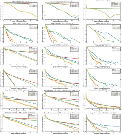
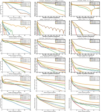
In this section, we conduct various experiments to study the effect of the Catalyst accel-eration and its different variants, showing in particular how to accelerate SVRG, SAGA, and MISO. In Section 5.1, we describe the data sets and formulations considered for our evaluation, and in Section 5.2, we present the different variants of Catalyst. Then, we study different questions: which variant of Catalyst should we use for incremental ap-proaches? (Section 5.3); how do various incremental methods compare when accelerated with Catalyst? (Section 5.4); what is the effect of Catalyst on the test error when Catalyst is used to minimize a regularized empirical risk? (Section 5.5); is the theoretical value for κ appropriate? (Section 5.6). The code used for all our experiments is available at
https://github.com/hongzhoulin89/Catalyst-QNing/.
5.1 Data sets, Formulations, and Metric
Data sets. We consider six machine learning data sets with different characteristics in terms of size and dimension to cover a variety of situations.
name covtype alpha real-sim rcv1 MNIST-CKN CIFAR-CKN
n 581 012 250 000 72 309 781 265 60 000 50 000
d 54 500 20 958 47 152 2 304 9 216