Murat Cetin

C

opyright © 2017 by Academic Publishing House Researcher s.r.o.

Published in Slovak Republic

European Journal of Economic Studies

Has been issued since 2012. ISSN: 2304-9669

E-ISSN: 2305-6282

2017, 6(2): 85-95

DOI: 10.13187/es.2017.6.85

www.ejournal2.com

Does Government Size Affect Economic Growth in Developing Countries? Evidence from Non-stationary Panel Data

Murat Cetin a ,*

a _{Namik Kemal University, Turkey}

Abstract

The Armey curve suggests that there is an inverted U relationship between government size and economic growth. In order to investigate this relationship for 12 developing countries from 1990 to 2012, this study uses panel data methodology including panel unit root, cointegration and causality tests. The results show that i) the series are integrated at order of I(1), ii) there exists a long run equilibrium relationship between the variables, iii) economic growth is positively correlated with the government consumption expenditure, iv) economic growth is negatively correlated with the squares of government consumption expenditure, v) there exists a causality running from the explanotary variables to economic growth in the long run and short run. The study provides an evidence that there exists an inverted U relationship between government consumption expenditure and economic growth implying the validity of Armey curve in these countries. The study may also provide some policy implications.

Keywords: government size, economic growth, Armey curve, panel data analysis.

1. Introduction

Economic growth and its determinants has been one of the main topics investigated by theorists and politicians. According to growth literature, there are two fundamental kinds of growth theory. The first is the neoclassical growth theory. It is well known as the exogenous growth model presented by Solow (1956), Swan (1956), and Koopmans (1965). The second is the new growth theory developed by Romer (1986; 1990), Lucas (1988), Barro (1990), Rebelo (1991), Grossman and Helpman (1991), Aghion and Howitt (1992), and Jones (1996). This theory is also known as the endogenous growth model.

The neoclassical theory of growth generally focuse on capital accumulation and its relation to savings and population growth. It suggests that in the long run economy will reach a steady state where per capita output is constant. It also suggests that there is a linear relationship between a number of variables and economic growth in the long-run. According to this theory, government policy cannot influence the steady-state growth rates. As a result, the impact of government policy on the long run growth has not been investigated in this model.

The new growth theory suggests that both transition and steady state growth rates are endogenous and there are several determinants of long run growth. Here, long run growth rates can differ across countries and convergence in income per capita cannot occur. However, according

* _{Corresponding author}

to this theory government policy can affect economic growth either directly or indirectly. In this model there are three basic fiscal instrument affecting the long run growth rates: expenditure, taxation and the aggregate budgetary balance. Firstly, these instruments affect the efficiency of resource use and the rate of factor accumulation. These developments influences a country’s long-run growth performance (Barro, 1989; 1990; Brons et al. 1999).

A part of the new growth theory focuses on the relationship between government size and economic growth. The literature on public expenditure and economic growth stresses on the presence of a historical relationship between government size and GDP growth. This is called as the Armey curve (Armey, 1995), Rahn curve (Rahn and Fox, 1996) or BARS curve (Barro, 1989; Armey, 1995; Rahn and Fox, 1996; Scully, 1994). This literature uses the form of an inverted U-shaped curve. The Armey curve is based on the law of diminishing factor returns and implies the idea that there is a positive correlation between public expenditure and GDP up to a certain point. After that the correlation becomes negative. In other words, after this point an increase in public expenditure leads to a decrease in GDP. So, Armey curve exhibits a relationship similar to that of Kuznets’ curve. According to Armey curve, the government size and economic growth may be modelled by using a quadratic function (Vedder and Gallaway, 1998).

Barro (1990) investigates the impact of different sizes of government on economic growth. According to Barro, an increase in taxes decreases economic growth, while an increase in government expenditure raises marginal productivity of capital. So, economic growth increases. If the government is small, the second force dominates. If the government is large, the first force dominates. The study’s main finding reveals that the relation between government expenditure and economic growth is non-monotonic.

The Armey curve can be formulized in different shapes in order to test whether an “inverted U” relationship exists between public expenditure and economic growth. The empirical research on this topic aims to test the presence of this relationship in different countries by using several econometric techniques. Examples are given by Miller and Russek (1997), Vedder and Gallaway (1998), Kneller et al. (1999), Folster and Henrekson (2001), Pevcin (2004), Chen and Lee (2005), Angelopoulos et al. (2008), Herath (2010), Magazzino and Forte (2010), Afonso and Furceri (2010), Wu et al. (2010), Ijeoma and O’Neal (2012), Roy (2012), and Altunc and Aydın (2013). But, the empirical literature provides inconclusive findings regarding the relationship between government expenditure and economic growth.

Miller and Russek (1997) investigate the link between government expenditure and economic growth in both developed and developing countries. The results indicate that debt-financed increases in government expenditure slow economic growth and tax-financed increases enhance economic growth for developing countries. The results also indicate that there is no relation between debt-financed increases in government expenditure and economic growth and there is negative link between tax-financed increases and economic growth for developed countries.

Vedder and Gallaway (1998) test the validity of the Armey curve in the cases of United States, Sweden, Denmark, Canada, Britain and Italy over the period 1947-1997. The results show that there is empirical evidence supporting the validity of the Armey curve for all these countries. Employing panel data for 22 OECD countries, Kneller et al. (1999) show that productive government expenditure increases economic growth, while non-productive government expenditure does not.

Folster and Henrekson (2001) investigate the impacts of expenditure and fiscal measures on economic growth for rich countries over the period 1970-1995. The study finds a strong negative relationship between public expenditure and economic growth. Using panel data regression analysis based on five-year arithmetic averages, Pevcin (2004) examines the relationship between government expenditure and economic growth for European countries. The empirical findings support the presence of the Armey curve over the period.

Angelopoulos et al. (2008) analyze the relation between government spending and economic growth in developed and developing countries. Using a panel OLS and 2SLS, they find evidence that there is a nonlinear link between government expenditure and economic growth. The results show that an efficient public sector has a positive impact on economic growth.

Herath (2010) investigates the relationship between government expenditure and economic growth in the case of Sri Lanka by using second degree polynomial regressions. The findings show that there is a positive relation between the variables. The findings also support the Armey’s idea of aquadratic curve for Sri Lanka.

Magazzino and Forte (2010) investigate the existence of Armey curve for the EU countries in the period 1970-2009 by using time-series and panel data techniques. The study provides empirical evidences generally supporting the presence of Armey curve.

Afonso and Furceri (2010) analyze the impacts of size and volatility of government revenue and spending on economic growth in OECD and EU countries by applying panel regression analyses. The findings suggest that both variables are harmful to economic growth. In particular, the results show that government consumption and investments have a negative effect on economic growth.

Wu et al. (2010) examine the causal relation between government spending and economic growth by using the panel Granger causality method presented by Hurlin (2004) and panel data set from 1950 to 2004. The study finds evidence of a positive relation between government spending and economic growth. The sudy also finds bi-directional causality between the variables for the different sub samples of countries.

Ijeoma and O’Neal (2012) examine the impact of government expenditure on economic growth for Nigerian economy from 1980 to 2011. Using ARDL bounds testing approach, the results indicate that government recurrent and capital expenditures are positively correlated with economic growth in the short-run. In the long run there is a positive relation between government recurrent expenditure and economic growth, while government capital expenditure is negatively linked to economic growth in Nigeria.

Using time-series data covering the period 1950-2007, Roy (2012) analyses the relationship between government size and economic growth in the United States. The study particularly investigates the impacts of government consumption and government investment expenditures on US economic growth. Based on the results of a simultaneous-equation model, government consumption expenditure decreases economic growth, while government investment expenditure increases economic growth in the United States. So, the study shows that the overall impact of total government spending on economic growth is uncertain.

Altunc and Aydın (2013) examine the presence of Armey curve for Turkey, Romania and Bulgaria by using ARDL bounds testing approach to cointegration from 1995 to 2011. This study finds an empirical evidence that the Armey curve is valid for Turkey, Romania and Bularia.

Following the empirical lietrature, this study’s main aim is to investigate wether the Armey curve (the inverted U relationship between government size and economic growth) exists in developing countries over the period 1990-2012. In this purpose, we employ panel unit root tests developed by Maddala and Wu (1999), Hadri (2000), and Im et al. (2003). We also employ the cointegration methods developed by Kao (1999) and Maddala and Wu (1999) to examine the long-run relationship between the variables. Long-long-run estimation is conducted by panel OLS method. Finally, the long run and short run causality between the variables is investigated by panel vector error correction model (PVECM).

The remainder of this study is organized as follows. Section 2 describes the model and data of the empirical analysis. Section 3 presents the empirical methodology. Empirical results are reported in Section 4. Section 5 concludes the study with some policy implications.

2. Model and Data

government size and economic growth (Armey curve), the following quadratic function presented by Vedder and Gallaway (1998) can be used

it it it

it

LNGOV

LNGOV

LNGDP





₀





₁





₂ 2





₍₁₎

where GDP, GOV and GOV2 _{represent per capita real income, government consumption}

expenditure as a percentage of real GDP and square of government consumption expenditure as a percentage of annual real GDP, respectively. So, government consumption expenditure is used as an indicator of government size. The data are transformed to natural logarithm because log-linear form provides a better result. α1 and α2 are the slope coefficients and the sign of the coefficients is

expected to be positive and negative, repectively (Vedder and Gallaway, 1998; Herath, 2010; Altunc and Aydın, 2013). εt is the error term assumed to be normally distributed with zero mean and

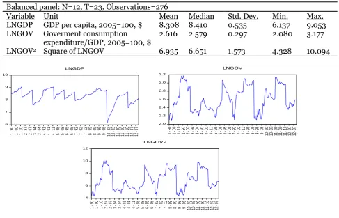
constant variance. Table 1 presents the descriptive statistics of the variables employed in the analysis. Figure 1 shows the plots of the series.

Table 1. Descriptive statistics

Balanced panel: N=12, T=23, Observations=276

Variable Unit Mean Median Std. Dev. Min. Max.

LNGDP GDP per capita, 2005=100, $ 8.308 8.410 0.535 6.137 9.053

LNGOV Goverment consumption

expenditure/GDP, 2005=100, $ 2.616 2.579 0.297 2.080 3.177

LNGOV2 _{Square of LNGOV 6.935 6.651 1.573 4.328 10.094}

6 7 8 9 10 1 - 90 1 - 00 1 - 10 2 - 97 2 - 07 3 - 94 3 - 04 4 - 91 4 - 01 4 - 11 5 - 98 5 - 08 6 - 95 6 - 05 7 - 92 7 - 02 7 - 12 8 - 99 8 - 09 9 - 96 9 - 06 1 0 - 9 3 1 0 - 0 3 1 1 - 9 0 1 1 - 0 0 1 1 - 1 0 1 2 - 9 7 1 2 - 0 7 LNGDP 2.0 2.2 2.4 2.6 2.8 3.0 3.2 1 - 90 1 - 00 1 - 10 2 - 97 2 - 07 3 - 94 3 - 04 4 - 91 4 - 01 4 - 11 5 - 98 5 - 08 6 - 95 6 - 05 7 - 92 7 - 02 7 - 12 8 - 99 8 - 09 9 - 96 9 - 06 1 0 - 9 3 1 0 - 0 3 1 1 - 9 0 1 1 - 0 0 1 1 - 1 0 1 2 - 9 7 1 2 - 0 7 LNGOV 4 6 8 10 12 1 - 90 1 - 00 1 - 10 2 - 97 2 - 07 3 - 94 3 - 04 4 - 91 4 - 01 4 - 11 5 - 98 5 - 08 6 - 95 6 - 05 7 - 92 7 - 02 7 - 12 8 - 99 8 - 09 9 - 96 9 - 06 1 0 - 9 3 1 0 - 0 3 1 1 - 9 0 1 1 - 0 0 1 1 - 1 0 1 2 - 9 7 1 2 - 0 7 LNGOV2

Fig. 1. The plots of LNGDP, LNGOV and LNGOV2 _series

3. Econometric Methodology

3.1 Panel Unit Root Tests

Im et al. (2003) provides a very simple panel unit root test which is well known as IPS test. They employ a separate ADF regression as follows:

∑

1 , 1

,

i p

j

it j t i ij t

i i i

it

y

y

y



 





















(2)

where i = 1, . . .,N and t = 1, . . .,T

The test allows for a heterogeneous coefficient of yit-1 and bases on averaging individual unit

root test statistics. In this test, the null and alternative hypotheses are as follows:

0 :

0 i 

H



for all i (3)

0

:

1 i

H



for i = 1, 2, ….. N1

(4)H₁:



_i 0for i = N1+1, ….. N (5)

The IPS t-bar statistic indicates an average of the individual ADF statistics and is estimated as follows:







N

i i

NT

t

N

t

1

1

 (6)

where t𝞺i is the individual t-statistic for testing H0 hypothesis. In case the lag order is always

zero, IPS provides simulated critical values related with t-bar for different number of cross-sections N and series lenght T. IPS reveals that standardized t-bar statistic exhibits an asymptotic N(0,1) distribution.

The unit root test developed by Maddala and Wu (1999) uses the Fisher (p) test. Under cross-sectional independence of the error terms εit, the joint test statistic can be expressed as follows:









N

i i

p

1

)

ln(

2



(7)

In this procedure, the null and alternative hypotheses are similar to IPS’s hypotheses. Using the ADF estimation equation in each cross-section, this test computes the ADF t-statistic for each individual series. So, the Fisher-test statistics are calculated and are compared with the appropriate χ2 _{critical value.}

Hadri (2000) presents a panel version of the Kwiatkowski et al. (1992) test. In this procedure, the null hypothesis implies that there exists stationarity in all units. The null hypothesis is tested against the alternative of a unit root in all units. The test is based on Langrange multiplier test and the residuals are obtained from the following regression:

it mt mi

it d

y 







, m = 2, 3 for i = 1, …… N. (8)

The test statistic is then given by





 



T

t ei

it N

i LM

S

NT

H

1 2 2

1 2

_ˆ

1

with





T_

t it

ei

e

T

1

2 2

1

_ˆ

ˆ



.

3.2 Panel Cointegration Tests

Kao (1999) suggests several residual-based panel tests and they have parametric properties. In these tests, the null hypothesis implies that there exsists no cointegration. In this procedure, the DF and ADF unit root tests are added to panel cointegration analyses. The main feature of these tests is that they base on the spurious least squares dummy variable panel regression equation as follows:

it it i

it e

y 









 , i = 1,……N; t = 1,…….T (10)

in which 



t_

s is

it u

y

1 and 





t

s is

it x

1



are restricted to be atmost I(1) with uit∼ (0, 2

u



) i.i.d.

and εit∼ (0,



2_{) i.i.d.. The ADF type panel statistic developed by Kao bases on the following AR (p)}

regression itp p t i p t i t i

it pe e e v

eˆ  ˆ,_1



1ˆ,_1...



ˆ,_  (11)

Kao (1999) formulates the ADF panel test statistic as follows:





2 0 2 2 2 0 0 1 ' 1 '

ˆ

10

ˆ

3

ˆ

2

ˆ

ˆ

2

ˆ

6

)

(

)

(

v v v v v v sv N

i i i i

N

i i i i

N

e

Q

e

v

Q

e

ADF























  (12)

where ' 1 '

)

(

_{ip ip ip}

ip

i

I

X

X

X

X

Q





 , and

X

_ipindicates a matrix of observations on the

regressors (eˆi,t1,eˆi,t2,...,eˆi,tp).

NT v s N i T t itp v

 

 

 1 1 2

2 ˆ ₍₁₃₎

where

v

ˆ

_itpimplies the estimate of

v

_itp. The panel ADF test has a asymptotically N(0,1)

distribution.

Hence, in addition to the Kao test, we also employ Fisher’s test to aggregate the p-values of the individual Johansen maximum likelihood cointegration test statistics. In the Fisher procedure which is a non-parametric test the homogeneity in the coefficients are not assumed (Maddala and Kim, 1998; Maddala and Wu, 1999).

3.3 Panel Granger Causality Test

it it q

k

q

k

q

k

k it ik

k it ik

k it ik

it LNGDP LNGOV LNGOV ECT

LNGDP 







 



 



 







 _

     







1

1 1 1

2 3

2 1

1 (14)

where  and q represent the first difference operator and the lag length, respectively. ECT denotes the error-correction term which contains estimated residuals from the cointegration regression (Eq. 1). μ is the serially uncorrelated error term. γ reflects the long-run equilibrium relationship among the variables. If θ2 or θ3 is not equal to zero, it is determined to be a short run

causal relationship. If γ is not equal to zero, it is determined to be a long run causal relationship. If γ and θ2 or θ3 are not equal to zero, it is determined to be a joint causal relationship.

4. Empirical Findings

Table 2 reports panel unit root test results. The findings indicate that the series are not stationary in level. After taking the first difference, the series are stationary. So, it is concluded that all variables are integrated at order of I(1). These results enable us to apply the cointegration tests.

Table 2. Panel unit root test results

Notes: The optimal lag lengths are selected automatically using Akaike information criteria (AIC). The LLC test uses Newey-West bandwidth selection with Bartlett kernel. a _{denotes significance at} the 1 % level. p-values are given in parentheses.

Table 3 presents the results of Johasen-Fisher and Kao cointegration tests. Fisher statistics estimated from trace and maximum eigen tests indicate that there are two cointegration vectors implying the presence of a long-run relationship between the variables at the %1 level. Kao test results indicate the existence of a long-run relationship between te variables. All the findings provide an evidence that there is a cointegration relationship between per capita real income, government consumption expenditure and square of government consumption expenditure over the period.

Variables IPS

test statistics

ADF-Fisher

test statistics test statistics PP-Fisher Hadri test statistics

Panel A: Level

LNGDP 4.576 5.851 5.293 11.799a_0.000

LNGOV -0.805 29.220 21.627 8.704a_0.000

LNGOV2 _{-0.727 28.713 21.981 8.784}a_0.000

Panel B: First difference

ΔLNGDP

-9.257a_0.000

122.139a_0.000 _133.135a_0.000 0.645

ΔLNGOV

-9.481a_0.000

128.351a_0.000 _145.549a_0.000 0.092

ΔLNGOV2

-9.199a_0.000 124.941

Table 3. Panel cointegration test results

Notes: The optimal lag length is selected using AIC. a _and b _{denote significance at the 1% and 5% level,} respectively. The values in parenthesis are p-values.

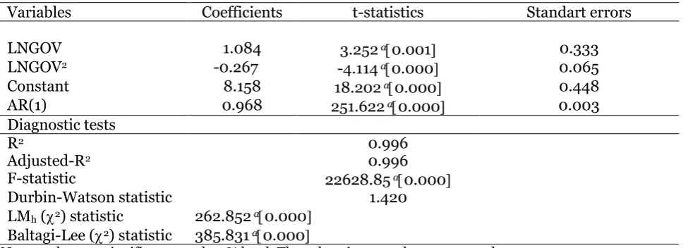
The estimations of long-run parameters are conducted by using panel pooled OLS method. The results are presented in Table 4. Diagnostic tests show that there are the problems of serial correlation and heteroscedasticity in the model. We apply the processes of AR(1) and White cross-section to resolve these problems. The results show that economic growth is positively correlated with the government consumption expenditure. This indicate that an increase in government size can enhance economic growth. The results also show that economic growth is negatively correlated with the square of government consumption expenditure. These findings provide an evidence supporting the presence of an inverted U shaped relationship between government size and economic growth.

Table 4. Panel regression estimation results

(Dependent variable: LNGDP, Method: Pooled panel OLS)

Variables Coefficients t-statistics Standart errors

LNGOV 1.084 3.252 a_{0.001 0.333}

LNGOV2 _{-0.267 -4.114} a_0.000 0.065

Constant 8.158 18.202 a_0.000 0.448

AR(1) 0.968 251.622 a_{0.000 0.003}

Diagnostic tests

R2 _0.996

Adjusted-R2 _0.996

F-statistic 22628.85 a_0.000

Durbin-Watson statistic 1.420

LMh (2) statistic 262.852 a0.000

Baltagi-Lee (2_{) statistic 385.831} a_0.000

Notes: a _{denotes significance at the 1% level. The values in parentheses are p-values}

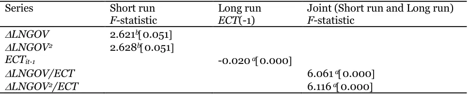
Table 5 reports the results of the long-run, short-run and joint Granger causality. The results suggest that the lagged error correction term is negative and statistically significant at 5 % level as expected. This implies a causality running from government consumption expenditure and the squares of government consumption expenditure to economic growth in the long run. It is found that there exists a causal relation running from government consumption expenditure and the squares of government consumption expenditure to economic growth in the short run. It is also found that there exists a joint causal relation running from the explanatory variables to economic growth. The Granger causality findings provide an evidence that government consumption expenditure (government size) causes economic growth in developing countries over the period.

Cointegration tests Fisher statistics

(from trace test) (from max. eigen test) Fisher statistics

Panel A: Johansen-Fisher

None 255.6a_0.000 _195.8a_0.000

At most 1 121.0a_0.000 _120.0a_0.000

At most 2 32.880.106 32.880.106

Panel B: Kao ADF statistics

Table 5. Panel Granger causality test results (Dependent variable: LNGDP)

Series Short run

F-statistic Long run ECT(-1) Joint (Short run and Long run) F-statistic LNGOV 2.621b_0.051

LNGOV2 _2.628b_0.051

ECTit-1 -0.020 a0.000

LNGOV/ECT 6.061 a_0.000

LNGOV2_{/ECT 6.116} a_0.000

Notes: The optimal lag length is selected using AIC. a _and b _{denote significance at the 1 % and 5 % level,} respectively. The values in parentheses are p-values.

5. Conclusion and Policy Implication

The determinants of economic growth have been discussed by theorists and econometricians for a long time. Growth literature presents two fundemental models: exogenous growth model and endogenous growth model. The first model suggests that there is a linear relationship between a number of variables and economic growth in the long-run. In this model, government policy cannot influence the steady-state growth rates. The second model is well known as new growth theory. In this model government policy can affect economic growth either directly or indirectly. In this contex, a fundemental strand of the new growth theory concentrates on the inverted U relationship between government size and economic growth. This is generally called as Armey curve.

The study investigates the cointegration and causal relationship between the government consumption expenditure and economic growth in the context of Armey curve. We employ panel data covering 1990-2012 for 12 developing countries. Panel unit root tests indicate that the series are integrated at order of I(1) implying that we can apply the cointegration tests. Panel cointegration tests reveal that there exists a lon run relationship between the variables. Panel pooled OLS estimations suggest that the coefficients of government consumption expenditure and the squares of government consumption expenditure are positive and negative, respectively as expected. Granger causality test based on VECM shows that there exists a causal relation running from government consumption expenditure and the squares of government consumption expenditure to economic growt in the long run and short run. All the empirical findings reveal that there exists an inverted U-shaped relationship between government consumption expenditure and economic growth. So, the study provides an empirical evidence that the Armey curve is valid for developing countries over the period.

The empirical results also imply that there is an optimal level of government consumption expenditure. Therefore, governments should avoid excessive consumption expenditure. Otherwise, these excessive expenditure hamper to economic growth. On the other hand, this study can be repeated by considering different kinds of government spending. This empirical study may also bring about new empirical studies. In this respect, a further empirical research may include the individual countries or the sub groups of the panel.

References

Afonso, Furceri, 2010 – Afonso, A., Furceri, D. (2010). Government size, composition, volatility and economic growth. European Journal of Political Economy, 26, 517-532.

Altunc, Aydın, 2013 – Altunc, O. F., Aydın, C. (2013). The relationship between optimal size

of government and economic growth: Empirical evidence from Turkey, Romania and Bulgaria. Procedia-Social and Behavioral Sciences, 92, 66-75.

Angelopoulos, Philippopoulos, Tsionas, 2008 – Angelopoulos, K., Philippopoulos, A.,

Tsionas, E. (2008). Does public sector efficiency matter? Revisiting the relation between fiscal size and economic growth in a world sample. Public Choice, 137, 245-278.

Armey, 1995 – Armey, D. (1995). The Freedom Revolution, Regnery Publishing Co., Washington, D.C.

Barro, 1990 – Barro, R.J. (1990). Government spending in a simple model of endogenous growth. Journal of Political Economy, 98(5), 103-125.

Brons, de Groot, Nijkamp, 1999 – Brons, M., de Groot, H.L.F., Nijkamp, P. (1999). Growth effects of fiscal policies. Tinbergen Discussion Paper, Amsterdam: Vrije Universiteit.

Chen, Lee, 2005 – Chen, S.T., Lee, C.C. (2005). Government size and economic growth in Taiwan: A threshold regression approach. Journal of Policy Modeling, 27, 1051-1066.

Folster, Henrekson, 2001 – Folster, S., Henrekson, F. (2001). Growth effects of government expenditure and taxation in rich countries. European Economic Review, 45(8), 1501-1520.

Grossman, Helpman, 1991 – Grossman, G.M., Helpman, E. (1991). Quality ladders in the theory of growth. Review of Economic Studies, 58(1), 43-61.

Hadri, 2000 – Hadri, K. (2000). Testing for stationarity in heterogeneous panel data. Econometric Journal, 3, 148-161.

Herath, 2010 – Herath, S. (2010). The size of the government and economic growth: An empirical study of Sri Lanka. SRE-Discussion Papers, 2010/05. WU Vienna University of Economics and Business, Vienna.

Ijeoma, O’Neal, 2012 – Ijeoma, E.K., O’Neal, E.J. (2012). Government expenditure and economic growth in Nigeria, 1980-2011. International Journal of Academic Research, 4(6), 205-209.

Im, Pesaran, Shin, 2003 – Im, K.S., Pesaran, M.H., Shin, Y. (2003). Testing for unit roots in heterogeneous panels. Journal of Econometrics, 115, 53-74.

Jones, 1995 – Jones, C.I. (1995). Time series tests of endogenous growth models. Quarterly Journal of Economics, 110(2), 495-525.

Kao, 1999 – Kao, C. (1999). Spurious regression and residual-based tests for cointegration in panel data. Journal of Econometrics, 90, 1-44.

Kneller, Bleaney, Gemmell, 1998 – Kneller, R., Bleaney, M.F., Gemmell, N. (1998). Growth, public policy and the government budget constraint: Evidence from OECD countries. Discussion Paper No.98/14, School of Economics, University of Nottingham.

Koopmans, 1965 – Koopmans, T.C. (1965). On the Concept of Optimal Economic Growth. The Econometric Approach to Development Planning, North-Holland, Amsterdam.

Kwiatkowski, Phillips, Schmidt, Shin, 1992 – Kwiatkowski, D., Phillips, P. C. B., Schmidt, P., Shin, Y. (1992). Testing for the null of stationarity against the alternative of a unit root. Journal of Econometrics, 54, 159-178.

Lucas, 1988 – Lucas, R. (1988). On the mechanics of economic development. Journal of Monetary Economics, 22, 2-42.

Maddala, Wu, 1999 – Maddala, G.S., Wu, S. (1999). A comparative study of unit root tests with panel data and a new simple test. Oxford Bulletin of Economics and Statistics, 61, 631-52.

Maddala, Kim, 1998 – Maddala, G.S., Kim, I.M. (1998). Unit Roots, Cointegration, and Structural Change. Cambridge University Press, Cambridge.

Magazzino, Forte, 2010 – Magazzino, C., Forte, F. (2010). Optimal size of government and economic growth in EU-27. MPRA Paper, No. 26669.

Miller, Russek, 1997 – Miller, S.M., Russek, F.S. (1997). Fiscal structures and economic growth: International evidence. Economic Inquiry, 35(3), 603-613.

Pevcin, 2004 - Pevcin, P. (2004). Does Optimal Spending Size of Government Exist?. EGPA-European Group of Public Administration, Katholieke Universiteit Leuven, Belgium, Retrieved August 18, 2008, from http://soc.kuleuven.be/io/egpa/fin/paper/slov2004 /pevcin.pdf

Rahn, Fox, 1996 – Rahn, R., Fox, H. (1996). What Is the Optimum Size of Government?. Vernon K. Krieble Foundation.

Rebelo, 1991 – Rebelo, S. (1991). Long-run policy analysis and long-run growth. Journal of Political Economy, 99(June), 500-521.

Romer, 1986 – Romer, P.M. (1986). Increasing returns and long-run growth. Journal of Political Economy, 94(5), 1002-1037.

Romer, 1990 – Romer, P.M. (1990). Endogenous technological change. Journal of Political Economy, 98(5), 71-102.

Scully, 1994 – Scully, G.W. (1994). What is the Optimal Size of Government in the US?. National Center for Policy Analysis, Policy Report 188.

Solow, 1956 – Solow, R. (1956). A contribution to the theory of economic growth. Quarterly Journal of Economics, 70, 65-94.

Swan, 1956 – Swan, T. (1956). Economic growth and capital accumulation. Economic Record, 32(Nov), 334-361.

Vedder, Gallaway, 1998 – Vedder, R.K., Gallaway, L.E. (1998). Government size and economic growth. paper prepared for the Joint Economic Committee, Retrieved September 11, 2008, from http://www.house.gov/jec/growth/function/function.pdf

World Bank, 2016 – World Bank, (2016). World Development Indicators. http://data.worldbank.org/data-catalog/world-development-indicators