Learning Permutations with Exponential Weights
∗David P. Helmbold [email protected]
Manfred K. Warmuth† [email protected]
Computer Science Department University of California, Santa Cruz Santa Cruz, CA 95064
Editor: Yoav Freund
Abstract
We give an algorithm for the on-line learning of permutations. The algorithm maintains its un-certainty about the target permutation as a doubly stochastic weight matrix, and makes predictions using an efficient method for decomposing the weight matrix into a convex combination of per-mutations. The weight matrix is updated by multiplying the current matrix entries by exponential factors, and an iterative procedure is needed to restore double stochasticity. Even though the re-sult of this procedure does not have a closed form, a new analysis approach allows us to prove an optimal (up to small constant factors) bound on the regret of our algorithm. This regret bound is sig-nificantly better than that of either Kalai and Vempala’s more efficient Follow the Perturbed Leader algorithm or the computationally expensive method of explicitly representing each permutation as an expert.
Keywords: permutation, ranking, on-line learning, Hedge algorithm, doubly stochastic matrix,
relative entropy projection, Sinkhorn balancing
1. Introduction
Finding a good permutation is a key aspect of many problems such as the ranking of search results or matching workers to tasks. In this paper we present an efficient and effective on-line algorithm for learning permutations in a model related to the on-line allocation model of learning with experts (Freund and Schapire, 1997). In each trial, the algorithm probabilistically chooses a permutation and then incurs a linear loss based on how appropriate the permutation was for that trial. The regret is the total expected loss of the algorithm on the whole sequence of trials minus the total loss of the best permutation chosen in hindsight for the whole sequence, and the goal is to find algorithms that have provably small worst-case regret.
For example, one could consider a commuter airline which owns n airplanes of various sizes and flies n routes.1 Each day the airline must match airplanes to routes. If too small an airplane is assigned to a route then the airline will loose revenue and reputation due to unserved potential passengers. On the other hand, if too large an airplane is used on a long route then the airline could have larger than necessary fuel costs. If the number of passengers wanting each flight were known ahead of time, then choosing an assignment is a weighted matching problem. In the on-line
∗. An earlier version of this paper appears in Proceedings of the Twentieth Annual Conference on Computational
Learn-ing Theory (COLT 2007), published by SprLearn-inger as LNAI 4539.
allocation model, the airline first chooses a distribution over possible assignments of airplanes to routes and then randomly selects an assignment from the distribution. The regret of the airline is the earnings of the single best assignment for the whole sequence of passenger requests minus the total expected earnings of the on-line assignments. When airplanes and routes are each numbered from 1 to n, then an assignment is equivalent to selecting a permutation. The randomness helps protect the on-line algorithm from adversaries and allows one to prove good bounds on the algorithm’s regret for arbitrary sequences of requests.
Since there are n! permutations on n elements, it is infeasible to simply treat each permutation as an expert and apply one of the expert algorithms that uses exponential weights. Previous work has exploited the combinatorial structure of other large sets of experts to create efficient algorithms (see Helmbold and Schapire, 1997; Takimoto and Warmuth, 2003; Warmuth and Kuzmin, 2008, for examples). Our solution is to make a simplifying assumption on the loss function which allows the new algorithm, called PermELearn, to maintain a sufficient amount of information about the distribution over n! permutations while using only n2weights.
We represent a permutation of n elements as an n×n permutation matrix ΠwhereΠi,j=1 if
the permutation maps element i to position j and Πi,j=0 otherwise. As the algorithm randomly
selects a permutationΠb at the beginning of a trial, an adversary simultaneously selects an arbitrary loss matrix L∈[0,1]n×nwhich specifies the loss of all permutations for the trial. Each entry L
i,jof
the loss matrix gives the loss for mapping element i to j, and the loss of any whole permutation is the sum of the losses of the permutation’s mappings, that is, the loss of permutationΠis∑iLi,Π(i)=
∑i,jΠi,jLi,j. Note that the per-trial expected losses can be as large as n, as opposed to the common
assumption for the expert setting that the losses are bounded in[0,1]. In Section 3 we show how a variety of intuitive loss motifs can be expressed in this matrix form.
This assumption that the loss has a linear matrix form ensures the expected loss of the algorithm can be expressed as∑i,jWi,jLi,j, where W =E(Πb). This expectation W is an n×n weight matrix
which is doubly stochastic, that is, it has non-negative entries and the property that every row and column sums to 1. The algorithm’s uncertainty about which permutation is the target is summarized by W ; each weight Wi,j is the probability that the algorithm predicts with a permutation mapping
element i to position j. It is worth emphasizing that the W matrix is only a summary of the distribu-tion over permutadistribu-tions used by any algorithm (it doesn’t indicate which permutadistribu-tions have non-zero probability, for example). However, this summary is sufficient to determine the algorithm’s expected loss when the losses of permutations have the assumed loss matrix form.
Our PermELearn algorithm stores the weight matrix W and must convert W into an efficiently sampled distribution over permutations in order to make predictions. By Birkhoff’s Theorem, ev-ery doubly stochastic matrix can be expressed as the convex combination of at most n2−2n+2 permutations (see, e.g., Bhatia, 1997). In Appendix A we show that a greedy matching-based al-gorithm efficiently decomposes any doubly stochastic matrix into a convex combination of at most n2−2n+2 permutations. Although the efficacy of this algorithm is implied by standard dimension-ality arguments, we give a new combinatorial proof that provides independent insight as to why the algorithm finds a convex combination matching Birkhoff’s bound. Our algorithm for learning per-mutations predicts with a randomΠbsampled from the convex combination of permutations created by decomposing weight matrix W . It has been applied recently for pricing combinatorial markets when the outcomes are permutations of objects (Chen et al., 2008).
Warmuth, 1994; Vovk, 1990; Freund and Schapire, 1997): each entry Wi,j is multiplied by a factor
e−ηLi,j. Hereηis a positive learning rate that controls the “strength” of the update (Whenη=0,
than all the factors are one and the update is vacuous). After this update, the weight matrix no longer has the doubly stochastic property, and the weight matrix must be projected back into the space of doubly stochastic matrices (called “Sinkhorn balancing”, see Section 4) before the next prediction can be made.
In Theorem 4 we bound the expected loss of PermELearn over any sequence of trials by
n ln n+η
L
best1−e−η , (1)
where n is the number of elements being permuted,ηis the learning rate, and
L
best is the loss ofthe best permutation on the entire sequence. If an upper bound
L
est≥L
best is known, thenηcanbe tuned (as in Freund and Schapire, 1997) and the expected loss bound becomes
L
best+p2L
estn ln n+n ln n, (2)giving a bound ofp2
L
estn ln n+n ln n on the worst case expected regret of the tuned PermELearn algorithm. We also prove a matching lower bound (Theorem 6) ofΩ(pL
bestn ln n)for the expected regret of any algorithm solving our permutation learning problem.A simpler and more efficient algorithm than PermELearn maintains the sum of the loss matrices on the the previous trials. Each trial it adds random perturbations to the cumulative loss matrix and then predicts with the permutation having minimum perturbed loss. This “Follow the Perturbed Leader” algorithm (Kalai and Vempala, 2005) has good regret bounds for many on-line learning settings. However, the regret bound we can obtain for it in the permutation setting is about a factor of n worse than the bound for PermELearn and the lower bound.
Although computationally expensive, one can also consider running the Hedge algorithm while explicitly representing each of the n! permutations as an expert. If T is the sum of the loss matrices over the past trials and F is the n×n matrix with entries Fi,j =e−ηTi,j, then the weight of each
permutation expert Π is proportional to the product ∏iFi,Π(i) and the normalization constant is
the permanent of the matrix F. Calculating the permanent is a known #P-complete problem and sampling from this distribution over permutations is very inefficient (Jerrum et al., 2004). Moreover since the loss range of a permutation is[0,n], the standard loss bound for the algorithm that uses one expert per permutation must be scaled up by a factor of n, becoming
L
best+nr
2
L
estn ln(n!) +n ln(n!)≈
L
best+q
2
L
estn2ln n+n2ln n.This expected loss bound is similar to our expected loss bound for PermELearn in Equation (2), ex-cept that the n ln n terms are replaced by n2ln n. Our method based on Sinkhorn balancing bypasses the estimation of permanents and somehow PermELearn’s implicit representation and prediction method exploit the structure of permutations and lets us obtain the improved bound. We also give a matching lower bound that shows PermELearn has the optimum regret bound (up to a small constant factor). It is an interesting open question whether the structure of permutations can be exploited to prove bounds like (2) for the Hedge algorithm with one expert per permutation.
factor are the derivatives of our linear loss with respect to the weights Wi,j. This family of
up-dates usually maintains a probability vector as its weight vector. In that case the normalization of the weight vector is straightforward and is folded directly into the update formula. Our new algo-rithm PermELearn for learning permutations maintains a doubly stochastic matrix with n2weights. The normalization alternately normalizes the rows and columns of the matrix until convergence (Sinkhorn balancing). This may require an unbounded number of steps and the resulting matrix does not have a closed form. Despite this fact, we are able to prove bounds for our algorithm.
We first show that our update minimizes a tradeoff between the loss and a relative entropy between doubly stochastic matrices. This relative entropy becomes our measure of progress in the analysis. Luckily, the un-normalized multiplicative update already makes enough progress (towards the best permutation) to achieve the loss bound quoted above. Finally, we interpret the iterations of Sinkhorn balancing as Bregman projections with respect to the same relative entropy and show using the properties of Bregman projections that these projections can only increase the progress and thus don’t hurt the analysis (Herbster and Warmuth, 2001).
Our new insight of splitting the update into an un-normalized step followed by a normalization step also leads to a streamlined proof of the loss bound for the Hedge algorithm in the standard expert setting that is interesting in its own right. Since the loss in the allocation setting is linear, the bounds can be proven in many different ways, including potential based methods (see, e.g., Kivinen and Warmuth, 1999; Gordon, 2006; Cesa-Bianchi and Lugosi, 2006). For the sake of completeness we reprove our main loss bound for PermELearn using potential based methods in Appendix B. We show how potential based proof methods can be extended to handle linear equality constraints that don’t have a solution in closed form, paralleling a related extension to linear inequality constraints in Kuzmin and Warmuth (2007). In this appendix we also discuss the relationship between the projection and potential based proof methods. In particular, we show how the Bregman projection step corresponds to plugging in suboptimal dual variables into the potential.
The remainder of the paper is organized as follows. We introduce our notation in the next section. Section 3 presents the permutation learning model and gives several intuitive examples of appropriate loss motifs. Section 4 gives the PermELearn algorithm and discusses its computational requirements. One part of the algorithm is to decompose the current doubly stochastic matrix into a small convex combination of permutations using a greedy algorithm. The bound on the number of permutations needed to decompose the weight matrix is deferred to Appendix A. We then bound PermELearn’s regret in Section 5 in a two-step analysis that uses a relative entropy as a measure of progress. To exemplify the new techniques, we also analyze the basic Hedge algorithm with the same methodology. The regret bounds for Hedge and PermELearn are re-proven in Appendix B using potential based methods. In Section 6, we apply the “Follow the Perturbed Leader” algorithm to learning permutations and show that the resulting regret bounds are not as good. In Section 7 we prove a lower bound on the regret when learning permutations that is within a small constant factor of our regret bound on the tuned PermELearn algorithm. The concluding section describes extensions and directions for further work.
2. Notation
All matrices will be n×n matrices. When A is a matrix, Ai,j denotes the entry of A in row i, and
column j. We use A•B to denote the dot product between matrices A and B, that is,∑i,jAi,jBi,j. We
Permutations on n elements are frequently represented in two ways: as a bijective mapping of the elements {1, . . . ,n}into the positions {1, . . . ,n} or as a permutation matrix which is an n×n binary matrix with exactly one “1” in each row and each column. We use the notationΠ(andΠb) to represent a permutation in either format, using the context to indicate the appropriate representation. Thus, for each i∈ {1, . . . ,n}, we useΠ(i)to denote the position that the ith element is mapped to by permutationΠ, and matrix elementΠi,j=1 ifΠ(i) = j and 0 otherwise.
If L is a matrix with n rows then the productΠL permutes the rows of L:
Π=
0 1 0 0
0 0 0 1
0 0 1 0
1 0 0 0
L=
11 12 13 14 21 22 23 24 31 32 33 34 41 42 43 44
ΠL=
21 22 23 24 41 42 43 44 31 32 33 34 11 12 13 14
.
perm.(2,4,3,1)as matrix an arbitrary matrix permuting the rows
Convex combinations of permutations create doubly stochastic or balanced matrices: non-negative matrices whose n rows and n columns each sum to one. Our algorithm maintains its uncertainty about which permutation is best as a doubly stochastic weight matrix W and needs to randomly select a permutation from some distribution whose expectation is W . By Birkhoff’s The-orem (see, e.g., Bhatia, 1997), for every doubly stochastic matrix W there is a decomposition into a convex combination of at most n2−2n+2 permutation matrices. We show in Appendix A how a decomposition of this size can be found effectively. This decomposition gives a distribution over permutations whose expectation is W that now can be effectively sampled because its support is at most n2−2n+2 permutations.
3. On-line Protocol
We are interested in learning permutations in a model related to the on-line allocation model of learning with experts (Freund and Schapire, 1997). In that model there are N experts and at the beginning of each trial the algorithm allocates a probability distribution w over the experts. The algorithm picks expert i with probability wi and then receives a loss vectorℓ∈[0,1]N. Each expert
i incurs loss ℓi and the expected loss of the algorithm is w·ℓ. Finally, the algorithm updates its distribution w for the next trial.
In case of permutations we could have one expert per permutation and allocate a distribution over the n! permutations. Explicitly tracking this distribution is computationally expensive, even for moderate n. As discussed in the introduction, we assume that the losses in each trial can be specified by a loss matrix L∈[0,1]n×n where the loss of each permutation Πhas the linear form ∑iLi,Π(i)=Π•L. If the algorithm’s predictionΠb is chosen probabilistically in each trial then the
algorithm’s expected loss is E[Πb•L] =W•L, where W =E[Πb]. This expected prediction W is an n×n doubly stochastic matrix and algorithms for learning permutations under the linear loss assumption can be viewed as implicitly maintaining such a doubly stochastic weight matrix.
More precisely, the on-line algorithm follows the following protocol in each trial:
• The learner (probabilistically) chooses a permutationΠb, and let W =E(Πb).
• Nature simultaneously chooses a loss matrix L∈[0,1]n×nfor the trial.
• Finally, the algorithm updates its distribution over permutations for the next trial, implicitly updating matrix W .
Although our algorithm can handle arbitrary sequences of loss matrices L∈[0,1]n×n, nature
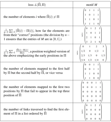
could be significantly more restricted. Many ranking applications have an associated loss motif M and nature is constrained to choose (row) permutations of M as its loss matrix L. In effect, at each trial nature chooses a “correct” permutation Π and uses the loss matrix L=ΠM. Note that the permutation left-multiplies the loss motif, and thus permutes the rows of M. If nature chooses the identity permutation then the loss matrix L is the motif M itself. When M is known to the algorithm, it suffices to give the algorithm only the permutationΠat the end of the trial, rather than the loss matrix L itself. Figure 1 gives examples of loss motifs.
The last loss in Figure 1 is related to a competitive List Update Problem where an algorithm services requests to a list of n items. In the List Update Problem the cost of a request is the requested item’s current position in the list. After each request, the requested item can be moved forward in the list for free, and additional rearrangement can be done at a cost of one per transposition. The goal is for the algorithm to be cost-competitive with the best static ordering of the elements in hindsight. Note that the transposition cost for additional list rearrangement is not represented in the permutation loss motif. Blum et al. (2003) give very efficient algorithms for the List Update Problem that do not do additional rearranging of the list (and thus do not incur the cost neglect by the loss motif). In our notation, their bound has the same form as ours (1) but with the n ln n factors replaced by O(n). However, our lower bound (see Section 7) shows that the n ln n factors in (2) are necessary in the general permutation setting.
Note that many compositions of loss motifs are possible. For example, given two motifs with their associated losses, any convex combination of the motifs creates a new motif for the same convex combination of the associated losses. Other component-wise combinations of two motifs (such as product or max) can also produce interesting loss motifs, but the combination usually cannot be distributed across the matrix dot-product calculation, and so cannot be expressed as a simple linear function of the original losses.
4. PermELearn Algorithm
Our permutation learning algorithm uses exponenential weights and we call it PermELearn. It maintains an n×n doubly stochastic weight matrix W as its main data structure, where Wi,j is the
probability that PermELearn predicts with a permutation mapping element i to position j. In the absence of prior information it is natural to start with uniform weights, that is, the matrix with 1n in each entry.
In each trial PermELearn does two things:
1. Choose a permutationΠb from some distribution such thatE[Πb] =W .
loss
L
(Πb,Π) motif Mthe number of elements i whereΠb(i)6=Π
0 1 1 1 1 0 1 1 1 1 0 1 1 1 1 0
1
n−1∑
n
i=1|Πb(i)−Π(i)|, how far the elements are from their “correct” positions (the division by n− 1 ensures that the entries of M are in[0,1].)
1 3
0 1 2 3 1 0 1 2 2 1 0 1 3 2 1 0
1
n−1∑
n i=1|
b Π(i)−Π(i)|
Π(i) , a position weighted version of
the above emphasizing the early positions inΠ
1 3
0 1 2 3
1/2 0 1/2 1 2/3 1/3 0 1/3 3/4 1/2 1/4 0
the number of elements mapped to the first half byΠbut the second half byΠb, or vice versa
0 0 1 1 0 0 1 1 1 1 0 0 1 1 0 0
the number of elements mapped to the first two positions byΠthat fail to appear in the top three position ofΠb
0 0 0 1 1 0 0 0 1 1 0 0 0 0 0 0 0 0 0 0 0 0 0 0 0
the number of links traversed to find the first ele-ment ofΠin a list ordered byΠb
1 3
0 1 2 3 0 0 0 0 0 0 0 0 0 0 0 0
Figure 1: Loss motifs
Choosing a permutation is done by Algorithm 1. The algorithm greedily decomposes W into a convex combination of at most n2−2n+2 permutations (see Theorem 7), and then randomly selects one of these permutations for the prediction.2
Our decomposition algorithm uses a Temporary matrix A initialized to the weight matrix W . Each iteration of Algorithm 1 finds a permutationΠwhere each Ai,Π(i)>0. This can be done by
finding a perfect matching on the n×n bipartite graph containing the edge i,j whenever Ai,j >0.
We shall soon see that each matrix A is a constant times a doubly stochastic matrix, so the existence of a suitable permutation Πfollows from Birkhoff’s Theorem. Given such a permutation Π, the algorithm updates A to A−αΠ where α=miniAi,Π(i). The updated matrix A has non-negative
entries and has strictly more zeros than the original A. Since the update decreases each row and
Algorithm 1 PermELearn: Selecting a permutation Require: a doubly stochastic n×n matrix W
A :=W ; q=0; repeat
q :=q+1;
Find permutationΠqsuch that Ai,Πq(i)is positive for each i∈ {1, . . . ,n}
αq:=miniAi,Πq(i)
A :=A−αqΠq
until All entries of A are zero {at end of loop W =∑qk=1αkΠk}
Randomly select and return aΠb∈ {Π1, . . . ,Πq}using probabilitiesα
1, . . . ,αq.
Algorithm 2 PermELearn: Weight Matrix Update
Require: learning rateη, loss matrix L, and doubly stochastic weight matrix W
Create W′where each Wi′,j=Wi,je−ηLi,j (3)
Create doubly stochasticW by re-balancing the rows and columns of We ′ (Sinkhorn balancing) and update W toW .e
column sum byα and the original matrix W was doubly stochastic, each matrix A will have rows and columns that sum to the same amount. In other words, each matrix A created during Algorithm 1 is a constant times a doubly stochastic matrix, and thus (by Birkhoff’s Theorem) is a constant times a convex combination of permutations.
After at most n2−n iterations the algorithm arrives at a matrix A having exactly n non-zero entries, so this A is a constant times a permutation matrix. Therefore, Algorithm 1 decomposes the original doubly stochastic matrix into the convex combination of (at most) n2−n+1 permutation matrices. The more refined arguments in Appendix A shows that the Algorithm 1 never uses more than n2−2n+2 permutations, matching the bound given by Birkhoff’s Theorem.
Several improvements are possible. In particular, we need not compute each perfect matching from scratch. If only z entries of A are zeroed by a permutation, then that permutation is still a matching of size n−z in the graph for the updated matrix. Thus we need to find only z augmenting paths to complete the perfect matching. The entire process thus requires finding O(n2)augmenting paths at a cost of O(n2)each, for a total cost of O(n4)to decompose weight matrix W into a convex combination of permutations.
4.1 Updating the Weights
In the second step, Algorithm 2 updates the weight matrix by multiplying each Wi,j entry by the
factor e−ηLi,j. These factors destroy the row and column normalization, so the matrix must be
1 2 1 2 1 2 1 ! Sinkhorn balancing =⇒ √ 2 1+√2
1 1+√2 1
1+√2
√
2 1+√2
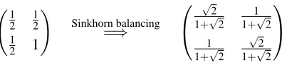
Figure 2: Example where Sinkhorn balancing requires infinitely many steps.
Normalizing the rows corresponds to pre-multiplying by a diagonal matrix. The product of these diagonal matrices thus represents the combined effect of the multiple row normalization steps. Sim-ilarly, the combined effect of the column normalization steps can be represented by post-multiplying the matrix by a diagonal matrix. Therefore we get the well known fact that Sinkhorn balancing a matrix A results in a doubly stochastic matrix RAC where R and C are diagonal matrices. Each entry Ri,iis the positive multiplier applied to row i, and each entry Cj,jis the positive multiplier of column
j needed to convert A into a doubly stochastic matrix.
In Figure 2 we give a rational matrix that balances to an irrational matrix. Since each row and column balancing step creates rationals, Sinkhorn balancing produces irrationals only in the limit (after infinitely many steps). Multiplying a weight matrix from the left and/or right by non-negative diagonal matrices (e.g., row or column normalization) preserves the ratio of product weights be-tween permutations. That is if A′=RAC, then for any two permutationsΠ1andΠ2,
∏iA′i,Π1(i) ∏iA′i,Π2(i)
= ∏iAi,Π1(i)Ri,iCΠ1(i),Π1(i) ∏iAi,Π2(i)Ri,iCΠ2(i),Π2(i)
=∏iAi,Π1(i)
∏iAi,Π2(i) . Therefore 1/2 1/2 1/2 1
must balance to a doubly stochastic matrix 1−aa1−aasuch that the ratio of the product weight between the two permutations(1,2)and(2,1)is preserved. This means1/21/4=(1−a2a)2
and thus a= √2 1+√2.
This example leads to another important observation: PermELearn’s predictions are different than Hedge’s when each permutation is treated as an expert. If each permutation is explicitly repre-sented as an expert, then the Hedge algorithm predicts permutationΠwith probability proportional to the product weight, ∏ie−η∑t
Lt
i,Π(i). However, algorithm PermELearn predicts differently. With
the weight matrix in Figure 4.1, Hedge puts probability 23 on permutation(1,2)and probability 13 on permutation(2,1) while PermELearn puts probability
√
2
1+√2 ≈0.59 on permutation(1,2)and probability √1
1+√2≈0.41 on permutation (2,1).
There has been much written on the balancing of matrices, and we briefly describe only a few of the results here. Sinkhorn showed that this procedure converges and that the RAC balancing of any matrix A into a doubly stochastic matrix is unique (up to canceling multiples of R and C) if it exists3(Sinkhorn, 1964).
A number of authors consider balancing a matrix A so that the row and column sums are 1±ε. Franklin and Lorenz (1989) show that O(length(A)/ε)Sinkhorn iterations suffice, where length(A)
is the bit-length of matrix A’s binary representation. Kalantari and Khachiyan (1996) show that
3. Some non-negative matrices, like 10 11 00
0 1 1
, cannot be converted into doubly stochastic matrices because of their
O(n4lnnεlnmin A1
i,j) operations suffice using an interior point method. Linial et al. (2000) give a
preprocessing step after which only O((n/ε)2) Sinkhorn iterations suffice. They also present a strongly polynomial time iterative procedure requiring ˜O(n7log(1/ε))iterations. Balakrishnan et al. (2004) give an interior point method with complexity O(n6log(n/ε)). Finally, F¨urer (2004) shows that if the row and column sums of A are 1±εthen every matrix entry changes by at most ±nε when A is balanced to a doubly stochastic matrix.
4.2 Dealing with Approximate Balancing
With slight modifications, Algorithm PermELearn can handle the situation where its weight matrix is imperfectly balanced (and thus not quite doubly stochastic). As before, let W be the fully balanced doubly stochastic weight matrix, but we now assume that only an approximately balanced W isb available to predict from. In particular, we assume that each row and column ofW sum to 1b ±εfor someε< 1
3. Let s≥1−εbe the smallest row or column sum inW .b
We modify Algorithm 1 in two ways. First, A is initialized to 1sW rather than W . This ensuresb every row and column in the initial A sums to at least one, to at most 1+3ε, and at least one row or column sums to exactly 1. Second, the loop exits as soon as A has an all-zero row or column. Since the smallest row or column sum starts at 1, is decreased byαk each iteration k, and ends at
zero, we have that∑qk=1αk=1 and the modified Algorithm 1 still outputs a convex combination of
permutations C=∑qk=1αkΠk. Furthermore, each entry Ci,j≤ 1sWbi,j. We now bound the additional
loss of this modified algorithm.
Lemma 1 If the weight matrixW is approximately balanced so each row and column sum is in 1b ±ε (forε≤ 13) then the modified Algorithm 1 has an expected loss C•L at most 3n3εgreater than the expected loss W•L of the original algorithm that uses the completely balanced doubly stochastic matrix W .
Proof Let s be the smallest row or column sum inW . Since each row and column sum ofb 1sWb lies in[1,1+3ε], each entry of 1sW is close to the corresponding entry of the fully balanced W . Inb particular each 1sWbi,j≤Wi,j+3nε(F¨urer, 2004). This allows us to bound the expected loss when
predicting with the convex combination C in terms of the expected loss using a decomposition of the perfectly balanced W :
C•L ≤ 1 sWb•L
=
∑
i,j b
Wi,j
s Li,j
≤
∑
i,j
(Wi,j+3nε)Li,j
≤ W•L+3n3ε.
If in a sequence of T trials the matricesW areb ε=1/(3T n3) balanced (so that each row and column sum is 1±1/(3T n3)) then Lemma 1 implies that the total additional expected loss for using approximate balancing is at most 1. The algorithm of Balakrishnan et al. (2004)ε-balances a matrix in O(n6log(n/ε))time (note that this dominates the time for the loss update and constructing the convex combination). This balancing algorithm withε=1/(3T n3)together with the modified prediction algorithm give a method requiring O(T n6log(T n))total time over the T trials and having a bound ofp2
L
estn ln n+n ln n+1 on the worst-case regret.If the number of trials T is not known in advance then settingεas a function of t can be helpful. A natural choice isεt =1/(3t2n3). In this case the total extra regret for not having perfect balancing
is bounded by∑Tt=11/t2≤5/3 and the total computation time over the T trials is still bounded by O(T n6log(T n)).
One might be concerned about the effects of approximate balancing propagating between trials. However this is not an issue. In the following section we show that the loss updates and balancing can be arbitrarily interleaved. Therefore the modified algorithm can either keep a cumulative loss matrix L≤t =∑t
i=1Li and create its nextW by (approximately) balancing the matrix with entriesb 1
ne−
ηL≤i,jt, or apply the multiplicative updates to the previous approximately balancedW .b
5. Bounds for PermELearn
Our analysis of PermELearn follows the entropy-based analysis of the exponentiated gradient family of algorithms (Kivinen and Warmuth, 1997). This style of analysis first shows a per-trial progress bound using relative entropy to a comparator as a measure of progress, and then sums this invariant over the trials to bound the expected total loss of the algorithm. We also show that PermELearn’s weight update belongs to the exponentiated gradient family of updates (Kivinen and Warmuth, 1997) since it is the solution to a minimization problem that trades of the loss (in this case a linear loss) against a relative entropy regularization.
Recall that the expected loss of PermELearn on a trial is a linear function of its weight matrix W . Therefore the gradient of the loss is independent of the current value of W . This property of the loss greatly simplifies the analysis. Our analysis for this setting provides a good foundation for learning permutation matrices and lays the groundwork for the future study of other permutation loss functions.
We start our analysis with an attempt to mimic the standard analysis (Kivinen and Warmuth, 1997) for the exponentiated gradient family updates which multiply by exponential factors and re-normalize. The per-trial invariant used to analyze the exponentiated gradient family bounds the decrease in relative entropy from any (normalized) vector u to the algorithm’s weight vector by a linear combination of the algorithm’s loss and the loss of u on the trial. In our case the weight vectors are matrices and we use the following (un-normalized) relative entropy between matrices A and B with non-negative entries:
∆(A,B) =
∑
i,j
Ai,jln
Ai,j
Bi,j
+Bi,j−Ai,j .
Note that this is just the sum of the relative entropies between the corresponding rows (or equiva-lently, between the corresponding columns):
∆(A,B) =
∑
i
∆(Ai,⋆,Bi,⋆) =
∑
j
(here Ai,⋆is the ith row of A and A⋆,j is its jth column).
Unfortunately, the lack of a closed form for the matrix balancing procedure makes it difficult to prove bounds on the loss of the algorithm. Our solution is to break PermELearn’s update (Algo-rithm 2) into two steps, and use only the progress made to the intermediate un-balanced matrix in our per-trial bound (8). After showing that balancing to a doubly stochastic matrix only increases the progress, we can sum the per-trial bound to obtain our main theorem.
5.1 A Dead End
In each trial, PermELearn multiplies each entry of its weight matrix by an exponential factor and then uses one additional factor per row and column to make the matrix doubly stochastic (Algo-rithm 2 described in Section 4.1):
e
Wi,j:=ricjWi,je−ηLi,j (4)
where the riand cj factors are chosen so that all rows and columns of the matrixW sum to one.e
We now show that PermELearn’s update (4) gives the matrix A solving the following minimiza-tion problem:
argmin ∀i :∑jAi,j=1
∀j :∑iAi,j=1
(∆(A,W) +η(A•L)). (5)
Since the linear constraints are feasible and the divergence is strictly convex, there always is a unique solution, even though the solution does not have a closed form.
Lemma 2 PermELearn’s updated weight matrixW (4) is the solution of (5).e
Proof We form a Lagrangian for the optimization problem:
l(A,ρ,γ) =∆(A,W) +η(A•L) +
∑
i ρi(
∑
j
Ai,j−1) +
∑
jγj(
∑
iAi,j−1).
Setting the derivative with respect to Ai,j to 0 yields Ai,j=Wi,je−ηLi,je−ρie−γj. By enforcing the
row and column sum constraints we see that the factors ri=e−ρi and cj=e−γj function as row and
column normalizers, respectively.
We now examine the progress ∆(U,W)−∆(U,We) towards an arbitrary stochastic matrix U . Using Equation (4) and noting that all three matrices are doubly stochastic (so their entries sum to n), we see that
∆(U,W)−∆(U,We) =−ηU•L+
∑
i
ln ri+
∑
jln cj.
Making this a useful invariant requires lower bounding the sums on the rhs by a constant times W•L, the loss of the algorithm. Unfortunately we are stuck because the ri and cj normalization
5.2 Successful Analysis
Our successful analysis splits the update (4) into two steps:
Wi′,j:=Wi,je−ηLi,j and Wei,j:=ricjWi′,j, (6)
where (as before) ri and cj are chosen so that each row and column of the matrixW sum to one.e
Using the Lagrangian (as in the proof of Lemma 2), it is easy to see that these W′ andW matricese solve the following minimization problems:
W′=argmin
A
(∆(A,W) +η(A•L)) and W :e = argmin ∀i :∑jAi,j=1
∀j :∑iAi,j=1
∆(A,W′). (7)
The second problem shows that the doubly stochastic matrixW is the projection of We ′ onto to the linear row and column sum constraints. The strict convexity of the relative entropy between non-negative matrices and the feasibility of the linear constraints ensure that the solutions for both steps are unique.
We now lower bound the progress∆(U,W)−∆(U,W′)in the following lemma to get our per-trial invariant.
Lemma 3 For anyη>0, any doubly stochastic matrices U and W and any trial with loss matrix L∈[0,1]n×n
∆(U,W)−∆(U,W′)≥(1−e−η)(W•L)−η(U•L),
where W′is the unbalanced intermediate matrix (6) constructed by PermELearn from W .
Proof The proof manipulates the difference of relative entropies and uses the inequality e−ηx≤ 1−(1−e−η)x, which holds for anyηand any x∈[0,1]:
∆(U,W)−∆(U,W′) =
∑
i,j
Ui,jln
Wi′,j Wi,j
+Wi,j−Wi′,j
=
∑
i,j
Ui,jln(e−ηLi,j) +Wi,j−Wi,je−ηLi,j
≥
∑
i,j
−ηLi,jUi,j+Wi,j−Wi,j(1−(1−e−η)Li,j)
= −η(U•L) + (1−e−η)(W•L).
Relative entropy is a Bregman divergence, so the Generalized Pythagorean Theorem (Bregman, 1967) applies. Specialized to our setting, this theorem states that if S is a closed convex set contain-ing some matrix U with non-negative entries, W′is any matrix with strictly positive entries, andWe is the relative entropy projection of W′onto S then
Furthermore, this holds with equality when S is affine, which is the case here since S is the set of matrices whose rows and columns each sum to 1. Rearranging and noting that∆(A,B)is non-negative yields Corollary 3 of Herbster and Warmuth (2001), which is the inequality we need:
∆(U,W′)−∆(U,We) =∆(We,W′)≥0.
Combining this with the inequality of Lemma 3 gives the critical per-trial invariant:
∆(U,W)−∆(U,We)≥(1−e−η)(W•L)−η(U•L). (8)
We now introduce some notation and bound the expected total loss by summing the above inequality over a sequence of trials. When considering a sequence of trials, Lt is the loss matrix at trial t, Wt−1 is PermELearn’s weight matrix W at the start of trial t (so W0 is the initial weight matrix) and Wtis the updated weight matrixW at the end of the trial.e
Theorem 4 For any learning rate η>0, any doubly stochastic matrices U and initial W0, and any sequence of T trials with loss matrices Lt ∈[0,1]n×n (for 1≤t ≤T ), the expected loss of
PermELearn is bounded by:
T
∑
t=1
Wt−1•Lt≤ ∆(U,W
0)−∆(U,WT) +η∑T
t=1U•Lt
1−e−η .
Proof Applying (8) to trial t gives:
∆(U,Wt−1)−∆(U,Wt)≥(1−e−η)(Wt−1•Lt)−η(U•Lt).
By summing the above over all T trials we get:
∆(U,W0)−∆(U,WT)≥(1−e−η)
T
∑
t=1
Wt−1•Lt−η
T
∑
t=1 U•Lt.
The bound then follows by solving for the total expected loss,∑Tt=1Wt−1•Lt, of the algorithm.
When the entries of W0 are all initialized to 1n and U is a permutation then∆(U,W0) =n ln n. Since each doubly stochastic matrix U is a convex combination of permutation matrices, at least one minimizer of the total loss∑Tt=1U•L will be a permutation matrix. If
L
best denotes the loss ofsuch a permutation U∗, then Theorem 4 implies that the total loss of the algorithm is bounded by
∆(U∗,W0) +η
L
best
1−e−η .
If upper bounds ∆(U∗,W0)≤Dest ≤n ln n and
L
est≥L
best are known, then by choosing η=ln
1+
r
2Dest
Lest
, and the above bound becomes (Freund and Schapire, 1997):
L
best+p2L
estDest+∆(U∗,W0). (9)A natural choice for Dest is nlnn. In this case the tuned bound becomes
5.3 Approximate Balancing
The preceding analysis assumes that PermELearn’s weight matrix is perfectly balanced each itera-tion. However, balancing techniques are only capably of approximately balancing the weight matrix in finite time, so implementations of PermELearn must handle approximately balanced matrices. In Section 4.2, we describe an implementation that uses an approximately balancedWbt−1at the start of iteration t rather than the completely balanced Wt−1of the preceding analysis. Lemma 1 shows that when this implementation of PermELearn uses an approximately balancedWbt−1 where each row and column sum is in 1±εt, then the expected loss on trial t is at most Wt−1•Lt+3n3εt. Summing
over all trials and using Theorem 4, this implementation’s total loss is at most
T
∑
t=1
Wt−1•Lt+3n3εt
≤∆(U,W
0)−∆(U,WT) +η∑T
t=1U•Lt
1−e−η +
T
∑
t=1 3n3εt .
As discussed in Section 4.2, settingεt =1/(3n3t2)leads to an additional loss of less than 5/3
over the bound of Theorem 4 and its subsequent tunings while incurring a total running time (over all T trials) in O(T n6log(T n)). In fact, the additional loss for approximate balancing can be made less than any positive c by settingεt =c/(5n3t2). Since the time to approximately balance depends
only logarithmically on 1/ε, the total time taken over T trials remains in O(T n6log(T n)).
5.4 Split Analysis for the Hedge Algorithm
Perhaps the simplest case where the loss is linear in the parameter vector is the on-line allocation setting of Freund and Schapire (1997). It is instructive to apply our method of splitting the update in this simpler setting. There are N experts and the algorithm keeps a probability distribution w over the experts. In each trial the algorithm picks expert i with probability wi and then gets a loss
vectorℓ∈[0,1]N. Each expert i incurs lossℓiand the algorithm’s expected loss is w·ℓ. Finally w is
updated tow for the next trial.e
The Hedge algorithm (Freund and Schapire, 1997) updates its weight vector to ˜wi= wie
−ηℓi
∑jwje−ηℓj
.
This update can be motivated by a tradeoff between the un-normalized relative entropy to the old weight vector and expected loss in the last trial (Kivinen and Warmuth, 1999):
e
w :=argmin ∑iwbi=1
(∆(wb,w) +ηwb·ℓ).
For vectors, the relative entropy is simply∆(bw,w):=∑iwbilnwwbii+wi−wbi.As in the permutation
case, we can split this update (and motivation) into two steps: setting each w′i=wie−ηℓi thenwe=
w′/∑iw′i. These are the solutions to:
w′:=argmin
b w
(∆(wb,w) +ηwb·ℓ) and w :e =argmin ∑iwbi=1
The following lower bound has been shown on the progress towards any probability vector u serving as a comparator:4
∆(u,w)−∆(u,ew) = −ηu·ℓ−ln
∑
i
wie−ηℓi
≥ −ηu·ℓ−ln
∑
i
wi(1−(1−e−η)ℓi)
≥ −ηu·ℓ+w·ℓ(1−e−η), (10)
where the first inequality uses e−ηx≤1−(1−e−η)x, for any x∈[0,1], and the second uses−ln(1−
x)≥x, for x∈[0,1].Surprisingly the same inequality already holds for the un-normalized update:5
∆(u,w)−∆(u,w′) =−ηu·ℓ+
∑
i
wi(1−e−ηℓi)≥w·ℓ(1−e−η)−ηu·ℓ.
Since the normalization is a projection w.r.t. a Bregman divergence onto a linear constraint satisfied by the comparator u,∆(u,w′)−∆(u,we)≥0 by the Generalized Pythagorean Theorem (Herbster and Warmuth, 2001). The total progress for both steps is again Inequality (10).
With the key Inequality (10) in hand, it is easy to introduce trial dependent notation and sum over trails (as done in the proof of Theorem 4, arriving at the familiar bound for Hedge (Freund and Schapire, 1997): For anyη>0, any probability vectors w0and u, and any loss vectorsℓt ∈[0,1]n,
T
∑
t=1
wt−1•ℓt≤ ∆(u,w
0)−∆(u,wT) +η∑T t=1u•ℓt
1−e−η . (11)
Note that the r.h.s. is actually constant in the comparator u (Kivinen and Warmuth, 1999), that is, for all u,
∆(u,w0)−∆(u,wT) +η∑Tt=1u•ℓt
1−e−η =
−ln∑iw0ie−ηℓ
≤T i
1−eη .
The r.h.s. of the above equality is often used as a potential in proving bounds for expert algorithms. We discuss this further in Appendix B.
5.5 When to Normalize?
Probably the most surprising aspect about the proof methodology is the flexibility about how and when to project onto the constraints. Instead of projecting a nonnegative matrix onto all 2n con-straints at once (as in optimization problem (7)), we could mimic the Sinkhorn balancing algorithm by first projecting onto the row constraints and then the column constraints and alternating until convergence. The Generalized Pythagorean Theorem shows that projecting onto any convex con-straint that is satisfied by the comparator class of doubly stochastic matrices brings the weight matrix closer to every doubly stochastic matrix.6 Therefore our bound on∑tWt−1•Lt (Theorem 4) holds
if the exponential updates are interleaved with any sequence of projections to some subsets of the
4. This is essentially Lemma 5.2 of Littlestone and Warmuth (1994). The reformulation of this type of inequality with relative entropies goes back to Kivinen and Warmuth (1999)
5. Note that if the algorithm does not normalize the weights then w is no longer a distribution. When∑iwi<1, the loss
w·L amounts to incurring 0 loss with probability 1−∑iwi, and predicting as expert i with probability wi.
constraints. However, if the normalization constraints are not enforced then W is no longer a convex combination of permutations. Furthermore, the exponential update factors only decrease the entries of W and without any normalization all of the entries of W can get arbitrarily small. If this is al-lowed to happen then the “loss” W•L can approach 0 for any loss matrix, violating the spirit of the prediction model.
There is a direct argument that shows that the same final doubly stochastic matrix is reached if we interleave the exponential updates with projections to any of the constraints as long as all 2n constraints hold at the end. To see this we partition the class of matrices with positive entries into equivalence classes. Call two such matrices A and B equivalent if there are diagonal matrices R and C with positive diagonal entries such that B=RAC. Note that[RAC]i,j=Ri,iAi,jCj,j and therefore
B is just a rescaled version of A. Projecting onto any row and/or column sum constraints amounts to pre- and/or post-multiplying the matrix by some positive diagonal matrices R and C. Therefore if matrices A and B are equivalent then the projection of A (or B) onto a set of row and/or column sum constraints results in another matrix equivalent to both A and B.
The importance of equivalent matrices is that they balance to the same doubly stochastic matrix.
Lemma 5 For any two equivalent matrices A and RAC, where the entries of A and the diagonal entries of R and C are positive,
argmin ∀i :∑jAbi,j=1
∀j :∑iAbi,j=1
∆(Ab,A) = argmin
∀i :∑jAbi,j=1
∀j :∑iAbi,j=1
∆(Ab,RAC).
Proof The strict convexity of the relative entropy implies that both problems have a unique matrix as their solution. We will now reason that the unique solutions for both problems are the same. By using a Lagrangian (as in the proof of Lemma 2) we see that the solution of the left optimization problem is a square matrix with ˙riAi,jc˙j in position i,j. Similarly the solution of the problem on
the right has ¨riRi,iAi,jCj,jc¨j in position i,j. Here the factors ˙ri,¨ri function as row normalizers and
˙
cj,c¨j as column normalizers. Given a solution matrix ˙ri,c˙j to the left problem, then ˙ri/Ri,i,c˙j/Cj,j
is a solution of the right problem of the same value. Also if ¨ri,c¨j is a solution of right problem, then
¨riRi,i,c¨jCj,j is a solution to the left problem of the same value.
This shows that both minimization problems have the same value and the matrix solutions for both problems are the same and unique (even though the normalization factors ˙ri,c˙j of say the left
problem are not necessarily unique). Note that its crucial for the above argument that the diagonal entries of R,C are positive.
The analogous phenomenon is much simpler in the weighted majority case: Two non-negative vectors a and b are equivalent if a=cb, where c is any nonnegative scalar, and again each equiva-lence class has exactly one normalized weight vector.
PermELearn’s intermediate matrix Wi′,j:=Wi,je−ηLi,j can be written W◦M where◦denotes the
Hadamard (entry-wise) Product and Mi,j =e−ηLi,j. Note that the Hadamard product commutes
with matrix multiplication by diagonal matrices, if C is diagonal and P= (A◦B)C then Pi,j =
(Ai,jBi,j)Cj,j= (Ai,jCj,j)Bi,jso we also have P= (AC)◦B. Similarly, R(A◦B) = (RA)◦B when R
Hadamard products also preserve equivalence. For equivalent matrices A and B=RAC (for diagonal R and C) the matrices A◦M and B◦M are equivalent (although they are not likely to be equivalent to A and B) since B◦M= (RAC)◦M=R(A◦M)C.
This means that any two runs of PermELearn-like algorithms that have the same bag of loss matrices and equivalent initial matrices end with equivalent final matrices even if they project onto different subsets of the constraints at the end of the various trials.
In summary the proof method discussed so far uses a relative entropy as a measure of progress and relies on Bregman projections as its fundamental tool. In Appendix B we re-derive the bound for PermELearn using the value of the optimization problem (5) as a potential. This value is expressed using the dual optimization problem and intuitively the application of the Generalized Pythagorean Theorem now is replaced by plugging in a non-optimal choice for the dual variables. Both proof techniques are useful.
5.6 Learning Mappings
We have an algorithm that has small regret against the best permutation. Permutations are a subset of all mappings from{1, . . . ,n}to{1, . . . ,n}. We continue usingΠfor a permutation and introduce
Ψto denote an arbitrary mapping from{1, . . . ,n}to{1, . . . ,n}. Mappings differ from permutations in that the n dimensional vector(Ψ(i))n
i=1can have repeats, that is,Ψ(i)might equalΨ(j)for i6= j. Again we alternately represent a mappingΨas an n×n matrix whereΨi,j=1 ifΨ(i) = j and 0
otherwise. Note that such square7mapping matrices have the special property that they have exactly one 1 in each row. Again the loss is specified by a loss matrix L and the loss of mappingΨisΨ•L. It is straightforward to design an algorithm MapELearn for learning mappings with exponential weights: Simply run n independent copies of the Hedge algorithm for each of the n rows of the received loss matrices. That is, the r’th copy of Hedge always receives the r’th row of the loss matrix L as its loss vector. Even though learning mappings is easy, it is nevertheless instructive to discuss the differences with PermELearn.
Note that MapELearn’s combined weight matrix is now a convex combination of mappings, that is, a “singly” stochastic matrix with the constraint that each row sums to one. Again, after the exponential update (3), the constraints are typically not satisfied any more, but they can be easily reestablished by simply normalizing each row. The row normalization only needs to be done once in each trial: no iterative process is needed. Furthermore, no fancy decomposition algorithm is needed in MapELearn: for (singly) stochastic weight matrix W , the predictionΨ(i) is simply a random element chosen from the row distribution Wi,∗. This sampling procedure produces a mappingΨ
such that W=E(Ψ)and thusE(Ψ•L) =W•L as needed.
We can use the same relative entropy between the single stochastic matrices, and the lower bound on the progress for the exponential update given in Lemma 3 still holds. Also our main bound (Theorem 4) is still true for MapELearn and we arrive at the same tuned bound for the total loss of MapELearn:
L
best+p2L
estDest+∆(U∗,W0),where
L
best,L
est, and Dest are now the total loss of the best mapping, a known upper bound onL
best, and an upper bound on∆(U∗,W0), respectively. Recall thatL
est and Dest are needed to tunetheηparameter.
Our algorithm PermElearn for permutations may be seen as the above algorithm for mappings while enforcing the column sum constraints in addition to the row constraints used in MapELearn. Since PermELearn’s row balancing “messes up” the column sums and vice versa, an interactive procedure (i.e., Sinkhorn Balancing) is needed to create to a matrix in which each row and col-umn sums to one. The enforcement of the additional colcol-umn sum constraints results in a doubly stochastic matrix, an apparently necessary step to produce predictions that are permutations (and an expected prediction equal to the doubly stochastic weight matrix).
When it is known that the comparator is a permutation, then the algorithm always benefits from enforcing the additional column constraints. In general we should always make use of any constraints that the comparator is known to satisfy (see, e.g., Warmuth and Vishwanathan, 2005, for a discussion of this).
As discussed in Section 4.1, if A′ is a Sinkhorn-balanced version of a non-negative matrix A, then
for any permutationsΠ1andΠ2,
∏iAi,Π1(i) ∏iAi,Π2(i)
=∏iA
′ i,Π1(i) ∏iA′i,Π2(i)
. (12)
An analogous invariant holds for mappings: If A′is a row-balanced version of a non-negative matrix A, then
for any mappingsΨ1andΨ2,
∏iAi,Ψ1(i) ∏iAi,Ψ2(i)
= ∏iA
′ i,Ψ1(i) ∏iA′i,Ψ2(i) .
However it is important to note that column balancing does not preserve the above invariant for mappings. In fact, permutations are the subclass of mappings where invariant 12 holds.
There is another important difference between PermELearn and MapELearn. For MapELearn, the probability of predicting mapping Ψ with weight matrix W is always the product ∏iWi,Ψ(i).
The analogous property does not hold for PermELearn. Consider the balanced 2×2 weight matrix W on the right of Figure 2. This matrix decomposes into √2
1+√2 times the permutation(1,2) plus 1
1+√2 times the permutation (2,1). Thus the probability of predicting with permutation (1,2) is
√
2 times the probability of permutation(2,1)for the PermELearn algorithm. However, when the probabilities are proportional to the intuitive product form∏iWi,Π(i), then the probability ratio for these two permutations is 2. Notice that this intuitive product weight measure is the distribution used by the Hedge algorithm that explicitly treats each permutation as a separate expert. Therefore PermELearn is clearly different than a concise implementation of Hedge for permutations.
6. Follow the Perturbed Leader Algorithm
Perhaps the simplest on-line algorithm is the Follow the Leader (FL) algorithm: at each trial predict with one of the best models on the data seen so far. Thus FL predicts at trial t with an expert in argminiℓ<t
i or any permutation in argminΠΠ•L<t, where “<t” indicates that we sum over the past
trials, that is,ℓ<t
i :=∑tq−=11ℓ
q
i. The FL algorithm is clearly non-optimal; in the expert setting there
is a simple adversary strategy that forces FL to have loss at least n times larger than the loss of the best expert in hindsight.
no ties) and the same holds for PermELearn. Thus the exponential weights with moderateηmay be seen as a soft min calculation: the algorithm hedges its bets and does not put all its probability on the expert with minimum loss so far.
The “Follow the Perturbed Leader” (FPL) algorithm of Kalai and Vempala (2005) is an alternate on-line prediction algorithm that works in a very general setting. It adds random perturbations to the total losses of the experts incurred so far and then predicts with the expert of minimum perturbed loss. Their FPL∗ algorithm has bounds closely related to Hedge and other multiplicative weight algorithms and in some cases Hedge can be simulated exactly (Kuzmin and Warmuth, 2005) by judiciously choosing the distribution of perturbations. However, for the permutation problem the bounds we were able to obtain for FPL∗are weaker than the the bound we obtained bounds for Per-mELearn that uses exponential weights despite the apparent similarity between our representations and the general formulation of FPL∗.
The FPL setting uses an abstract k-dimensional decision space used to encode predictors as well as a k-dimensional state space used to represent the losses of the predictors. At any trial, the current loss of a particular predictor is the dot product between that predictor’s representation in the decision space and the state-space vector for the trial. This general setting can explicitly represent each permutation and its loss when k=n!. The FPL setting also easily handles the encodings of permutations and losses used by PermELearn by representing each permutation matrixΠand loss matrix L as n2-dimensional vectors.
The FPL∗algorithm (Kalai and Vempala, 2005) takes a parameterεand maintains a cumulative loss matrix C (initially C is the zero matrix) At each trial, FPL∗:
1. Generates a random perturbation matrix P where each Pi,j is proportional to±ri,j where ri,j
is drawn from the standard exponential distribution.
2. Predicts with a permutationΠminimizingΠ•(C+P).
3. After getting the loss matrix L, updates C to C+L.
Note that FPL∗ is more computationally efficient than PermELearn. It takes only O(n3) time to make its prediction (the time to compute a minimum weight bipartite matching) and only O(n2)
time to update C. Unfortunately the generic FPL∗ loss bounds are not as good as the bounds on PermELearn. In particular, they show that the loss of FPL∗on any sequence of trials is at most8
(1+ε)
L
best+8n3(1+ln n)
ε
whereεis a parameter of the algorithm. When the loss of the best expert is known ahead of time,ε can be tuned and the bound becomes
L
best+4q
2
L
bestn3(1+ln n) +8n3(1+ln n) .Although FPL∗gets the same
L
best leading term, the excess loss over the best permutation growsas n3ln n rather the n ln n growth of PermELearn’s bound. Of course, PermELearn pays for the improved bound by requiring more computation.