Improving the Reliability of Causal Discovery from Small Data Sets Using Argumentation

Improving the Reliability of Causal Discovery from Small Data Sets

Using Argumentation

Facundo Bromberg [email protected]

Dimitris Margaritis [email protected]

Dept. of Computer Science Iowa State University Ames, IA 50011

Editor: Constantin Aliferis

Abstract

We address the problem of improving the reliability of independence-based causal discovery al-gorithms that results from the execution of statistical independence tests on small data sets, which typically have low reliability. We model the problem as a knowledge base containing a set of inde-pendence facts that are related through Pearl’s well-known axioms. Statistical tests on finite data sets may result in errors in these tests and inconsistencies in the knowledge base. We resolve these inconsistencies through the use of an instance of the class of defeasible logics called argumentation, augmented with a preference function, that is used to reason about and possibly correct errors in these tests. This results in a more robust conditional independence test, called an argumentative

independence test. Our experimental evaluation shows clear positive improvements in the accuracy

of argumentative over purely statistical tests. We also demonstrate significant improvements on the accuracy of causal structure discovery from the outcomes of independence tests both on sampled data from randomly generated causal models and on real-world data sets.

Keywords: independence-based causal discovery, causal Bayesian networks, structure learning, argumentation, reliability improvement

1. Introduction and Motivation

Directed graphical models, also called Bayesian networks, can be used to represent the probability distribution of a domain. This makes them a useful and important tool for machine learning where a common task is inference, that is, predicting the probability distribution of a variable of interest given some other knowledge, usually in the form of values of other variables in the domain. An additional use of Bayesian networks comes by augmenting them with causal semantics that repre-sent cause and effect relationships in the domain. The resulting networks are called causal. An important problem is inferring the structure of these networks, a process that is sometimes called

causal discovery, which can provide insights into the underlying data generation process.

condi-tional independences to constrain the set of possible structures consistent with these to a singleton (if possible) and infer that structure as the only possible one. As such they are called

constraint-based or independence-constraint-based algorithms. In this paper we address open problems related to the

latter class of algorithms.

It is well-known that independence-based algorithms have several shortcomings. A major one has to do with the effect that unreliable independence information has on the their output. In general such independence information comes from two sources: (a) a domain expert that can provide his or her opinion on the validity of certain conditional independences among some of the variables, sometimes with a degree of confidence attached to them, and/or (b) statistical tests of independence, conducted on data gathered from the domain. As expert information is often costly and difficult to obtain, (b) is the most commonly used option in practice. A problem that occurs frequently however is that the data set available may be small. This may happen for various reasons: lack of subjects to observe (e.g., in medical domains), an expensive data-gathering process, privacy concerns and others. Unfortunately, the reliability of statistical tests significantly diminishes on small data sets. For example, Cochran (1954) recommends that Pearson’sχ2independence test be deemed unreli-able if more than 20% of the cells of the test’s contingency tunreli-able have an expected count of less than 5 data points. Unreliable tests, besides producing errors in the resulting causal model struc-ture, may also produce cascading errors due to the way that independence-based algorithms work: their operation, including which test to evaluate next, typically depends on the outcomes of previous ones. Thus a single error in a statistical test can be propagated by the subsequent choices of tests to be performed by the algorithm, and finally when the edges are oriented. Therefore, an error in a previous test may have large (negative) consequences in the resulting structure, a property that is called instability in Spirtes et al. (2000). One possible method for addressing the effect of multiple errors in the construction of a causal model through multiple independence tests is the Bonferroni correction (Hochberg, 1988; Abdi, 2007), which works by dividing the type I error probabilityαof each test by the number of such tests evaluated during the entire execution of the causal learning algorithm. As a result, the collective type I error probability (of all tests evaluated) isα, that is, 0.05 typically. However, this may make the detection of true dependences harder, as now larger data sets would be required to reach the adjusted confidence threshold of each test. The types of adjustments that may be appropriate for each case to tests that may be dependent is an open problem and the subject of current research in statistics (Benjamini and Hochberg, 1995; Benjamini and Yekutieli, 2001; Storey, 2002).

Example 1. Consider an independence-based knowledge base that contains the following

proposi-tions, obtained through statistical tests on data.

({0}⊥⊥{1} | {2}) (1)

({0} 6⊥⊥ {3} | {2}) (2) ({0}⊥⊥{3} | {1,2}) (3)

where(X⊥⊥Y|Z)denotes conditional independence of the set of variables X with Y conditional

on set Z, and(X6⊥⊥Y|Z)denotes conditional dependence. Suppose that (3) is in fact wrong. Such an error can be avoided if there exists a constraint involving these independence propositions. For example, suppose that we also know that the following rule holds in the domain (this is an instance of an application of the Contraction and Decomposition axioms, described later in Section 2):

({0}⊥⊥{1} | {2})∧({0} 6⊥⊥ {3} | {2}) =⇒ ({0} 6⊥⊥ {3} | {1,2}). (4)

Rule (4), together with independence proposition (1) and dependence proposition (2), contradict independence proposition (3), resulting in an inconsistent knowledge base. If Rule (4) and propo-sitions (1) and (2) are accepted, then proposition (3) must be rejected (and its value reversed), correcting the error in this case. The framework presented in the rest of the paper provides a prin-cipled approach for resolving such inconsistencies.

The situation described in the previous example, while simple, illustrates the general idea that we will use in the rest of the paper: the set of independences and dependences used in a causal dis-covery algorithm form a potentially inconsistent knowledge base, and making use of general rules, derived from axioms and theorems that we know hold in the domain, helps us correct certain out-comes of statistical tests. In this way we will be able to improve the reliability of causal discovery algorithms that use them to derive causal models. To accomplish this we use the framework of

argu-mentation, which provides a sound and elegant way of resolving inconsistencies in such knowledge

bases, including ones that contain independences.

2. Notation and Preliminaries

In this work we denote random variables with capitals (e.g., X,Y,Z) and sets of variables with bold

capitals (e.g., X,Y,Z). In particular, we denote by V={1, . . . ,n}the set of all n variables in the domain, naming the variables by their indices in V; for instance, we refer to the third variable in V simply by 3. We assume that all variables in the domain are discrete following a multinomial distribution or are continuous following a Gaussian distribution. We denote the data set by D and its size (number of data points) by N. We use the notation(X⊥⊥Y|Z)to denote that the variables in set X are (jointly) independent of those in Y conditional on the values of the variables in Z, for disjoint sets of variables X, Y, and Z, while(X6⊥⊥Y|Z) denotes conditional dependence. For the sake of readability, we slightly abuse this notation and use(X⊥⊥Y|Z)as shorthand for({X}⊥⊥{Y} | {Z}). A Bayesian network (BN) is a directed graphical model which represents the joint probability distribution over V. Each node in the graph represents one of the random variables in the domain. The structure of the network implicitly represents a set of conditional independences on the domain variables. Given the structure of a BN, the set of independences implied by it can be identified by a process called d-separation (Pearl, 1988); the latter follows from the local Markov property that states that each node in the network is conditionally independent of all its non-descendants in the graph given its parents. All independences identified by d-separation are implied by the model structure. If, in addition, all remaining triplets(X,Y,Z)correspond to dependencies, we say that the BN is directed graph-isomorph (abbreviated DAG-isomorph) or simply causal (as defined by Pearl, 1988). The concept of DAG-isomorphism is equivalent to a property called Faithfulness in Spirtes et al. (2000). A graph G is said to be faithful to some distribution if exactly those independences that exist in the distribution and no others are returned by the process of d-separation on G. In this paper we assume Faithfulness. For learning the structure of the Bayesian network of a domain we make use of the PC algorithm (Spirtes et al., 2000), which is only able to correctly identify the structure under the assumption of causal sufficiency. We therefore also assume causal sufficiency. A domain is causally sufficient if it does not contain any hidden or latent variables.

As mentioned above, independence-based algorithms operate by conducting a series of condi-tional independence queries. For these we assume that an independence-query oracle exists that is able to provide such information. This approach can be viewed as an instance of the statistical query oracle theory of Kearns and Vazirani (1994). In practice such an oracle does not exist, but can be implemented approximately by a statistical test evaluated on the data set (for example, this can be Pearson’s conditional independenceχ2 (chi-square) test (Agresti, 2002), Wilk’s G2 test, a mutual information test etc.). In this work we used Wilk’s G2 test (Agresti, 2002). To determine conditional independence between two variables X and Y given a set Z from data, the statistical test G2(and many other independence tests based on hypothesis testing, for example, theχ2 test) uses the values in the contingency table (a table containing the data point counts for each possible combination of the variables that participate in the test) to compute a test statistic. For a given value of the test statistic, the test then computes the likelihood of obtaining that or a more extreme value by chance under the null hypothesis, which in our case is that the two variables are conditionally independent. This likelihood, called the p-value of the test, is then returned. The p-value of a test equals the probability of falsely rejecting the null hypothesis (independence). Assuming that the p-value of a test is p(X,Y |Z), the statistical test concludes independence if and only if p(X,Y |Z) is greater than a thresholdα, that is,

(Symmetry) (X⊥⊥Y|Z) ⇐⇒ (Y⊥⊥X|Z)

(Decomposition) (X⊥⊥Y∪W|Z) =⇒ (X⊥⊥Y|Z)∧ (X⊥⊥W|Z)

(Weak Union) (X⊥⊥Y∪W|Z) =⇒ (X⊥⊥Y|Z∪W) (5)

(Contraction) (X⊥⊥Y|Z)∧ (X⊥⊥W|Z∪Y) =⇒ (X⊥⊥Y∪W|Z)

(Intersection) (X⊥⊥Y|Z∪W)∧(X⊥⊥W|Z∪Y) =⇒ (X⊥⊥Y∪W|Z)

(Symmetry) (X⊥⊥Y|Z) ⇐⇒ (Y⊥⊥X|Z)

(Composition) (X⊥⊥Y|Z)∧(X⊥⊥W|Z) =⇒ (X⊥⊥Y∪W|Z)

(Decomposition) (X⊥⊥Y∪W|Z) =⇒ (X⊥⊥Y|Z)∧(X⊥⊥W|Z)

(Intersection) (X⊥⊥Y|Z∪W)∧(X⊥⊥W|Z∪Y) =⇒ (X⊥⊥Y∪W|Z)

(Weak Union) (X⊥⊥Y∪W|Z) =⇒ (X⊥⊥Y|Z∪W) (6)

(Contraction) (X⊥⊥Y|Z)∧(X⊥⊥W|Z∪Y) =⇒ (X⊥⊥Y∪W|Z)

(Weak Transitivity) (X⊥⊥Y|Z)∧(X⊥⊥Y|Z∪γ) =⇒ (X⊥⊥γ|Z)∨ (γ⊥⊥Y|Z)

(Chordality) (α⊥⊥β|γ∪δ) ∧(γ⊥⊥δ|α∪β) =⇒ (α⊥⊥β|γ)∨(α⊥⊥β|δ)

Common values in statistics forαare 0.05 and 0.01, corresponding to confidence thresholds(1−α) of 0.95 and 0.99 respectively. The value 0.10 for α is also sometimes used, depending on the application, while values as low as 0.005 and 0.001 are sometimes used for structure learning.

The conditional independences and dependences of a domain are connected through a set of general rules, introduced in Pearl (1988) and shown boxed in Eq. (5). These can be seen as con-straints in a meta-space representing all possible independences in the domain. More specifically, let us imagine a meta-space of binary variables, each corresponding to the truth value of the in-dependence of a triplet(X,Y|Z)(e.g.,truefor independence andfalsefor dependence). Each point in this space corresponds to a conditional independence assignment to all possible triplets in the domain. In this conceptual space not all points are tenable; in particular the set of rules of Eq. (5) constrain the truth values of independences corresponding to triplets. For domains for which there exists a faithful Bayesian network a more relaxed set of properties hold, shown boxed in Eq. (6) whereα,β,γandδcorrespond to single variables. In both sets of axioms, the property of Intersec-tion holds if the probability distribuIntersec-tion of the domain is positive, meaning that every assignment to all variables in the domain has a non-zero probability. Eq. (6) were first introduced by Dawid (1979) in a slightly different form and independently re-discovered by Pearl and Paz (1985).

Note that the axioms of Eq. (5) are necessarily incomplete; Studen ´y (1991) showed that there is no finite axiomatization of the conditional independence relation in general. The implication of this is that there may be some inconsistencies involving some set of independences and dependences that no method can detect and resolve.

In the next section we describe the argumentation framework, which allows one to make ben-eficial use of these constraints. This is followed by its application to our problem of answering independence queries from knowledge bases that contain sets of potentially inconsistent indepen-dence propositions.

3. The Argumentation Framework

section. These two distinct approaches correspond to two different attitudes: One is to resolve the inconsistencies by removing a subset of propositions such that the resulting KB becomes consistent; this is called belief revision in the literature (G¨ardenfors, 1992; G¨ardenfors and Rott, 1995; Shapiro, 1998; Martins, 1992). A potential shortcoming (Shapiro, 1998) of belief revision stems from the fact that it removes propositions, which discards potentially valuable information. In addition, an erro-neous modification of the KB (such as the removal of a proposition) may have unintended negative consequences if later more propositions are inserted in the KB. A second approach to inconsistent KBs is to allow inconsistencies but to use rules that may be possibly contained in it to deduce which truth value of a proposition query is “preferred” in some way. One instance of this approach is

argumentation (Dung, 1995; Loui, 1987; Prakken, 1997; Prakken and Vreeswijk, 2002), which is

a sound approach that allows inconsistencies but uses a proof procedure that is able to deduce (if possible) that one of the truth values of certain propositions is preferred over its negation. Argu-mentation is a reasoning model that belongs to the broader class of defeasible logics (Pollock, 1992; Prakken, 1997). Our approach uses the argumentation framework of Amgoud and Cayrol (2002) that considers preferences over arguments, extending Dung’s more fundamental framework (Dung, 1995). Preference relations give an extra level of specificity for comparing arguments, allowing a more refined form of selection between conflicting propositions. Preference-based argumentation is presented in more detail in Section 3.2.

We proceed now to describe the argumentation framework.

Definition 1. An argumentation framework is a pairh

A

,

R

i, where

A

is a set of arguments and

R

is a binary relation representing a defeasibility relationship between arguments, that is,

R

⊆

A

×

A

.

(a,b)∈

R

or equivalently “a

R

b” reads that argument a defeats argument b. We also say that a

and b are in conflict.

An example of the defeat relation

R

is logical defeat, which occurs when an argument contra-dicts another logically.

The elements of the argumentation framework are not propositions but arguments. Given a po-tentially inconsistent knowledge base

K

=hΣ,Ψiwith a set of propositionsΣand a set of inference rulesΨ, arguments are defined formally as follows.

Definition 2. An argument over knowledge basehΣ,Ψiis a pair(H,h)where H⊆Σsuch that:

• H is consistent,

• H`Ψh,

• H is minimal (with respect to set inclusion).

H is called the support and h the conclusion or head of the argument.

In the above definition`Ψstands for classical logical inference over the set of inference rulesΨ. Intuitively an argument(H,h)can be thought as an “if-then” rule, that is, “if H then h.” In incon-sistent knowledge bases two arguments may contradict or defeat each other. The defeat relation is defined through the rebut and undercut relations, defined as follows.

Algorithm 1 Recursive computation of acceptable arguments: AccR =

F

(

A

,

R

,S)

1: S0←−S∪ {a∈

A

|a is defended by S}

2: if S=S0 then

3: return S0

4: else

5: return

F

(

A

,

R

,S0)

• (H1,h1)undercuts(H2,h2)iff∃h∈H2such that h≡ ¬h1.

If(H1,h1)rebuts or undercuts(H2,h2)we say that(H1,h1)defeats(H2,h2).

(The symbol “≡” stands for logical equivalence.) In other words, (H1,h1)

R

(H2,h2) if and only if(H1,h1)rebuts or undercuts(H2,h2).

The objective of argumentation is to decide on the acceptability of a given argument. There are three possibilities: an argument can be accepted, rejected, or neither. This partitions the space of arguments

A

in three classes:

• The class Acc_R of acceptable arguments. Intuitively, these are the “good” arguments. In the case of an inconsistent knowledge base, these will be inferred from the knowledge base.

• The class Rej_R of rejected arguments. These are the arguments defeated by acceptable ar-guments. When applied to an inconsistent knowledge base, these will not be inferred from it.

• The class Ab_R of arguments in abeyance. These arguments are neither accepted nor rejected.

The semantics of acceptability proposed by Dung (1995) dictates that an argument should be accepted if it is not defeated, or if it is defended by acceptable arguments, that is, each of its defeaters is itself defeated by an acceptable argument. This is formalized in the following definitions.

Definition 4. LethA,

R

ibe an argumentation framework, and S⊆

A

. An argument a is defended by S if and only if∀b,if(b

R

a)then∃c∈S such that(c

R

b).

Dung characterizes the set of acceptable arguments by a monotonic function

F

, that is,

F

(S)⊆

F

(S∪T) for some S and T . Given a set of arguments S⊆

A

as input,

F

returns the set of all arguments defended by S:

Definition 5. Let S⊆

A

. Then

F

(S) ={a∈

A

|a is defended by S}.

Slightly overloading our notation, we define

F

(∅)_{to contain the set of arguments that are not}

defeated by any argument in the framework.

Definition 6.

F

(∅) ={_a∈

A

|_{a is not defeated by any argument in}

A

}_.

Dung proved that the set of acceptable arguments is the least fix-point of

F

, that is, the smallest set S such that

F

(S) =S.

Dung also showed that if the argumentation frameworkh

A

,

R

iis finitary, that is, for each ar-gument A there are finitely many arar-guments that defeat A, the least fix-point of function

F

can be obtained by iterative application of

F

to the empty set. We can understand this intuitively: From our semantics of acceptability it follows that all arguments in

F

(∅)_{are accepted. Also, every argument}

in

F

(

F

(∅_{))must be acceptable as well since each of its arguments is defended by acceptable}

argu-ments. This reasoning can be applied recursively until a fix-point is reached. This happens when the arguments in S cannot be used to defend any other argument not in S, that is, no additional argument is accepted. This suggests a simple algorithm for computing the set of acceptable arguments. Algo-rithm 1 shows a recursive procedure for this, based on the above definition. The algoAlgo-rithm takes as input an argumentation frameworkh

A

,

R

iand the set S of arguments found acceptable so far, that is, S=∅_initially.

Let us illustrate these ideas with an example.

Example 2. LethA,

R

ibe an argumentation framework defined by

A

={a,b,c}and

R

={(a,b),

(b,c)}. The only argument that is not defeated is a, and therefore

F

(∅) ={_a}_{. Argument b is} defeated by the acceptable argument a, so b cannot be defended and is therefore rejected, that is, b∈Rej_R. Argument c, though defeated by b, is defended by (acceptable argument) a which defeats b, so c is acceptable. The set of acceptable arguments is therefore Acc_R ={a,c} and the set of rejected arguments is Rej_R ={b}.

The bottom-up approach of Algorithm 1 has the disadvantage that it requires the computation of all acceptable arguments to answer the acceptability status of a single one. In practice, and in particular in the application of argumentation to independence tests, the entire set of acceptable arguments is rarely needed. An alternative is to take a top-down approach (Amgoud and Cayrol, 2002; Dung, 1995; Toni and Kakas, 1995; Kakas and Toni, 1999) that evaluate the acceptability of some input argument by evaluating (recursively) the acceptability of its attackers. Below we present an alternative algorithm, called the top-down algorithm, for deciding the acceptability of an input argument. This algorithm is a version of the dialog tree algorithm of Amgoud and Cayrol (2002), where details unnecessary for the current exposition are not shown. This algorithm is provably equivalent to Algorithm 1 (whenever it is given the same input it is guaranteed to produce the same output), but it is considerably more efficient (as shown later in Section 5.2). We sketch the algorithm here and show a concrete version using the preference-based argumentation framework in Section 3.2.

Given an input argument a, the top-down algorithm employs a goal-driven approach for an-swering whether a is accepted or not. Its operation is guided by the same acceptability semantics as those used for Algorithm 1. Let us denote the predicates A(a)≡(a∈AccR), R(a)≡(a∈Rej_R), and Ab(a)≡(a∈Ab_R). Then, the acceptability semantics are as follows.

Algorithm 2 Top-down computation of acceptable arguments: top-down(

A

,

R

,a)

1: defeaters←set of arguments in

A

that defeat a according to

R

.

2: for d∈defeaters do

3: if top-down(

A

,

R

,d)=acceptedthen

4: return rejected

(Acceptance) A node is accepted iff it has no defeaters or all its defeaters are rejected:

A(a) ⇐⇒ ∀b∈defeaters(a),R(b).

(Rejection) A node is rejected iff at least one of its defeaters is accepted:

R(a) ⇐⇒ ∃b∈defeaters(a),A(b). (7)

(Abeyance) A node is in abeyance iff its not accepted nor rejected:

Ab(a) ⇐⇒ ¬A(a)∧ ¬R(a).

The logic of these equations can be easily implemented with a recursive algorithm, shown in Algo-rithm 2. The algoAlgo-rithm, given some input argument a, loops over all defeaters of a and responds rejectedif any of its defeaters is accepted (line 4). If execution reaches the end of the loop at line 5 then that means that none of its defeaters was accepted, and thus the algorithm accepts the input argument a. We can represent the execution of the top-down algorithm graphically by a tree that contains a at the root node, and all the defeaters of a node as its children. A leaf is reached when a node has no defeaters. In that case the loop contains no iterations and line 5 is reached trivially.

Unfortunately, the top-down algorithm, as shown in Algorithm 2, will fail to terminate when a node is in abeyance. This is clear from the following lemma (proved formally in Appendix A but reproduced here to aid our intuition).

Lemma 8. For every argument a,

Ab(a) =⇒ ∃b∈attackers(a),Ab(b).

(An attacker is a type of defeater; it is explained in detail in the next section. For the follow-ing discussion the reader can substitute “attacker” with “defeater” in the lemma above.) From this lemma we can see that, if an argument is in abeyance, its set of defeaters must contain an argument in abeyance and thus the recursive call of the top-down algorithm will never terminate, as there will always be another defeater in abeyance during each call. While there are ways to overcome this difficulty in the general case, we can prove that using the preference-based argumentation frame-work (presented later in the paper) and for the particular preference relation introduced for deciding on independence tests (c.f. Section 3.3), no argument can be in abeyance and thus the top-down algorithm always terminates. A formal proof of this is presented later in Section 5.

We conclude the section by proving that the top-down algorithm is equivalent to the bottom-up algorithm of Algorithm 1 that is, given the same input as Algorithm 1 it is guaranteed to produce the same output. The proof assumes no argument is in abeyance. This assumption is satisfied for argumentation in independence knowledge bases (c.f. Theorem 20, Section 5).

Theorem 9. Let a be an argument in the argumentation frameworkhA,

R

i, and let

F

be the set of acceptable arguments output by Algorithm 1. Assuming a is not in abeyance,

top-down(

A

,

R

,a) =accepted ⇐⇒ a∈

F

(8)

Proof According to Theorem 7, the fix point of function

F

returned by Algorithm 1 contains the set of arguments considered acceptable by the acceptability semantics of Dung. As the top-down algorithm is a straightforward implementation of Dung’s acceptability semantics expressed by Eq. (7), the double implication of Eq. (8) must follow. To prove Eq. (9) we can prove the equivalent expression with both sides negated, that is,

top-down(

A

,

R

,a)6=rejected ⇐⇒ a∈

F

.

Since a is not in abeyance, if the top-down algorithm does not return rejected it must return accepted. The double implication is thus equivalent to Eq. (8), which was proved true.

3.1 Argumentation in Independence Knowledge Bases

We can now apply the argumentation framework to our problem of answering queries from knowl-edge bases that contain a number of potentially inconsistent independences and dependencies and a set of rules that express relations among them.

Definition 10. An independence knowledge base (IKB) is a knowledge basehΣ,Ψisuch that its set of propositionsΣcontains independence propositions of the form(X⊥⊥Y|Z)or(X6⊥⊥Y|Z)for

X, Y and Z disjoint subsets of V, and its set of inference rulesΨis either the general set of axioms shown in Eq. (5) or the specific set of axioms shown in Eq. (6).

For IKBs, the set of arguments

A

is obtained in two steps. First, for each proposition σ∈ Σ (independence or dependence) we add to

A

the argument ({σ},σ). This is a valid argument according to Definition 2 since its support{σ}is (trivially) consistent, it (trivially) implies the head

σ, and it is minimal (the pair(∅_,σ_{)is not a valid argument since}∅_{is equivalent to the proposition}

true which does not entailσin general). We call arguments of the form({σ},σ) propositional arguments since they correspond to single propositions. The second step in the construction of

the set of arguments

A

concerns rules. Based on the chosen set of axioms (general or directed) we construct an alternative, logically equivalent set of rulesΨ0, each member of which is

single-headed, that is, contains a single proposition as the consequent, and decomposed, that is, each of its

propositions is an independence statement over single variables (the last step is justified by the fact that typical algorithms for causal learning never produce nor require the evaluation of independence between sets).

To construct the set of single-headed rules we consider, for each axiom, all possible contraposi-tive versions of it that have a single head. To illustrate, consider the Weak Transitivity axiom

(X⊥⊥Y|Z)∧ (X⊥⊥Y|Z∪γ) =⇒ (X⊥⊥γ|Z) ∨ (γ⊥⊥Y|Z)

from which we obtain the following set of single-headed rules:

(X⊥⊥Y|Z)∧(X⊥⊥Y|Z∪γ)∧ (X6⊥⊥γ|Z) =⇒ (γ⊥⊥Y|Z) (X⊥⊥Y|Z)∧(X⊥⊥Y|Z∪γ)∧ (γ6⊥⊥Y|Z) =⇒ (X⊥⊥γ|Z) (X⊥⊥Y|Z∪γ)∧ (γ6⊥⊥Y|Z)∧ (X6⊥⊥γ|Z) =⇒ (X6⊥⊥Y|Z)

To obtain decomposed rules we apply the Decomposition axiom to every single-headed rule to produce only propositions over singletons. To illustrate, consider the Intersection axiom:

(X⊥⊥Y|Z∪W)∧(X⊥⊥W|Z∪Y) =⇒ (X⊥⊥Y∪W|Z).

In the above the consequent coincides with the antecedent of the Decomposition axiom, and we thus replace the Intersection axiom with a decomposed version:

(X⊥⊥Y|Z∪W)∧ (X⊥⊥W|Z∪Y) =⇒ (X⊥⊥Y|Z)∧(X⊥⊥W|Z).

Finally, note that it is easy to show that this rule is equivalent to two single-headed rules, one implying(X⊥⊥Y|Z)and the other implying(X⊥⊥W|Z).

The result of the application of the above procedures is a set of single-headed, decomposed rulesΨ0. We construct, for each such rule(Φ1∧Φ2. . .∧Φn =⇒ ϕ)∈Ψ0 and for each subset of Σthat matches exactly the set of antecedents, that is, each subset {ϕ1,ϕ2. . . ,ϕn} ofΣ such that

Φ1≡ϕ1,Φ2≡ϕ2. . .Φn≡ϕn, the argument({ϕ1∧ϕ2∧. . .∧ϕn},ϕ), and add it to

A

.1

IKBs can be augmented with a set of preferences that allow one to take into account the relia-bility of each test when deciding on the truth value of independence queries. This is described in the next section.

3.2 Preference-based Argumentation Framework

Following Amgoud and Cayrol (2002), we now refine the argumentation framework of Dung (1995) for cases where it is possible to define a preference orderΠover arguments.

Definition 11. A preference-based argumentation framework (PAF) is a tripleth

A

,

R

,Πiwhere

A

is a set of arguments,

R

⊆

A

×

A

is a binary relation representing a defeat relationship between

pairs of arguments, andΠis a (partial or total) order over

A

.

For the case of inconsistent knowledge bases, preferenceΠover arguments follows the prefer-enceπover their support, that is, stronger support implies a stronger argument, which is given as a partial or total order over sets of propositions. Formally:

Definition 12. Let

K

=hΣ,Ψibe a knowledge base,πbe a (partial or total) order on subsets of

Σand(H,h), (H0,h0_{)two arguments over}

_K

_{. Argument(H,h)isπ-preferred to(H}0_,h0_{) (denoted} (H,h)_π(H0,h0))if and only if H is preferred to H0with respect toπ.

In what follows we overload our notation by usingπto denote either the ordering over arguments or over their supports.

An important sub-class of preference relations is the strict and transitive preference relation, defined as follows.

Definition 13. We say that preference relationπover arguments is strict if the order of arguments induced by it is strict and total, that is, for every pair of arguments a and b,

aπb ⇐⇒ ¬ bπa.

Definition 14. We say that preference relation π over arguments is transitive if, for every three arguments a, b and c,

a_πb∧ b_πc =⇒ a_πc.

The importance of the properties of strictness and transitivity will become clear later when we talk about the correctness of the argumentative independence test (defined later in Section 4).

We now introduce the concept of attack relation, a combination of the concepts of defeat and preference relation.

Definition 15. LethA,

R

,πi be a PAF, and a, b∈

A

be two arguments. We say b attacks a if and only if b

R

a and¬(a_πb).

We can see that the attack relation is a special case of the defeat relation and therefore the same conclusions apply; in particular Theorem 7, which allows us to compute the set of acceptable arguments of a PAF using Algorithm 1 or Algorithm 2.

In Sections 3.3 and 4 below, we apply these ideas to construct an approximation to the independence-query oracle that is more reliable than a statistical independence test.

3.3 Preference-based Argumentation in Independence Knowledge Bases

We now describe how to apply the preference-based argumentation framework of Section 3.2 to improve the reliability of conditional independence tests conducted on a (possibly small) data set. A preference-based argumentation framework has three components. The first two, namely

A

and

R

, are identical to the general argumentation framework. We now describe how to construct the third component, namely the preference orderπover subsets H ofΣ, in IKBs. We define it using a belief estimateν(H)that all propositions in H are correct,

H_πH0⇐⇒ν(H)>ν(H0)∨ν(H) =ν(H0)∧f(H,H0). (10)

That is, H is preferred over H0if and only if its belief of correctness is higher than that of H0or, in the case that these beliefs are equal, we break the tie using predicate f . For that we require that

∀H,H0⊆

A

,such that H6=H0, f(H,H0) =¬f(H0,H). (11)

In addition, we require that f be transitive, that is, f(H,H0)∧f(H0,H00) =⇒ f(H,H00). This implies that the preference relationπis transitive, which is a necessary condition for proving a number of important theorems in Appendix A. In our implementation we resolved ties by assuming an arbitrary order of the variables in the domain, determined at the beginning of the algorithm and maintained fixed during its entire execution. Based on this ordering, f(H,H0_{)resolved ties by the lexicographic} order of the variables in H and H0. By this definition, our f is both non-commutative and transitive. Before we defineν(H)we first show thatπ, as defined by Eqs. (10) and (11) and for any defi-nition ofν(H), satisfies two important properties, namely strictness (Definition 13) and transitivity (Definition 14). We do this in the following two lemmas.

Lemma 16. The preference relation for independence knowledge bases defined by Equations (10)

Proof

HπH0

⇐⇒ ν(H)>ν(H0)∨ν(H) =ν(H0)∧f(H,H0) [By Eq. (10)]

⇐⇒ ν(H)≥ν(H0)∧ν(H)>ν(H0)∨f(H,H0) [Distributivity of∨over∧] ⇐⇒ ¬ν(H0)>ν(H)∨ν(H0)≥ν(H)∧f(H0,H) [Double negation and Eq. (11)] ⇐⇒ ¬ν(H0)>ν(H)∨ν(H0)≥ν(H)∧ν(H0)>ν(H)∨f(H0,H)

⇐⇒ ¬ν(H0)≥ν(H)∧ν(H0)>ν(H)∨f(H0,H)

⇐⇒ ¬ν(H0)>ν(H)∨ν(H0) =ν(H)∧ν(H0)>ν(H)∨f(H0,H)

⇐⇒ ¬ν(H0)>ν(H)∨ν(H0) =ν(H)∧f(H0,H) [Common factorν(H0)>ν(H)]

⇐⇒ ¬(H0_πH) [Again by Eq. (10)]

Lemma 17. The preference relation defined by Equations (10) and (11) is transitive. Proof

HπJ ∧ JπK

⇐⇒ nν(H)>ν(J) ∨ ν(H) =ν(J) ∧ f(H,J)o

∧nν(J)>ν(K) ∨ ν(J) =ν(K) ∧ f(J,K)o [By Eq. (10)] ⇐⇒ ν(H)>ν(J) ∧ ν(J)>ν(K) [Case A]

∨ν(H)>ν(J) ∧ ν(J) =ν(K) ∧ f(J,K) [Case B] ∨ν(H) =ν(J) ∧ f(H,J) ∧ ν(J)>ν(K) [Case C] ∨ν(H) =ν(J) ∧ f(H,J) ∧ ν(J) =ν(K) ∧ f(J,K) [Case D]

To complete the proof we show that each of the cases A, B, C and D implies H_πK.

(Case A) ν(H)>ν(J) ∧ ν(J)>ν(K) =⇒ν(H)>ν(K) =⇒H_πK.

(Case B) ν(H)>ν(J) ∧ ν(J) =ν(K) ∧ f(J,K) =⇒ν(H)>ν(K) =⇒H_πK.

(Case C) ν(H) =ν(J) ∧ f(H,J) ∧ ν(J)>ν(K) =⇒ν(H)>ν(K) =⇒HπK.

(Case D)

ν(H) =ν(J) ∧ f(H,J) ∧ν(J) =ν(K) ∧ f(J,K) =⇒ ν(H) =ν(K) ∧ f(H,K)

=⇒ H_πK,

We now return to the computation of ν(H). We estimate the beliefν(H)that a set of proposi-tions H is correct by assuming independence among these proposiproposi-tions.2 Overloading notation and denoting byν(h)the probability of an individual proposition h being correct, the probability of all elements in H being correct under this assumption of independence is

ν(H) =

∏

h∈H

ν(h). (12)

The belief that a proposition stating independence is correct can be computed in different ways, depending on the particular choice of independence oracle chosen. In this paper we use Wilk’s G2 test, but the resulting belief can be easily adapted to any other independence oracle that produces p-values. We hope that the following discussion serves as a starting point for others to adapt it to other types of independence oracles.

As discussed in Section 2, the p-value p(X,Y |Z)computed by this test is the probability of error in rejecting the null hypothesis (conditional independence in our case) and assuming that X and Y are dependent. Therefore, the probability of a test returning dependence of being correct is

νD(X6⊥⊥Y |Z) =1−p(X,Y |Z)

where the subscript D indicates that this expression is valid only for dependencies. Formally, the error of falsely rejecting the null hypothesis is called a type I error. To determine the preference of a test returning independence we can, in principle, use this procedure symmetrically: use the probability of error in falsely accepting the null hypothesis (again, this is conditional independence), called a type II error, which we denote byβ(X,Y |Z). In this case we can define the preference of independence(X⊥⊥Y |Z)as the probability of correctly assuming independence by

νI(X⊥⊥Y |Z) =1−β(X,Y |Z)

where again the subscript I indicates that it is valid only for independences. Unfortunately value of

βcannot be obtained without assumptions, because it requires the computation of the probability of the test statistic under the hypothesis of dependence, and there are typically an infinite number of dependent models. In statistical applications, theβvalue is commonly approximated by assuming one particular dependence model if prior knowledge about that is available. In the absence of such information however in this paper we estimate it using a heuristic function of the p-value, assuming the following heuristic constraints onβ:

β(X,Y |Z) =

  

1 if p(X,Y |Z) =0

α−₂₊α_|Z| if p(X,Y |Z) =1

α if p(X,Y |Z) =α.

The first constraint (for p(X,Y |Z) =0) corresponds to the intuition that when the p-value of the test is close to 0, the test statistic is very far from its value under the model that assumes inde-pendence, and thus we would give more preference to the “dependence” decision. The intuition for

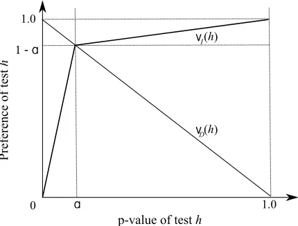
Figure 1: Preference functions νI(h) and νD(h) for statements of independence and dependence

respectively, as functions of the p-value of test h.

the second case (p(X,Y |Z) =1) is reversed—when the value of the statistic is very close to the expected one under independence then independence is preferred. The value of the second case is tempered by the number of variables in the conditioning set. This reflects the practical consideration that, as the number 2+|Z|of variables involved in the test increases, given a fixed data set, the dis-criminatory power of the test diminishes as|Z| →∞. The third case causes the two functionsνIand νDto intersect at p-valueα. This is due to fairness: in the absence of non-propositional arguments

(i.e., in the absence of inference rules in our knowledge base), the independence decisions of the argumentation framework should match those of the purely statistical tests, that is, “dependence” if and only if (p-value≤α). If instead we chose a different intersection point, then the resulting change in the outcome of tests may have been simply due to bias in the independence decision that favors dependence or independence, that is, equivalent to an arbitrary change of the threshold of the statistical test, and the comparison of the statistical and the new test based on argumentation would not be a fair one. The remaining values ofβ are approximated by linear interpolation among the above points. The result is summarized in Fig. 1, which depicts preference functionsνDandνIwith

respect to the p-value of the corresponding statistical test.

Let us illustrate how the preference-based argumentation can be used to resolve the inconsisten-cies of Example 1.

Example 3. In example 1 we considered an IKB with the following propositions

(0⊥⊥1|2) (13)

(06⊥⊥3|2) (14)

(0⊥⊥3| {1,2}) (15)

Following the IKB construction procedure described in the previous section, propositions (13), (14) and (15) correspond to the following arguments, respectively:

n

(0⊥⊥1|2)o,(0⊥⊥1|2)

n

(06⊥⊥3|2)o,(06⊥⊥3|2)

n

(0⊥⊥3| {1,2})o,(0⊥⊥3| {1,2}) (17)

while rule (16) corresponds to the argument

n

(0⊥⊥1|2),(06⊥⊥3|2)o,(06⊥⊥3| {1,2}). (18)

Let us extend this IKB with the following preference values for its propositions and rule.

Pref[(0⊥⊥1|2)] = 0.8

Pref[(06⊥⊥3|2)] = 0.7

Pref[(0⊥⊥3| {1,2})] = 0.5.

According to Definition (12), the preference of each argument({σ},σ)is equal to the preference value of{σ}which is equal to the preference ofσ, as it contains only a single proposition. Thus,

Pref

hn

(0⊥⊥1|2)o,(0⊥⊥1|2)i = 0.8

Prefhn(06⊥⊥3|2)o,(06⊥⊥3|2)i = 0.7

Pref

hn

(0⊥⊥3| {1,2})o,(0⊥⊥3| {1,2})i = 0.5.

The preference of argument (18) equals the preference of the set of its antecedents, which, according to Eq. (12), is equal to the product of their individual preferences, that is,

Pref

hn

(0⊥⊥1|2),(06⊥⊥3|2)o,(06⊥⊥3| {1,2})i = 0.8×0.7=0.56.

Proposition (15) and rule (16) contradict each other logically, that is, their corresponding ar-guments (17) and (18) defeat each other. However, argument (18) is not attacked as its preference is

0.56 which is larger than 0.5, the preference of its defeater argument (17). Since no other argument

defeats (18), it is acceptable, and (17), being attacked by an acceptable argument, must be rejected. We therefore see that using preferences the inconsistency of Example 1 has been resolved in favor of rule (16).

Let us now illustrate the defend relation, that is, how an argument can be defended by some other argument. The example also illustrates an alternative resolution for the inconsistency of Example 1, this time in favor of the independence proposition (15).

Example 4. Let us extend the IKB of Example 3 with two additional independence propositions and

an additional rule. The new propositions and their preference are:

Pref[(0⊥⊥4| {2,3})] = 0.9

and the new rule is:

(0⊥⊥4| {2,3})∧(0⊥⊥3| {2,4}) =⇒ (0⊥⊥3|2).

This rule is an instance of the Intersection axiom followed by Decomposition. The corresponding arguments and preferences are:

Prefhn(0⊥⊥4| {2,3})o,(0⊥⊥4| {2,3})i = 0.9

Pref

hn

(0⊥⊥3| {2,4})o,(0⊥⊥3| {2,4})i = 0.8

corresponding to the two propositions, and

Pref

hn

(0⊥⊥4| {2,3}),(0⊥⊥3| {2,4})o,(0⊥⊥3|2)i =0.9×0.8=0.72 (19)

corresponding to the rule.

As in Example 3, argument (17) is attacked by argument (18). Let us represent this graphically using an arrow from argument a to argument b to denote that a attacks b, that is,

Argument(18)−→Argument(17).

If the IKB was as in Example 3, (18) would had been accepted and (17) would have been rejected. However, the additional argument (19) now defeats (undercuts) (18) by logically contra-dicting its antecedent(06⊥⊥3|2). Since the preference of (19), namely 0.72, is larger than that of

(18), namely 0.56, (19) attacks (18). Therefore, (19) defends all arguments that are attacked by

argument (18), and in particular (17). Graphically,

Argument(19)−→Argument(18)−→Argument(17).

Note this is not sufficient for accepting (17) as it has not been proved that its defender (19) is itself acceptable. We leave the proof of this as an exercise for the reader.

4. The Argumentative Independence Test (AIT)

The independence-based preference argumentation framework described in the previous section provides a semantics for the acceptance of arguments consisting of independence propositions. However, what we need is a procedure for a test of independence that, given as input a triplet

σ= (X,Y |Z) responds whether X is independent or dependent of Y given Z. In other words, we need a semantics for the acceptance of propositions, not arguments. Let us consider the two propositions related to the input triplet σ= (X,Y |Z), proposition (σ=true), abbreviated σt,

and proposition (σ=false), abbreviated σf, that correspond to independence (X⊥⊥Y |Z) and

dependence(X6⊥⊥Y |Z)ofσ, respectively. The basic idea for deciding on the independence or de-pendence of input tripletσis to define a semantics for the acceptance or rejection of propositionsσt

andσfbased on the acceptance or rejection of their respective propositional arguments({σt},σt)

and({σf},σf). Formally,

(X6⊥⊥Y|Z)is accepted iff ({(X6⊥⊥Y|Z)},(X6⊥⊥Y |Z))is accepted, and

Based on this semantics over propositions, we decide on the dependence or independence of tripletσas follows:

σt= (X⊥⊥Y |Z)is accepted =⇒ (X⊥⊥Y |Z)

σf= (X6⊥⊥Y |Z)is accepted =⇒ (X6⊥⊥Y |Z). (21)

We call the test that determines independence in this manner the Argumentative Independence Test or AIT. For the above semantics to be well-defined, a triplet σ must be either independent or dependent, that is, not both or neither. For that, exactly one of the antecedents of the above implications of Eq. (21) must be true. Formally,

Theorem 18. For any input tripletσ= (X,Y |Z), the argumentative independence test (AIT) de-fined by Eqs. (20) and (21) produces a non-ambiguous decision, that is, it decidesσevaluates to either independence or dependence, but nor both or neither.

For that to happen, one and only one of its corresponding propositions σt or σf must be

ac-cepted. A necessary condition for this is given by the following theorem.

Theorem 19. Given a PAFh

A

,

R

,πiwith a strict and transitive preference relationπ, every propo-sitional argument({σt},σt)∈

A

and its negation({σf},σf)satisfy

({σt},σt)is accepted iff({σf},σf)is rejected.

The above theorem is not sufficient because the propositions may still be in abeyance, but this possibility is ruled out for strict preference relations by Theorem 20, presented in the next section.

The formal proofs of Theorems 18, 19 and 20 are presented in Appendix B. We now illustrate the use of AIT with an example.

Example 5. We consider an extension of Example 3 to illustrate the use of the AIT to decide on

the independence or dependence of input triplet(0,3| {1,2}). According to Eq. (20) the decision depends on the status of the two propositional arguments:

({(06⊥⊥3| {1,2})},(06⊥⊥3| {1,2})),and (22)

({(0⊥⊥3| {1,2})},(0⊥⊥3| {1,2})). (23)

Argument (23) is equal to argument (17) of Example 3 that was proved to be rejected in that example. Therefore, according to Theorem 19, its negated propositional argument Eq. (22) must be accepted, and we can conclude that triplet(0,3| {1,2})corresponds to a dependence, that is, we conclude that(06⊥⊥3| {1,2}).

5. The Top-down AIT Algorithm

We now discuss in more detail the top-down algorithm which is used to implement the argumen-tative independence test, introduced in Section 3. We start by simplifying the recursion of Eq. (7) that determines the state (accepted, rejected, or in abeyance) of an argument a. We then explain the algorithm and analyze its computability (i.e., prove that its recursive execution is always finite) and its time complexity.

Theorem 20. Leth

A

,

R

,πibe a PAF with a strict preference relationπ. Then no argument a∈

A

is in abeyance.

This theorem reduces the number of states of each argument to two, that is, an argument can be either accepted or not accepted (rejected). We will use the name of the argument a to denote the predicate “a is accepted” and its negation¬a to denote the predicate “a is rejected.” With this

notation, the above theorem, and the fact that we have extended the semantics of acceptability from the defeat to the attack relation (using preferences), the recursion of Eq. (7) can be expressed as follows

a ⇐⇒ ∀b∈attackers(a),¬b

¬a ⇐⇒ ∃b∈attackers(a),b

or, equivalently,

a ⇐⇒ ^

b∈attackers(a)

¬b

¬a ⇐⇒ _

b∈attackers(a) b.

Finally, we notice that the second formula is logically equivalent to the first (simply negating both sides of the double implication recovers the first). Therefore, the Boolean value of the dialog tree for a can be computed by the simple expression

a ⇐⇒ ^

b∈attackers(a)

¬b. (24)

To illustrate, consider an attacker b of a. If b is rejected, that is,¬b, the conjunction on the right

cannot be determined without examining the other attackers of a. Only when all attackers of a are known to be rejected can the value of a be determined, that is, accepted. Instead, if b is accepted, that is, b, the state of¬b isfalseand the conjunction can be immediately evaluated tofalse, that is, a is rejected regardless of the acceptability of any other attackers.

An iterative version of the top-down algorithm is shown in Algorithm 3. We assume that the algorithm can access a global PAFhA,

R

,πi, with arguments in

A

defined over a knowledge base

K

=hΣ,Ψi. Given as input a triplet t= (X,Y |Z), if the algorithm returnstrue(false) then we conclude that t is independent (dependent). It starts by creating a root node u for the propositional argument U of proposition t=true (lines 1–6). According to Eqs. (20) and (21), the algorithm then decidestrueif U is accepted (line 22). Otherwise, the algorithm returnsfalse(line 23). This is because in this case, according to Theorem 19, the negation of propositional argument U must be accepted.

Algorithm 3 independent(triplet t).

1: ftrue←proposition(t=true) /* Creates independence proposition(t=true). */ 2: Utrue←({ftrue},ftrue)

3: utrue←node for argument Utrue

4: utrue.parent←nil

5: u.STATE←nil

6: f ringe←[u] /* Initialize with u (root). */

7: /* Create global rejected node, denoted byρ. */

8: ρ←node with no argument and staterejected

9: while f ringe6=∅_do

10: u←dequeue(f ringe)

11: attackers←getAttackers(u.argument)

12: if(attackers=∅)_then

13: u.STATE←accepted

14: if sendMsg(ρ,u) =terminate then break

15: attackers←sort attackers in decreasing order of preference.

16: /* Enqueue attackers after decomposing them. */

17: for each A∈attackers do 18: a←node for argument A

19: a.parent←u

20: a.STATE←nil

21: enqueue a in f ringe /* See details in text. */

22: if(u.STATE=accepted)then returntrue

23: if(u.STATE=rejected)then returnfalse

Algorithm 4 sendMsg(Node c,Node p).

1: /* Try to evaluate node p given new information in c.STAT E */ 2: if p6=nilthen

3: if c.STATE=acceptedthen p.STATE←rejected

4: else if (∀children q of p, q.STATE6=rejected) then p.STATE←accepted

5: /* If p was successfully evaluated, try to evaluate its parent by sending message upward. */

6: if p.STATE6=nil then

7: return sendMsg(p,p.parent)

8: else

9: return continue

10: else

11: return terminate /* The root node has been evaluated. */

support H (undercutters), or the negation of its head h (rebutters). Every node maintains a three-valued state variable STATE∈ {nil,accepted,rejected}. Thenilstate denotes that the value of the node is not yet known, and a node is initialized to this state when it is added to the tree.

Algorithm 5 Finds all attackers of input argument a in knowledge base

K

= hΣ,Ψi:

getAttackers(a= (H,h))

1: attackers←∅

2: /* Get all undercutters or rebutters of a. */ 3: for all propositionsϕ∈H∪ {h}do

4: /* Get all defeaters of propositionϕ. */

5: for all rules(Φ1∧Φ2. . .∧Φn =⇒ ¬ϕ)∈Ψ do

6: /* Find all propositionalizations of the rule whose consequent matches¬ϕ. */

7: for all subsets{ϕ1,ϕ2. . . ,ϕn}ofΣs.t. Φ1≡ϕ1,Φ2≡ϕ2. . .Φn≡ϕndo

8: d←({ϕ1∧ϕ2. . .ϕn},¬ϕ)/* Create defeater. */

9: /* Is the defeater an attacker? */

10: if¬(aπd)then

11: attackers←attackers∪ {d}

12: return attackers

time a node receives a message from a child, if the message isaccepted, the node is rejected (line 3 of Algorithm 4), otherwise the node is accepted if all its children has been evaluated torejected (line 4 of Algorithm 4). The subroutine sendMsg then proceeds recursively by forwarding a message to the parent whenever a node has been evaluated (line 7). If the root is reached and evaluated, the message is sent to its parent, which isnil. In this case, the subroutine returns the special keyword

terminate back to the caller, indicating that the root has been evaluated and thus the main algorithm

(Algorithm 3) can terminate. The caller can be either the subroutine sendMsg, in which case it pushes the returned message up the method-calling stack, or the top-down algorithm in line 14, in which case its “while” loop is terminated.

An important part of the algorithm is yet underspecified, namely the order in which the attackers of a node are explored in the tree (i.e., the priority with which nodes are enqueued in line 21). This affects the order of expansion of the nodes in the dialog tree. Possible orderings are depth-first, breadth-first, iterative deepening, as well as informed searches such as best-first when a heuristic is available. In our experiments we used iterative deepening because it combines the benefits of first and breadth-first search, that is, small memory requirements on the same order as depth-first search (i.e., on the order of the maximum number of children a node can have) but also the advantage of finding the shallowest solution like breadth-first search. We also used a heuristic for enqueuing the children of a node. According to iterative deepening, the position in the queue of the children of a node is specified relative to other nodes, but not relative to each other. We therefore specified the relative order of the children according to the value of the preference function: children with higher preference are enqueued first (line 15 of the top-down algorithm), and thus, according to iterative deepening, would be dequeued first.

5.1 Computability of the Top-Down Algorithm

Theorem 21. Given an arbitrary triplet t= (X,Y |Z), and a PAFh

A

,

R

,πiwith a strict preference relationπ, Algorithm 3 with input t overhA,

R

,πiterminates.

The proof consists on showing that the path from the root a to any leaf is always finite. For that, the concept of an attack sequence is needed.

Definition 22. An attack sequence is a sequenceha1,a2, . . . ,aniof n arguments such that for every

2≤i≤n, aiattacks ai−1.

By the manner in which the top-down algorithm constructs the dialog tree it is clear that any path from the root to a leaf is an attack sequence. It therefore suffices to show that any such sequence is finite. This is done by the following theorem.

Theorem 23. Every attack sequenceha1,a2, . . . ,aniin a PAFhA,

R

,πiwith strictπand finite

A

is finite.

Intuitively, if the preference relation is strict then an element can attack its predecessor in the sequence but not vice versa. Since the set of arguments

A

is finite, the only way for an attack sequence to be infinite is to contain a cycle. In that case, an argument would be attacking at least one of its predecessors, which cannot happen in a PAF with a strict preference relation. We present formal proofs of Theorems 21 and 23 in Appendix A.

We thus arrived at the important conclusion that, under a strict preference function and a finite argument set, the state of any argument is computable. As we showed in Section 3.3, the preference function for independence knowledge bases is strict, and thus the computability of the top-down algorithm is guaranteed.

5.2 Computational Complexity of the Top-Down Algorithm

Since Algorithm 3 is a tree traversal algorithm, its time complexity can be obtained by techniques contained in standard algorithmic texts, for example, Cormen et al. (2001). The actual performance depends on the tree exploration procedure. In our case we used iterative deepening due to its linear memory requirements in d, where d is the smallest depth at which the algorithm terminates. Iterative deepening has a worst-time time complexity of O(bd), where b is an upper bound on the dialog tree

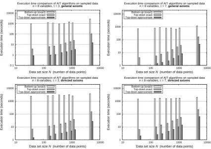
branching factor. Therefore, for a constant b>1 the execution time is exponential in d in the worst case. Furthermore, for the case of independence tests, b itself may also be exponential in n (the number of variables in the domain). This is because the inference rules of Eqs. (5) and (6) are universally quantified, and therefore their propositionalization (lines 7–11 of Algorithm 5), may result in an exponential number of rules with the same consequent (attackers). A tighter bound may be possible but, lacking such a bound, we introduce in the next section an approximate top-down algorithm, which reduces the running time to polynomial. As we show in our experiments, the use of this approximation does not appreciably affect the accuracy improvement due to argumentation.

6. The Approximate Top-Down AIT Algorithm

exponential size of the branching factor b (which equals the maximum number of defeaters of any argument appearing in the dialog tree) we limit the number of defeaters of each node—thus bounding the number of its attackers/children—to a polynomial function of n (the domain size) during the propositionalization process of Algorithm 5 (lines 7–11). Let(H,h)be an argument and letϕ∈H∪ {h}be one of its propositions, as in line 3 of Algorithm 5. The set of attackersΣϕof (H,h)consists of all rules{ϕ1∧ϕ2. . .∧ϕk =⇒ ¬ϕ}ofΣ, for some constant upper bound k on the

size of their support. Ifϕ= (X,Y|Z)andϕi= (Xi,Yi|Zi)for all 1≤i≤k, then our approximation

generates and uses a subset ofΣϕin the dialog tree such that

|X| −c ≤ |Xi| ≤ |X|+c

|Y| −c ≤ |Yi| ≤ |Y|+c (25)

|Z| −c ≤ |Zi| ≤ |Z|+c

where| · |denotes set cardinality, and c is a user-specified integer parameter that defines the approx-imation. We call this the approximate top-down algorithm. The computational complexity of the approximate top-down algorithm is polynomial in n, as shown in the next section.

6.1 Test Complexity of the Approximate Top-Down Algorithm

In this section we prove that the number of statistical tests required by the Approximate Top-Down algorithm is polynomial in n. As described in the previous section, the approximate algorithm generates a bounded number of attackers for each proposition in the argument corresponding to some node in the dialog tree. A bound on the number of the possible attackers can be defined by the approximation of Eq. (25). These equations dictate that the size of each possible set Xi in some

proposition(Xi,Yi|Zi)of some attacker of proposition(X,Y|Z) is between|X|+c and|X| −c

(inclusively). As the number of elements that can be members of Xi is bounded by n (the domain

size), this produces at most n2c+1possible instantiations for set Xi. Similarly, the number of possible

instantiations for Yi and Zi is also n2c+1. Therefore, an upper bound for the number of matches to

some proposition in the antecedent of an attacking rule is O(n6c+3)for some constant c. As there are

r rules in the rule set and up to k propositions in each rule for some constants r and k (for example, r=5 and k=3 for Eq. (5) and r=8 and k=4 for Eq. (6)), an upper bound on the number of children of a node in the dialog tree is O(rkn6c+3), and thus an upper bound on the number of nodes in the dialog tree of depth d is O((rk)d_nd(6c+3)_{). As we demonstrate in our experiments, this is a}

rather loose upper bound and the performance of the approximate top-down algorithm is reasonable in practice, but it does serve to show that the theoretical worst-case performance is polynomial in n. In the experiments shown in the next section we used c=1 and d=3.

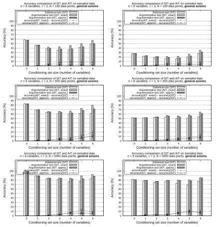
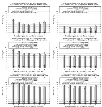
7. Experimental Results