Hash Kernels for Structured Data
Qinfeng Shi [email protected]
College of Engineering and Computer Science The Australian National University
Canberra, ACT 0200, Australia
James Petterson [email protected]
Statistical Machine Learning National ICT Australia Locked Bag 8001
Canberra, ACT 2601, Australia
Gideon Dror [email protected]
Division of Computer Science
Academic College of Tel-Aviv-Yaffo, Israel
John Langford [email protected]
Alex Smola [email protected]
Yahoo! Research
New York, NY and Santa Clara, CA, USA
S.V.N. Vishwanathan [email protected]
Department of Statistics Purdue University, IN, USA
Editor: Soeren Sonnenburg, Vojtech Franc, Elad Yom-Tov and Michele Sebag
Abstract
We propose hashing to facilitate efficient kernels. This generalizes previous work using sampling and we show a principled way to compute the kernel matrix for data streams and sparse feature spaces. Moreover, we give deviation bounds from the exact kernel matrix. This has applications to estimation on strings and graphs.
Keywords: hashing, stream, string kernel, graphlet kernel, multiclass classification
1. Introduction
In recent years, a number of methods have been proposed to deal with the fact that kernel methods have slow runtime performance if the number of kernel functions used in the expansion is large. We denote byXthe domain of observations and we assume thatHis a Reproducing Kernel Hilbert SpaceHwith kernel k :X×X→R.
1.1 Keeping the Kernel Expansion Small
b) use a subset of basis functions to approximate the exact solution, c) use the latter for estimation. While the approximation of the full function expansion is typically not very accurate, very good generalization performance is reported. The big problem in this approach is that the optimization of the reduced set of vectors is rather nontrivial.
Work on estimation on a budget (Dekel et al., 2006) tries to ensure that this problem does not arise in the first place by ensuring that the number of kernel functions used in the expansion never exceeds a given budget or by using anℓ1 penalty (Mangasarian, 1998). For some algorithms, for example, binary classification, guarantees are available in the online setting.
1.2 Keeping the Kernel Simple
A second line of research uses variants of sampling to achieve a similar goal. That is, one uses the feature map representation
k(x,x′) =
φ(x),φ(x′)
.
HereφmapsXinto some feature spaceF. This expansion is approximated by a mappingφ:X→F
k(x,x′) =φ(
x),φ(x′)
oftenφ(x) =Mφ(x).
Hereφhas more desirable computational properties than φ. For instance, φis finite dimensional (Fine and Scheinberg, 2001; Kontorovich, 2007; Rahimi and Recht, 2008), orφis particularly sparse (Li et al., 2007).
1.3 Our Contribution
Firstly, we show that the sampling schemes of Kontorovich (2007) and Rahimi and Recht (2008) can be applied to a considerably larger class of kernels than originally suggested—the authors only consider languages and radial basis functions respectively. Secondly, we propose a biased approxi-mationφofφwhich allows efficient computations even on data streams. Our work is inspired by the count-min sketch of Cormode and Muthukrishnan (2004), which uses hash functions as a computa-tionally efficient means of randomization. This affords storage efficiency (we need not store random vectors) and at the same time they give performance guarantees comparable to those obtained by means of random projections.
As an application, we demonstrate computational benefits over suffix array string kernels in the case of document analysis and we discuss a kernel between graphs which only becomes computa-tionally feasible by means of compressed representation.
1.4 Outline
2. Previous Work and Applications
Recently much attention has been paid to efficient algorithms with randomization or hashing in the machine learning community.
2.1 Generic Randomization
Kontorovich (2007) and Rahimi and Recht (2008) independently propose the following: denote by c∈Ca random variable with measure P. Moreover, letφc:X→Rbe functions indexed by c∈C. For kernels of type
k(x,x′) =Ec∼P(c)
φc(x)φc(x′)
(1)
an approximation can be obtained by sampling C={c1, . . . ,cn} ∼P and expanding
k(x,x′) =1
n
n
∑
i=1
φci(x)φci(x′).
In other words, we approximate the feature map φ(x) by φ(x) = n−12(φc
1(x), . . . ,φcn(x)) in the
sense that their resulting kernel is similar. Assuming that φc(x)φc(x′)has bounded range, that is, φc(x)φc(x′)∈[a,a+R]for all c, x and x′one may use Chernoff bounds to give guarantees for large deviations between k(x,x′) and k(x,x′). For matrices of size m×m one obtains bounds of type O(R2ε−2log m) by combining Hoeffding’s theorem with a union bound argument over the O(m2)
different elements of the kernel matrix. The strategy has widespread applications beyond those of Kontorovich (2007) and Rahimi and Recht (2008):
• Kontorovich (2007) uses it to design kernels on regular languages by sampling from the class of languages.
• The marginalized kernels of Tsuda et al. (2002) use a setting identical to (1) as the basis for comparisons between strings and graphs by defining a random walk as the feature extractor. Instead of exact computation we could do sampling.
• The Binet-Cauchy kernels of Vishwanathan et al. (2007b) use this approach to compare tra-jectories of dynamical systems. Here c is the (discrete or continuous) time and P(c)discounts over future events.
• The empirical kernel map of Sch¨olkopf (1997) usesC=Xand employs some kernel function
κto defineφc(x) =κ(c,x). Moreover, P(c) =P(x), that is, placing our sampling points ci on training data.
• For RBF kernels, Rahimi and Recht (2008) use the fact that k may be expressed in the system of eigenfunctions which commute with the translation operator, that is the Fourier basis
k(x,x′) =Ew∼P(w)[e−ihw,xieihw,x
′i
]. (2)
Here P(w)is a nonnegative measure which exists for any RBF kernel by virtue of Bochner’s theorem, hence (2) can be recast as a special case of (1). What sets it apart is the fact that the variance of the featuresφw(x) =eihw,xiis relatively evenly spread. (2) extends immediately to Fourier transformations on other symmetry groups (Berg et al., 1984).
While in many cases straightforward sampling may suffice, it can prove disastrous wheneverφc(x) has only a small number of significant terms. For instance, for the pair-HMM kernel most strings c are unlikely ancestors of x and x′, hence P(x|c)and P(x′|c) will be negligible for most c. As a consequence the number of strings required to obtain a good estimate is prohibitively large—we need to reduceφfurther.
2.2 Locally Sensitive Hashing
The basic idea of randomized projections (Indyk and Motawani, 1998) is that due to concentration of measures the inner producthφ(x),φ(x′)ican be approximated by∑ni=1hvi,φ(x)ihvi,φ(x′)iefficiently, provided that the distribution generating the vectors vi satisfies basic regularity conditions. For example, vi∼N(0,I)is sufficient, where I is an identity matrix. This allows one to obtain Chernoff bounds and O(ε−2log m)rates of approximation, where m is the number of instances. The main cost is to store viand perform the O(nm)multiply-adds, thus rendering this approach too expensive as a preprocessing step in many applications.
Achlioptas (2003) proposes a random projection approach that uses symmetric random variables to project the original feature onto a lower dimension feature space. This operation is simple and faster and the author shows it does not sacrifice the quality of the embedding. Moreover, it can be directly applied to online learning tasks. Unfortunately, the projection remains dense resulting in relatively poor computational and space performance in our experiments.
2.3 Sparsification
Li et al. (2007) propose to sparsifyφ(x)by randomization while retaining the inner products. One problem with this approach is that when performing optimization for linear function classes, the weight vector w which is a linear combination ofφ(xi)remains large and dense, thus obliterating a significant part of the computational savings gained in sparsifyingφ.
2.4 Count-Min Sketch
Cormode and Muthukrishnan (2004) propose an ingenious method for representing data streams. Denote byIan index set. Moreover, let h :I→ {1, . . . ,n}be a hash function and assume that there exists a distribution over h such that they are pairwise independent.
Assume that we draw d hash functions hi at random and let S∈Rn×d be a sketch matrix. For a stream of symbols s update Shi(s),i←Shi(s),i+1 for all 1≤i≤d. To retrieve the (approximate)
counts for symbol s′ compute miniShi(s′),i. Hence the name count-min sketch. The idea is that
by storing counts of s according to several hash functions we can reduce the probability of colli-sion with another particularly large symbol. Cormode and Muthukrishnan (2004) show that only O(ε−1log 1/δ)storage is required for anε-good approximation, where 1−δis the confidence.
2.5 Random Feature Mixing
Ganchev and Dredze (2008) provide empirical evidence that using hashing can eliminate alphabet storage and reduce the number of parameters without severely impacting model performance. In addition, Langford et al. (2007) released the Vowpal Wabbit fast online learning software which uses a hash representation similar to the one discussed here.
2.6 Hash Kernel on Strings
Shi et al. (2009) propose a hash kernel to deal with the issue of computational efficiency by a very simple algorithm: high-dimensional vectors are compressed by adding up all coordinates which have the same hash value—one only needs to perform as many calculations as there are nonzero terms in the vector. The hash kernel can jointly hash both label and features, thus the memory footprint is essentially independent of the number of classes used.
3. Hash Kernels
Our goal is to design a possibly biased approximation which a) approximately preserves the inner product, b) which is generally applicable, c) which can work on data streams, and d) which increases the density of the feature matrices (the latter matters for fast linear algebra on CPUs and graphics cards).
3.1 Kernel Approximation
As before denote by I an index set and let h :I→ {1, . . . ,n} be a hash function drawn from a distribution of pairwise independent hash functions. Finally, assume thatφ(x)is indexed byIand that we may computeφi(x)for all nonzero terms efficiently. In this case we define the hash kernel as follows:
k(x,x′) =
φ(x),φ(x′)
withφj(x) =
∑
i∈I;h(i)=jφi(x) (3)
We are accumulating all coordinates i ofφ(x)for which h(i)generates the same value j into coordi-nateφj(x). Our claim is that hashing preserves information as well as randomized projections with significantly less computation. Before providing an analysis let us discuss two key applications: efficient hashing of kernels on strings and cases where the number of classes is very high, such as categorization in an ontology.
3.2 Strings
Denote byX=Ithe domain of strings on some alphabet. Moreover, assume thatφi(x):=λi#i(x) denotes the number of times the substring i occurs in x, weighted by some coefficientλi≥0. This allows us to compute a large family of kernels via
k(x,x′) =
∑
i∈Iλ2
i#i(x)#i(x′). (4)
The big drawback with string kernels using suffix arrays/trees is that they require large amounts of working memory. Approximately a factor of 50 additional storage is required for processing and analysis. Moreover, updates to a weighted combination are costly. This makes it virtually impossible to apply (4) to millions of documents. Even for modest document lengths this would require Terabytes of RAM.
Hashing allows us to reduce the dimensionality. Since for every document x only a relatively small number of terms #i(x) will have nonzero values—at most O(|x|2) but in practice we will restrict ourselves to substrings of a bounded length l leading to a cost of O(|x| ·l)—this can be done efficiently in a single pass over x. Moreover, we can computeφ(x) as a pre-processing step and discard x altogether.
Note that this process spreads out the features available in a document evenly over the coordi-nates ofφ(x). Moreover, note that a similar procedure can be used to obtain good estimates for a TF/IDF reweighting of the counts obtained, thus rendering preprocessing as memory efficient as the actual computation of the kernel.
3.3 Multiclass
Classification can sometimes lead to a very high dimensional feature vector even if the underly-ing feature map x→φ(x)may be acceptable. For instance, for a bag-of-words representation of documents with 104 unique words and 103 classes this involves up to 107 coefficients to store the parameter vector directly when theφ(x,y) =ey⊗φ(x), where⊗is the tensor product and ey is a vector whose y-th entry is 1 and the rest are zero. The dimensionality of eyis the number of classes. Note that in the above caseφ(x,y)corresponds to a sparse vector which has nonzero terms only in the part corresponding to ey. That is, by using the joint index(i,y)withφ(x,y)(i,y′)=φi(x)δy,y′
we may simply apply (3) to an extended index to obtain hashed versions of multiclass vectors. We have
φj(x,y) =
∑
i∈I;h(i,y)=jφi(x).
In some cases it may be desirable to compute a compressed version ofφ(x), that is,φ(x)first and subsequently expand terms with y. In particular for strings this can be useful since it means that we need not parse x for every potential value of y. While this deteriorates the approximation in an additive fashion it can offer significant computational savings since all we need to do is permute a given feature vector as opposed to performing any summations.
3.4 Streams
Some features of observations arrive as a stream. For instance, when performing estimation on graphs, we may obtain properties of the graph by using an MCMC sampler. The advantage is that we need not store the entire data stream but rather just use summary statistics obtained by hashing.
4. Analysis
unable to obtain the excellent O(ε−1)rates offered by the count-min sketch, our approach retains the inner product property thus making hashing accessible to linear estimation.
4.1 Bias and Variance
A first step in our analysis is to compute bias and variance of the approximation φ(x) of φ(x). Whenever needed we will writeφh(x)and kh(x,x′)to make the dependence on the hash function h explicit. Using (3) we have
kh(x,x′) =
∑
j i:h∑
(i)=jφi(x)
∑
i′:h(i′)=jφ′ i(x′)
=k(x,x′) +
∑
i,i′:i6=i′φi(x)φi′(x′)δh(i),h(i′) (5)
whereδis the Kronecker delta function. Taking the expectation with respect to the random choice of hash functions h we obtain the expected bias
Eh[k h
(x,x′)] = 1−1n
k(x,x′) +1
n
∑
iφi(x)
∑
i′φi′(x′)
Here we exploited the fact that for a random choice of hash functions the collision probability is 1n uniformly over all pairs(i,j). Consequently k(x,x′)is a biased estimator of the kernel matrix, with the bias decreasing inversely proportional to the number of hash bins.
The main change is a rank-1 modification in the kernel matrix. Given the inherent high dimen-sionality of the estimation problem, a one dimensional change does not in general have a significant effect on generalization.
Straightforward (and tedious) calculation which is completely analogous to the above derivation leads to the following expression for the variance Varh[k
h
(x,x′)]of the hash kernel:
Varh[k h
(x,x′)] = nn−21
k(x,x)k(x′,x′) +k2(x,x′)−2
∑
iφ2
i(x)φ2i(x′)
Key in the derivation is our assumption that the family of hash functions we are dealing with is pairwise independent.
As can be seen, the variance decreases O(n−1)in the size of the values of the hash function. This means that we have an O(n−12)convergence asymptotically to the expected value of the kernel.
4.2 Information Loss
One of the key fears of using hashing in machine learning is that hash collisions harm performance. For example, the well-known birthday paradox shows that if the hash function maps into a space of size n then with O(n12) features a collision is likely. When a collision occurs, information is lost,
which may reduce the achievable performance for a predictor.
Definition 1 (Information Loss) A hash function h causes information loss on a distribution D with a loss function L if the expected minimum loss before hashing is less than the expected minimum loss after hashing:
min f (x,yE)∼D
[L(f(x),y))]<min
Redundancy in features is very helpful in avoiding information loss. The redundancy can be explicit or systemic such as might be expected with a bag-of-words or substring representation. In the following we analyze explicit redundancy where a feature is mapped to two or more values in the space of size n. This can be implemented with a hash function by (for example) appending the string i∈ {1, . . . ,c}to feature f and then computing the hash of f◦i for the i-th duplicate.
The essential observation is that the information in a feature is only lost if all duplicates of the feature collide with other features. Given this observation, it’s unsurprising that increasing the size of n by a constant multiple c and duplicating features c times makes collisions with all features unlikely. It’s perhaps more surprising that when keeping the size of n constant and duplicating features, the probability of information loss can go down.
Theorem 2 For a random function mapping l features duplicated c times into a space of size n, for all loss functions L and and distributions D on n features, the probability (over the random function) of no information loss is at least:
1−l[1−(1−c/n)c+ (lc/n)c].
To see the implications consider l=105 and n=108. Without duplication, a birthday paradox collision is virtually certain. However, if c=2, the probability of information loss is bounded by about 0.404, and for c=3 it drops to about 0.0117.
Proof The proof is essentially a counting argument with consideration of the fact that we are dealing with a hash function rather than a random variable. It is structurally similar to the proof for a Bloom filter (Bloom, 1970), because the essential question we address is: “What is a lower bound on the probability that all features have one duplicate not colliding with any other feature?”
Fix a feature f . We’ll argue about the probability that all c duplicates of f collide with other features.
For feature duplicate i, let hi=h(f◦i). The probability that hi=h(f′◦i′)for some other feature
f′◦i′is bounded by(l−1)c/n because the probability for each other mapping of a collision is 1/n by the assumption that h is a random function, and the union bound applied to the(l−1)c mappings of other features yields(l−1)c/n. Note that we do not care about a collision of two duplicates of the same feature, because the feature value is preserved.
The probability that all duplicates 1≤i≤c collide with another feature is bounded by(lc/n)c+ 1−(1−c/n)c. To see this, let c′≤c be the number of distinct duplicates of f after collisions. The probability of a collision with the first of these is bounded by (l−n1)c. Conditioned on this collision, the probability of the next collision is at most (l−n1)−c1−1, where 1 is subtracted because the first location is fixed. Similarly, for the ith duplicate, the probability is(l−n1)−c(−i−(1)i−1). We can upper bound each term as lcn, implying the probability of all c′duplicates colliding with other features is at most
(lc/n)c′. The probability that c′=c is the probability that none of the duplicates of f collide, which is nc((nn−−c1)!−1)! ≥((n−c)/n)c. If we pessimistically assume that c′<c implies that every duplicate
collides with another feature, then
P(coll)≤P(coll|c′=c)P(c′=c) +P(c′6=c)
≤(lc/n)c+1−((l−c)/l)c.
(lc/n)c].
4.3 Rate of Convergence
As a first step note that any convergence bound only depends logarithmically on the size of the kernel matrix.
Theorem 3 Assume that the probability of deviation between the hash kernel and its expected value is bounded by an exponential inequality via
P h
k
h
(x,x′)−Eh h
kh(x,x′)i >ε
i
≤c exp(−c′ε2n)
for some constants c,c′depending on the size of the hash and the kernel used. In this case the error
εarising from ensuring the above inequality, with probability at least 1−δ, for m observations and M classes (for a joint feature mapφ(x,y), is bounded by
ε≤p
(2 log(m+1) +2 log(M+1)−logδ+log c−2 log 2)/nc′.
Proof Apply the union bound to the kernel matrix of size(mM)2, that is, to all T :=m(m+1)M(M+ 1)/4 unique elements. Solving
T c exp(−c′ε2n) =δ,
we get the bound onεis
r
log(T c)−logδ
c′n . (6)
Bounding log(T c)from above
log(T c) =log T+log c≤2 log(m+1) +2 log(M+1) +log c−2 log 2,
and plugging it into (6) yields the result.
4.4 Generalization Bound
The hash kernel approximates the original kernel by big storage and computation saving. An inter-esting question is whether the generalization bound on the hash kernel will be much worse than the bound obtained on the original kernel.
Theorem 4 (Generalization Bound) For binary class SVM, let K=φ(
x),φ(x′)
,K=hφ(x),φ(x′)i
be the hash kernel matrix and original kernel matrix. Assume there exists b≥0 such that b≥
δ∈(0,1)and anyγ>0, with probability at least 1−δ, we have
P(y6=sgn(g(x)))≤ 1
mγ
m
∑
i=1
ξi+ 4 mγ
q
tr(K) +3 s
ln(2δ)
2m (7)
≤ m1γ
m
∑
i=1
ξi+ 4 mγ
p
tr(K) + 4
mγ √
b+3 s
ln(2
δ)
2m , (8)
whereξi=max{0,γ−yig(xi)}, and g(xi) =
w,φ(xi,yi)
.
Proof The standard Rademacher bound states that for any size m sample drawn i.i.d from D, for anyδ∈(0,1)and anyγ>0, with probability at least 1−δ, the true error of the binary SVM ,whose kernel matrix is denoted as K′, can be bounded as follows:
P(y6=sgn(g(x)))≤ 1
mγ
m
∑
i=1
ξi+ 4 mγ
p
tr(K′) +3 s
ln(2
δ)
2m . (9)
We refer the reader to Theorem 4.17 in Shawe-Taylor and Cristianini (2004) for a detailed proof. The inequality (7) follows by letting K′ =K. Because tr(K)≤b+tr(K)≤(√b+ptr(K))2, we have m4γptr(K)≤ 4
mγ p
tr(K) + 4
mγ
√
b. Plugging above inequality into inequality (7) gives inequal-ity (8). So the theorem holds.
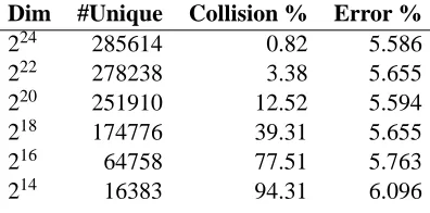
The approximation quality depends on the both the feature and the hash collision. From the defini-tion of hash kernel (see (3)), the feature entries with the same hash value will add up and map to a new feature entry indexed by the hash value. The higher collision of the hash has, the more entries will be added up. If the feature is sparse, the added up entries are mostly zeros. So the difference of the maximum and the sum of the entries is reasonably small. In this case, the hash kernel gives a good approximation of the original kernel, so b is reasonably small. Thus the generalization error does not increase much as the collision increases. This is verified in the experiment section in Ta-ble 4—increasing the collision rate from 0.82% to 94.31% only slightly worsens the test error (from 5.586% to 6.096%).
Moreover, Theorem 4 shows us the generalization bounds on the hash kernel and the original kernel only differ by O((mγ)−1). This means that when our data set is large, the difference can be ignored. A surprising result as we shall see immediately is that in fact, the difference on the generalization bound is always nearly zero regardless of m,γ.
4.5 The Scaling Factor Effect
An interesting observation on Theorem 4 is that, if we use a new feature mappingφ′=aφ, where a∈[0,1), it will make the bias term in (5) small. As we decrease a enough, the bias term can be arbitrarily small. Indeed, it vanishes when a=0. It seems that thus we can get a much tighter bound according to Theorem 4—the term with b vanishes when a=0. So is there an optimal scaling factor a that maximizes the performance? It turns out that any nonzero a doesn’t effect the performance at all, although it does tighten the bound.
Let’s take a closer look at the hash kernel binary SVM, which can be formalized as
min w
λ||w||2
2 +
m
∑
i=1
max{0,1−yi
w,φ(xi,yi)
Applying a new feature mapping ˆφ=aφgives
min ˆ
w ˆ
λ||wˆ||2
2 +
m
∑
i=1
max{0,1−yi
ˆ
w,φ(xi,yi)
}, (11)
where ˆλ= aλ2 and ˆw=aw. ˆλ is usually determined by model selection. As we can see, given a
training data set, the solutions to (10) and (11) are exactly identical for a6=0. When a=0, g(x)≡0 for all x,w, and the prediction degenerates to random guessing. Moreover, the generalization bound can be tighten by applying a small a nearly zero. This shows that hashing kernel SVM has nearly the same generalization bound as the original SVM in theory.
5. Graphlet Kernels
Denote by G a graph with vertices V(G)and edges E(G). Several methods have been proposed to perform classification on such graphs. Most recently, Przulj (2007) proposed to use the distribution over graphlets, that is, subgraphs, as a characteristic property of the graph. Unfortunately, brute force evaluation does not allow calculation of the statistics for graphlets of size more than 5, since the cost for exact computation scales exponentially in the graphlet size.
In the following we show that sampling and hashing can be used to make the analysis of larger subgraphs tractable in practice. For this denote by S⊆G an induced subgraph of G, obtained by restricting ourselves to only V(S)⊆V(G) vertices of G and let #S(G) be the number of times S occurs in G. This suggests that the feature map G→φ(G), where φS(G) =#S(G)will induce a useful kernel: adding or removing an edge(i,j)only changes the properties of the subgraphs using the pair(i,j)as part of their vertices.
5.1 Counting and Sampling
Depending on the application, the distribution over the counts of subgraphs may be significantly skewed. For instance, in sparse graphs we expect the fully disconnected subgraphs to be con-siderably overrepresented. Likewise, whenever we are dealing with almost complete graphs, the distribution may be skewed towards the other end (i.e., most subgraphs will be complete). To deal with this, we impose weightsβ(k)on subgraphs containing k edges|E(S)|.
To deal with the computational complexity issue simultaneously with the issue of reweighting the graphs S we simply replace explicit counting with sampling from the distribution
P(S|G) =c(G)β(|E(S)|) (12)
where c(G)is a normalization constant. Samples from P(S|G)can be obtained by a Markov-Chain Monte Carlo approach.
Lemma 5 The following MCMC sampling procedure has the stationary distribution (12).
1. Choose a random vertex, say i, of S uniformly.
2. Add a vertex j from G\Sito Si with probability c(Si,G)β(|E(Si j)|).
Here Si denotes the subgraph obtained by removing vertex i from S, and Si j is the result of adding
Note that sampling over j is easy: all vertices of G which do not share an edge with S\i occur with the same probability. All others depend only on the number of joining edges. This allows for easy computation of the normalization c(Si,G).
Proof We may encode the sampling rule via
T(Si j|S,G) = 1
kc(Si,G)β(|E(Si j)|)
where c(Si,G) is a suitable normalization constant. Next we show that T satisfies the balance equations and therefore can be used as a proposal distribution with acceptance probability 1.
T(Si j|S,G)P(S)
T(S|Si j,G)P(Si j)
= k−
1c(S
i,G)β(|E(Si j)|)c(G)β(|E(S)|)
k−1c(S
i j,j,G)β(|E(Si j,ji)|)c(G)β(|E(Si j)|) =1.
This follows since Si j,j =Siand likewise Si j,ji=S. That is, adding and removing the same vertex leaves a graph unchanged.
In summary, we obtain an algorithm which will readily draw samples S from P(S|G)to characterize G.
5.2 Dependent Random Variables
The problem with sampling from a MCMC procedure is that the random variables are dependent on each other. This means that we cannot simply appeal to Chernoff bounds when it comes to averaging. Before discussing hashing we briefly discuss averages of dependent random variables:
Definition 6 (Bernoulli Mixing) Denote by Z a stochastic process indexed by t∈Zwith probabil-ity measure P and letΣnbe theσ-algebra on Zt with t ∈Z\1, . . . ,n−1. Moreover, denote by P− and P+ the probability measures on the negative and positive indices t respectively. The mixing coefficientβis
β(n,PX):= sup A∈Σn
P(A)−P−×P+(A) .
If limn→∞β(n,Pz) =0 we call Z to beβ-mixing.
That is, β(n,PX) measures how much dependence a sequence has when cutting out a segment of length n. Nobel and Dembo (1993) show how such mixing processes can be related to iid observa-tions.
Theorem 7 Assume that P is β-mixing. Denote by P∗ the product measure obtained from . . .Pt×Pt+1. . .Moreover, denote byΣl,ntheσ-algebra on Zn,Z2n, . . . ,Zln. Then the following holds:
sup A∈Σl,n
|P(A)−P∗(A)| ≤lβ(n,P).
Theorem 8 Let P be a distribution over a domainXand denote byφ:X→Ha feature map into a Hilbert Space withhφ(x),φ(x′)i ∈[0,1]. Moreover, assume that there is aβ-mixing MCMC sampler of P with distribution PMCfrom which we draw l observations xin with an interleave of n rather
than sampling from P directly. Averages with respect to PMCsatisfy the following with probability at least 1−δ:
E
x∼P([φ(x)x)]− 1 l
l
∑
i=1
φ(xin)
≤lβ(n,P
MC) +2+
q log2δ √
l .
Proof Theorem 7, the bound onkφ(x)k, and the triangle inequality imply that the expectations with respect to PMC and P∗ only differ by lβ. This establishes the first term of the bound. The second term is given by a uniform convergence result in Hilbert Spaces from Altun and Smola (2006).
Hence, sampling from a MCMC sampler for the purpose of approximating inner products is sound, provided that we only take sufficiently independent samples (i.e., a large enough n) into account. The translation of Theorem 8 into bounds on inner products is straightforward, since
|hx,yi −x′,y′| ≤x−x′
kyk+
y−y′
kxk+
x−x′
y−y′
.
5.3 Hashing and Subgraph Isomorphism
Sampling from the distribution over subgraphs S∈G has two serious problems in practice which we will address in the following: firstly, there are several graphs which are isomorphic to each other. This needs to be addressed with a graph isomorphism tester, such as Nauty (McKay, 1984). For graphs up to size 12 this is a very effective method. Nauty works by constructing a lookup table to match isomorphic objects.
However, even after the graph isomorphism mapping we are still left with a sizable number of distinct objects. This is where a hash map on data streams comes in handy. It obviates the need to store any intermediate results, such as the graphs S or their unique representations obtained from Nauty. Finally, we combine the convergence bounds from Theorem 8 with the guarantees available for hash kernels to obtain the approximate graph kernel.
Note that the two randomizations have very different purposes: the sampling over graphlets is done as a way to approximate the extraction of features whereas the compression via hashing is carried out to ensure that the representation is computationally efficient.
6. Experiments
To test the efficacy of our approach we applied hashing to the following problems: first we used it for classification on the Reuters RCV1 data set as it has a relatively large feature dimensionality. Secondly, we applied it to the DMOZ ontology of topics of webpages1where the number of topics is high. The third experiment—Biochemistry and Bioinformatics Graph Classification uses our hashing scheme, which makes comparing all possible subgraph pairs tractable, to compare graphs (Vishwanathan et al., 2007a). On publicly available data sets like MUTAG and PTC as well as on
Data Sets #Train #Test #Labels
RCV1 781,265 23,149 2
Dmoz L2 4,466,703 138,146 575 Dmoz L3 4,460,273 137,924 7,100
Table 1: Text data sets. #X denotes the number of observations in X.
Algorithm Pre TrainTest Error %
BSGD 303.60s 10.38s 6.02
VW 303.60s 87.63s 5.39
VWC 303.60s 5.15s 5.39
HK 0s 25.16s 5.60
Table 2: Runtime and Error on RCV1. BSGD: Bottou’s SGD. VW: Vowpal Wabbit without cache. VWC: Vowpal Wabbit using cache file. HK: hash kernel with feature dimension 220. Pre: prepro-cessing time. TrainTest: time to load data, train and test the model. Error: misclassification rate. Apart from the efficacy of hashing operation itself, the gain of speed is also due to a multi-core implementation—hash kernel uses 4-cores to access the disc for online hash feature generation. For learning and testing evaluation, all algorithms use single-core.
the biologically inspired data set DD used by Vishwanathan et al. (2007a), our method achieves the best known accuracy.
In both RCV1 and Dmoz, we use linear kernel SVM with stochastic gradient descent (SGD) as the workhorse. We apply our hash kernels and random projection (Achlioptas, 2003) to the SGD linear SVM. We don’t apply the approach in Rahimi and Recht (2008) since it requires a shift-invariant kernel k(x,y) =k(x−y), such as RBF kernel, which is not applicable in this case. In the third experiment, existing randomization approaches are not applicable since enumerating all possible subgraphs is intractable. Instead we compare hash kernel with existing graph kernels: random walk kernel, shortest path kernel and graphlet kernel (see Borgwardt et al. 2007).
6.1 Reuters Articles Categorization
We use the Reuters RCV1 binary classification data set (Lewis et al., 2004). 781,265 articles are used for training by stochastic gradient descent (SGD) and 23,149 articles are used for testing. Con-ventionally one would build a bag of words representation first and calculate exact term frequency / inverse document frequency (TF-IDF) counts from the contents of each article as features. The problem is that the TF calculation needs to maintain a very large dictionary throughout the whole process. Moreover, it is impossible to extract features online since the entire vocabulary dictionary is usually unobserved during training. Another disadvantage is that calculating exact IDF requires us to preprocess all articles in a first pass. This is not possible as articles such as news may vary daily.
Algorithm Dim Pre TrainTest orgTrainSize newTrainSize Error %
28 748.30s 210.23s 423.29Mb 1393.65Mb 29.35%
RP 29 1079.30s 393.46s 423.29Mb 2862.90Mb 25.08%
210 1717.30s 860.95s 423.29Mb 5858.48Mb 19.86%
28 0s 22.82s NA NA 17.00%
HK 29 0s 24.19s NA NA 12.32%
210 0s 24.41s NA NA 9.93%
Table 3: Hash kernel vs. random projections with various feature dimensionalities on RCV1. RP: random projections in Achlioptas (2003). HK: hash kernel. Dim: dimension of the new features. Pre: preprocessing time. TrainTest: time to load data, train and test the model. orgTrainSize: compressed original training feature file size. newTrainSize: compressed new training feature file size. Error: misclassification rate. NA: not applicable. In hash kernel there is no preprocess step, so there is no original/new feature files. Features for hash kernel are built up online via accessing the string on disc. The disc access time is taken into account in TrainTest. Note that the TrainTest for random projection time increases as the new feature dimension increases, whereas for hash kernel the TrainTest is almost independent of the feature dimensionality.
Dim #Unique Collision % Error %
224 285614 0.82 5.586
222 278238 3.38 5.655
220 251910 12.52 5.594
218 174776 39.31 5.655
216 64758 77.51 5.763
214 16383 94.31 6.096
Table 4: Influence of new dimension on Reuters (RCV1) on collision rates (reported for both train-ing and test set combined) and error rates. Note that there is no noticeable performance degradation even for a 40% collision rate.
every article has a frequency count vector as TF. This TF is a much denser vector which requires no knowledge of the vocabulary. IDF can be approximated by scanning a smaller part of the training set.
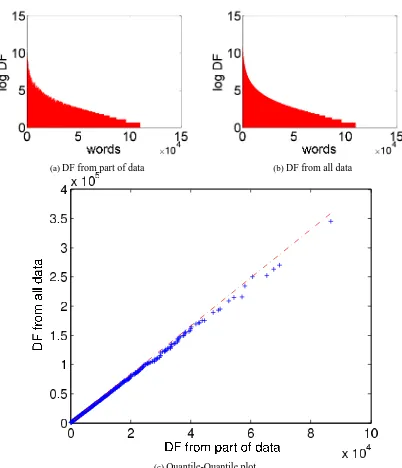
A quantile-quantile plot in Figure 1 shows that this approximation is justified—the dependency between the statistics on the subset (200k articles) and the full training set (800k articles) is perfectly linear.
We compare the hash kernel with Leon Bottou’s Stochastic Gradient Descent SVM2(BSGD), Vowpal Wabbit (Langford et al., 2007) (VW) and Random Projections (RP) (Achlioptas, 2003). Our hash scheme is generating features online. BSGD is generating features offline and learning them online. VW uses BSGD’s preprocessed features and creates further features online. Caching speeds up VW considerably. However, it requires one run of the original VW code for this purpose. RP uses BSGD’s preprocessed features and then creates the new projected lower dimension features. Then it uses BSGD for learning and testing. We compare these algorithms on RCV1 in Table 2.
(a)DF from part of data (b)DF from all data
(c)Quantile-Quantile plot
Figure 1: Quantile-quantile plot of the DF counts computed on a subset (200k documents) and the full data set (800k documents). DF(t)is the number of documents in a collection containing word t.
HLF (228) HLF (224) HF no hash U base P base
error mem error mem error mem mem error error
L2 30.12 2G 30.71 0.125G 31.28 2.25G (219) 7.85G 99.83 85.05 L3 52.10 2G 53.36 0.125G 51.47 1.73G (215) 96.95G 99.99 86.83 Table 5: Misclassification and memory footprint of hashing and baseline methods on DMOZ. HLF: joint hashing of labels and features. HF: hash features only. no hash: direct model (not implemented as too large, hence only memory estimates—we have 1,832,704 unique words). U base: baseline of uniform classifier. P base: baseline of majority vote. mem: memory used for the model. Note: the memory footprint in HLF is essentially independent of the number of classes used.
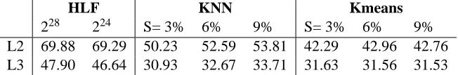
HLF KNN Kmeans
228 224 S= 3% 6% 9% S= 3% 6% 9%
L2 69.88 69.29 50.23 52.59 53.81 42.29 42.96 42.76 L3 47.90 46.64 30.93 32.67 33.71 31.63 31.56 31.53
Table 6: Accuracy comparison of hashing, KNN and Kmeans. HLF: joint hashing of labels and features. KNN: apply K Nearest Neighbor on sampled training set as search set. Kmeans: apply Kmeans on sampled training set to do clustering and then take its majority class as predicted class. S is the sample size which is the percentage of the entire training set.
is considerable compared to disk access. Table 2 shows that the test errors for hash kernel, BSGD and VW are competitive.
In table 3 we compare hash kernel to RP with different feature dimensions. As we can see, the error reduces as the new feature dimension increases. However, the error of hash kernel is always much smaller (by about 10%) than RP given the same new dimension. An interesting thing is that the new feature file created after applying RP is much bigger than the original one. This is because the projection maps the original sparse feature to a dense feature. For example, when the feature dimension is 210, the compressed new feature file size is already 5.8G. Hash kernel is much more efficient than RP in terms of speed, since to compute a hash feature one requires only O(dnz) hashing operations, where dnz is the number of non-zero entries. To compute a RP feature one requires O(dn)operations, where d is the original feature dimension and and n is the new feature dimension. And with RP the new feature is always dense even when n is big, which further increases the learning and testing runtime. When dnz≪d such as in text process, the difference is significant. This is verified in our experiment (see in Table 3). For example, hash kernel (including Pre and TrainTest) with 210feature size is over 100 times faster than RP.
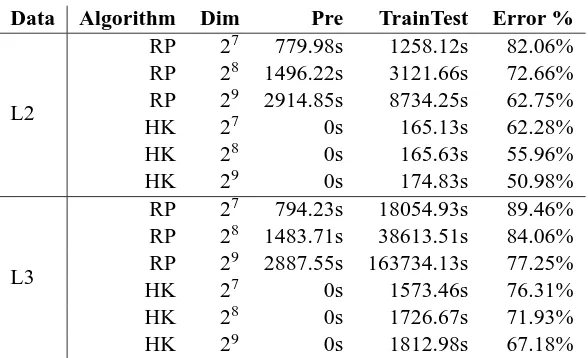
Data Algorithm Dim Pre TrainTest Error %
L2
RP 27 779.98s 1258.12s 82.06%
RP 28 1496.22s 3121.66s 72.66%
RP 29 2914.85s 8734.25s 62.75%
HK 27 0s 165.13s 62.28%
HK 28 0s 165.63s 55.96%
HK 29 0s 174.83s 50.98%
L3
RP 27 794.23s 18054.93s 89.46%
RP 28 1483.71s 38613.51s 84.06% RP 29 2887.55s 163734.13s 77.25%
HK 27 0s 1573.46s 76.31%
HK 28 0s 1726.67s 71.93%
HK 29 0s 1812.98s 67.18%
Table 7: Hash kernel vs. random projections with various feature dimensionalities on Dmoz. RP: random projections in Achlioptas (2003). HK: hash kernel. Dim: dimension of the new features. Pre: preprocessing time—generation of the random projected features. TrainTest: time to load data, train and test the model. Error: misclassification rate. Note that the TrainTest time for random projections increases as the new feature dimension increases, whereas for hash kernel the TrainTest is almost independent of the feature dimensionality. Moving the dimension from 28to 29 the in-creasing in processing time of RP is not linear—we suspect this is because with 28 the RP model has 256×7100×8≈14MB, which is small enough to fit in the CPU cache (we are using a 4-cores cpu with a total cache size of 16MB), while with 29 the model has nearly 28MB, no longer fitting in the cache.
6.2 Dmoz Websites Multiclass Classification
In a second experiment we perform topic categorization using the DMOZ topic ontology. The task is to recognize the topic of websites given the short descriptions provided on the webpages. To simplify things we categorize only the leaf nodes (Top two levels: L2 or Top three levels: L3) as a flat classifier (the hierarchy could be easily taken into account by adding hashed features for each part of the path in the tree). This leaves us with 575 leaf topics on L2 and with 7100 leaf topics on L3.
Conventionally, assuming M classes and l features, training M different parameter vectors w requires O(Ml) storage. This is infeasible for massively multiclass applications. However, by hashing data and labels jointly we are able to obtain an efficient joint representation which makes the implementation computationally possible.
Figure 2: Test accuracy comparison of KNN and Kmeans on Dmoz with various sample sizes. Left: results on L2. Right: results on L3. Hash kernel (228) result is used as an upper bound.
Next we compare hash kernel with K Nearest Neighbor (KNN) and Kmeans. Running the naive KNN on the entire training set is very slow.3 Hence we introduce sampling to KNN. We first sample a subset from the entire training set as search set and then do KNN classification. To match the scheme of KNN, we use sampling in Kmeans too. Again we sample from the entire training set to do clustering. The number of clusters is the minimal number of classes which have at least 90% of the documents. Each test example is assigned to one of the clusters, and we take the majority class of the cluster as the predicted label of the test example. The accuracy plot in Figure 2 shows that in both Dmoz L2 and L3, KNN and Kmeans with various sample sizes get test accuracies of 30% to 20% off than the upper bound accuracy achieved by hash kernel. The trend of the KNN and Kmeans accuracy curve suggests that the bigger the sample size is, the less accuracy increment can be achieved by increasing it. A numerical result with selected sample sizes is reported in Table 6.
We also compare hash kernel with RP with various feature dimensionality on Dmoz. Here RP generates the random projected feature first and then does online learning and testing. It uses the same 4-cores implementation as hash kernel does. The numerical result with selected dimensional-ities is in Table 7. It can be seen that hash kernel is not only much faster but also has much smaller error than RP given the same feature dimension. Note that both hash kernel and RP reduce the error as they increase the feature dimension. However, RP can’t achieve competitive error to what hash kernel has in Table 5, simply because with large feature dimension RP is too slow—the estimated run time for RP with dimension 219on dmoz L3 is 2000 days.
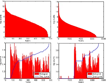
Furthermore we investigate whether such a good misclassification rate is obtained by predicting well only on a few dominant topics. We reorder the topic histogram in accordance to ascending error rate. Figure 3 shows that hash kernel does very well on the first one hundred topics. They correspond to easy categories such as language related sets ”World/Italiano”,”World/Japanese”,”World/Deutsch”.
3. In fact the complexity of KNN is O(N×T), where N,T are the size of the training set and the testing set. We estimate
Figure 3: Left: results on L2. Right: results on L3. Top: frequency counts for topics as reported on the training set (the test set distribution is virtually identical). We see an exponential decay in counts. Bottom: log-counts and error probabilities on the test set. Note that the error is reasonably evenly distributed among the size of the classes (besides a number of near empty classes which are learned perfectly).
6.3 Biochemistry and Bioinformatics Graph Classification
For the final experiment we work with graphs. The benchmark data sets we used here contain three real-world data sets: two molecular compounds data sets, Debnath et al. (1991) and PTC (Toivonen et al., 2003), and a data set for protein function prediction task (DD) from Dobson and Doig (2003). In this work we used the unlabeled version of these graphs, see, for example, Borgwardt et al. (2007).
Data Sets RW SP GKS GK HK HKF MUTAG 0.719 0.813 0.819 0.822 0.855 0.865 PTC 0.554 0.554 0.594 0.597 0.606 0.635 DD >24h >24h 0.745 >24h 0.799 0.841
Table 8: Classification accuracy on graph benchmark data sets. RW: random walk kernel, SP: short-est path kernel, GKS = graphlet kernel sampling 8497 graphlets, GK: graphlet kernel enumerating all graphlets exhaustively, HK: hash kernel, HKF: hash kernel with feature selection. ’>24h’ means computation did not finish within 24 hours.
Feature All Selection
STATS ACC AUC ACC AUC
MUTAG 0.855 0.93 0.865 0.912
PTC 0.606 0.627 0.635 0.670
DD 0.799 0.81 0.841 0.918
Table 9: Non feature selection vs feature selection for hash kernel. All: all features. Selection: feature selection; ACC: accuracy; AUC: Area under ROC.
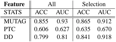
We compare the proposed hash kernel (with/without feature selection) with random walk kernel, shortest path kernel and graphlet kernel on the benchmark data sets. From Table 8 we can see that the hash Kernel even without feature selection still significantly outperforms the other three kernels in terms of classification accuracy over all three benchmark data sets.
The dimensionality of the canonical isomorph representation is quite high and many features are extremely sparse, a feature selection step was taken that removed features suspected as non-informative. To this end, each feature was scored by the absolute vale of its correlation with the target. Only features with scores above median were retained. As can be seen in Table 9 feature selection on hash kernel can furthermore improve the test accuracy and area under ROC.
7. Discussion
In this paper we showed that hashing is a computationally attractive technique which allows one to approximate kernels for very high dimensional settings efficiently by means of a sparse projection into a lower dimensional space. In particular for multiclass categorization this makes all the differ-ence in terms of being able to implement problems with thousands of classes in practice on large amounts of data and features.
References
D. Achlioptas. Database-friendly random projections:johnson-lindenstrauss with binary coins. Journal of Computer and System Sciences, 66:671C687, June 2003.
C. Berg, J. P. R. Christensen, and P. Ressel. Harmonic Analysis on Semigroups. Springer, New York, 1984.
B. H. Bloom. Space/time trade-offs in hash coding with allowable errors. Communications of the ACM, 13:422C426, July 1970.
K. M. Borgwardt, H.-P. Kriegel, S. V. N. Vishwanathan, and N. Schraudolph. Graph kernels for dis-ease outcome prediction from protein-protein interaction networks. In Russ B. Altman, A. Keith Dunker, Lawrence Hunter, Tiffany Murray, and Teri E Klein, editors, Proceedings of the Pacific Symposium of Biocomputing 2007, Maui Hawaii, January 2007. World Scientific.
C. J. C. Burges and B. Sch¨olkopf. Improving the accuracy and speed of support vector learning machines. In M. C. Mozer, M. I. Jordan, and T. Petsche, editors, Advances in Neural Information Processing Systems 9, pages 375–381, Cambridge, MA, 1997. MIT Press.
G. Cormode and M. Muthukrishnan. An improved data stream summary: The count-min sketch and its applications. In LATIN: Latin American Symposium on Theoretical Informatics, 2004.
A. K. Debnath, R. L. Lopez de Compadre, G. Debnath, A. J. Shusterman, and C. Hansch. Structure-activity relationship of mutagenic aromatic and heteroaromatic nitro compounds. correlation with molecular orbital energies and hydrophobicity. J Med Chem, 34:786–797, 1991.
O. Dekel, S. Shalev-Shwartz, and Y. Singer. The Forgetron: A kernel-based perceptron on a fixed budget. In Y. Weiss, B. Sch¨olkopf, and J. Platt, editors, Advances in Neural Information Process-ing Systems 18, Cambridge, MA, 2006. MIT Press.
P. D. Dobson and A. J. Doig. Distinguishing enzyme structures from non-enzymes without align-ments. J Mol Biol, 330(4):771–783, Jul 2003.
S. Fine and K. Scheinberg. Efficient SVM training using low-rank kernel representations. JMLR, 2:243–264, Dec 2001.
K. Ganchev and M. Dredze. Small statistical models by random feature mixing. In workshop on Mobile NLP at ACL, 2008.
P. Indyk and R. Motawani. Approximate nearest neighbors: Towards removing the curse of di-mensionality. In Proceedings of the 30th Symposium on Theory of Computing, pages 604–613, 1998.
L. Kontorovich. A universal kernel for learning regular languages. In Machine Learning in Graphs, 2007.
J. Langford, L. Li, and A. Strehl. Vowpal wabbit online learning project (technical report). Technical report, 2007.
D.D. Lewis, Y. Yang, T.G. Rose, and F. Li. Rcv1: A new benchmark collection for text categoriza-tion research. The Journal of Machine Learning Research, 5:361–397, 2004.
O. L. Mangasarian. Generalized support vector machines. Technical report, University of Wiscon-sin, Computer Sciences Department, Madison, 1998.
B. D. McKay. nauty user’s guide. Technical report, Dept. Computer Science, Austral. Nat. Univ., 1984.
A. Nobel and A. Dembo. A note on uniform laws of averages for dependent processes. Statistics and Probability Letters, 17:169–172, 1993.
N. Przulj. Biological network comparison using graphlet degree distribution. Bioinformatics, 23 (2):e177–e183, Jan 2007.
A. Rahimi and B. Recht. Random features for large-scale kernel machines. In J.C. Platt, D. Koller, Y. Singer, and S. Roweis, editors, Advances in Neural Information Processing Systems 20. MIT Press, Cambridge, MA, 2008.
B. Sch¨olkopf. Support Vector Learning. R. Oldenbourg Verlag, Munich, 1997. Download: http://www.kernel-machines.org.
J. Shawe-Taylor and N. Cristianini. Kernel Methods for Pattern Analysis. Cambridge University Press, Cambridge, UK, 2004.
Q. Shi, J. Petterson, G. Dror, J. Langford, A. Smola, A. Strehl, and S. V. N. Vishwanathan. Hash ker-nels. In Max Welling and David van Dyk, editors, Proc. Intl. Workshop on Artificial Intelligence and Statistics. Society for Artificial Intelligence and Statistics, 2009.
C. H. Teo and S. V. N. Vishwanathan. Fast and space efficient string kernels using suffix arrays. In ICML ’06: Proceedings of the 23rd international conference on Machine learning, pages 929– 936, New York, NY, USA, 2006. ACM Press. ISBN 1-59593-383-2. doi: http://doi.acm.org/10. 1145/1143844.1143961.
H. Toivonen, A. Srinivasan, R. D. King, S. Kramer, and C. Helma. Statistical evaluation of the predictive toxicology challenge 2000-2001. Bioinformatics, 19(10):1183–1193, July 2003.
K. Tsuda, T. Kin, and K. Asai. Marginalized kernels for biological sequences. Bioinformatics, 18 (Suppl. 2):S268–S275, 2002.
S. V. N. Vishwanathan, Karsten Borgwardt, and Nicol N. Schraudolph. Fast computation of graph kernels. In B. Sch¨olkopf, J. Platt, and T. Hofmann, editors, Advances in Neural Information Processing Systems 19, Cambridge MA, 2007a. MIT Press.
S. V. N. Vishwanathan, A. J. Smola, and R. Vidal. Binet-Cauchy kernels on dynamical systems and its application to the analysis of dynamic scenes. International Journal of Computer Vision, 73 (1):95–119, 2007b.