Magic Moments for Structured Output Prediction
Elisa Ricci [email protected]
Dept. of Electronic and Information Engineering University of Perugia
06125 Perugia, Italy
Tijl De Bie [email protected]
Dept. of Engineering Mathematics University of Bristol
Bristol, BS8 1TR, UK
Nello Cristianini [email protected]
Dept. of Engineering Mathematics and Dept. of Computer Science University of Bristol
Bristol, BS8 1TR, UK
Editor: Michael Collins
Abstract
Most approaches to structured output prediction rely on a hypothesis space of prediction functions that compute their output by maximizing a linear scoring function. In this paper we present two novel learning algorithms for this hypothesis class, and a statistical analysis of their performance. The methods rely on efficiently computing the first two moments of the scoring function over the output space, and using them to create convex objective functions for training. We report exten-sive experimental results for sequence alignment, named entity recognition, and RNA secondary structure prediction.
Keywords: structured output prediction, discriminative learning, Z-score, discriminant analysis,
PAC bound
1. Introduction
The last few years have seen a growing interest in learning algorithms that operate over structured data: given a set of training input-output pairs, they learn to predict the output corresponding to a previously unseen input, where either the input or the output (or both) are more complex than traditional data types such as vectors.
Examples of such problems abound: learning to align biological sequences, learning to parse strings, learning to translate natural language, learning to find the optimal route in a graph, learning to understand speech, and much more. This problem setting subsumes as a special case the standard regression, binary classification, and multiclass classification problems. In fact in many cases the structured output prediction approach matches practice more closely. However, this broad generality and applicability comes with a number of significant theoretical and practical challenges.
with each other. Because of this, even the prediction task itself requires a search (or optimization) over the complete output space, which in itself is often nontrivial. A fortiori, the task of learning to predict poses important new challenges in comparison with standard machine learning approaches such as regression and classification.
1.1 Graphical and Grammatical Models for Structured Data
An immediate approach for structured output prediction would be to use a probabilistic model jointly over the input and the output variables. Probabilistic graphical models (PGMs) or stochastic context free grammars (SCFGs) are two examples of techniques that allow one to specify proba-bilistic models for a variety of inputs and outputs, explicitly encoding the structure that is present. For a given input, the predicted output can then be found as the one that maximizes the a posteriori probability. This way of predicting structured outputs is referred to as maximum a posteriori (MAP) estimation. The learning phase then boils down to modeling the distribution of the joint of input and output data.
However, it is well known that this indirect approach of first modeling the distribution (dis-regarding the prediction task of interest) and subsequently using MAP estimation for prediction, risks to be suboptimal. Instead a direct discriminative approach is more appropriate, which directly focuses on the prediction task of interest. Such methods, known as discriminative learning algo-rithms (DLAs), make predictions by optimizing a scoring function over the output space, where this scoring function has not necessarily a probabilistic interpretation.
Recently studied DLAs include maximum entropy Markov models (McCallum et al., 2000), conditional random fields (CRFs) (Lafferty et al., 2001), re-ranking with perceptron (Collins, 2002b), hidden Markov perceptron (HMP) (Collins, 2002a), sequence labeling with boosting (Altun et al., 2003a), maximal margin (MM) algorithms (Altun et al., 2003b; Taskar et al., 2003; Tsochantaridis et al., 2005), Gaussian process models (Altun et al., 2004), and kernel conditional random fields (Lafferty et al., 2004).
Interestingly, both the generative modeling approach and the DLAs mentioned above make use of formally the same hypothesis class of prediction functions. In particular, they all make use of a scoring function that is linear in a set of parameters to score each element of the output space. In the generative approach, this linear function is the log-probability of the joint of the input and output data; in the discriminative approach this can be any linear function. The actual prediction function then selects the output that achieves the highest value of the scoring function (i.e., the highest score). In the generative approach this means that the a posteriori (log)-probability of the output is maximized, such that the MAP estimate is obtained as pointed out above.
1.2 The Contributions of this Paper
In this paper we will adopt the hypothesis space of prediction functions defined as above. The distribution of scores induced by any hypothesis over all possible outputs is a central concept in various approaches, and can be used to compare hypotheses, and hence to train. For example MM approaches (Altun et al., 2003b; Taskar et al., 2003; Tsochantaridis et al., 2005) prescribe to seek hypotheses that make the score of the correct outputs in the training set larger than all incorrect ones (by a certain margin).
choices of parameters can be assessed by comparing (a function of) those moments. Such an ap-proach would account for all possible output values at once, rather than just the ones with a high score as in the maximum margin approaches. However these moments cannot be computed by brute force enumeration: in all practical cases the output space is far too large to exhaustively tra-verse it. Nevertheless in this paper we show how the first and second order moments can often be computed efficiently by means of dynamic programming (DP), without explicitly enumerating the output space. We provide specific examples of how these moments can be computed for three types of structured output prediction problems: the sequence alignment problem, sequence labeling, and learning to parse with a context free grammar for RNA secondary structure prediction.
We then present two ways in which these moments can be used to design a convex objective function for a learning algorithm. The first approach is the maximization of the Z-score, a common statistical measure of surprise, which is large if the scores of the correct outputs in the training set are significantly different from the scores of all incorrect outputs in the output space. We show that the Z-score is a convex cost function, such that it can be optimized efficiently. A second approach— also convex—is reminiscent of Fisher’s discriminant analysis (FDA). We call this new algorithm SODA (structured output discriminant analysis) since the optimization criterion is a similar function of the first and second order statistics as in FDA.
We report extensive experimental results for the proposed algorithms applied to three different problem settings: learning to align, sequence labeling, and RNA folding.
Finally we derive learning-theoretic bounds on the performance of these algorithms, showing that the SODA cost function is related to the rank of the correct output among the other outputs and analyzing its statistical stability within the Rademacher framework; additionally, we present a general PAC bound that applies to any algorithm using this hypothesis class.
1.3 Outline of this Paper
The rest of the paper is structured as follows: Section 2 formally introduces the problem of struc-tured output learning and the hypothesis space considered. Section 3 deals with the computation of the first and second order moments of the score distribution through DP. In Section 4 we introduce the two algorithms. In Section 5 we present our experimental results, and in Section 6 we outline learning-theoretical bounds, whose proof is however left for the appendix.
2. Learning to Predict Structured Outputs
We address the general problem of learning a prediction function h :
X
→Y
, withY
a potentially highly structured space containing a potentially large number N of elements. The learning is based on a training set of input-output pairsT
={(x1,¯y1),(x2,¯y2), . . . ,(x`,¯y`)}drawn i.i.d. from some2.1 Scoring Functions, Prediction Functions, and the Hypothesis Space
As in standard machine learning approaches, we consider learning methods that choose the pre-diction function from a hypothesis space by minimizing a cost function evaluated on the training data. To establish the type of hypothesis space we will consider, we will rely on the notion scoring function, which is a function s :
X
×Y
→Rthat assigns a numerical score s(x,y)to a pair(x,y)of input-output variables. Furthermore, we will assume that s is linear in a parameter vectorθ∈Rd:Definition 1 (Linear scoring function) A linear scoring function is a function sθ :
X
×Y
→Rdefined as:
sθ(x,y) =θTφ(x,y), (1)
where the vectorφ(x,y) = (φ1(x,y),φ2(x,y), . . . , φd(x,y))T is defined by a specified set of integer-valued feature functionsφi:
X
×Y
→[0,C]for a fixed upper bound C.Based on this, we can define prediction functions as considered in this paper as follows:
Definition 2 (Prediction function) Given a linear scoring function sθ, we can define a prediction function hθ:
X
→Y
as:hθ(x) =arg max
y∈Y sθ(x,y). (2)
This type of prediction function has been used in previous approaches for structured output predic-tion. For example, when using a discrete-valued PGM to model the joint distribution of the input and output data, the logarithm of the probability distribution is a linear scoring function as defined above. The vectorφ(x,y)is then the vector of sufficient statistics, and the parameter vectorθ corre-sponds to the logarithms of the clique potentials or conditional probabilities. Then, a MAP estimator corresponds to a prediction function as defined above. Furthermore, note that each feature function φithat counts a sufficient statistic is either an indicator function, or the sum of an indicator function evaluated on a set of cliques over which the parameterθiis reused. Therefore, each of the features must be an integer between 0 and the number of cliques C, as required for linear scoring functions in Definition 1.
Typically, in PGMs the parametersθwould be inferred by Maximum Likelihood. On the con-trary in DLAsθis computed by minimizing criteria that are more directly linked to the prediction performance. Moreover with DLAs richer feature vectors (with features not necessarily associated to clique potentials or conditional probabilities) are allowed to describe more effectively the relation between input and output variables. This means that the score sθ(x,y)looses its interpretation as a log-likelihood function.
In summary, the hypothesis space we consider in this paper is defined as:
H
={hθ:θ∈Rd}. (3)This is a slightly larger hypothesis space as compared to the one considered in PGMs, since the parametersθare not restricted to represent log probabilities.
output space
Y
. In fact, it is often convenient to define or derive the scoring function starting from a PGM, to ensure that it is easily maximized by a dynamic programming procedure such as the Viterbi algorithm. Subsequently the constraints on the parameters that are meant to guarantee that the scoring function is a log-probability function can be removed, in order to arrive at a hypothesis space of the form (3).2.2 Ideal Loss Functions
In order to select an appropriate prediction function from the hypothesis space, a cost function needs to be defined. Here we will provide an overview of a few conceptually interesting cost functions, but which are unfortunately hard to optimize. Nevertheless, they can often be approximated as seen from literature, and as we will demonstrate further on.
Consider a loss function
L
θ that maps the input x and the true training output ¯y to a positive real numberLθ
(x,¯y), in some way measuring the discrepancy between the prediction hθ(x)and ¯y. Empirical risk minimization strategies attempt to find the vectorθ∈Rdsuch that the empirical risk, defined as:Rθ
(T
) =1`
`
∑
i=1
Lθ
(xi,¯yi)is minimized, in hopes that this will guarantee that the expected loss E{
Lθ
(x,¯y)}is small as well. Often it is beneficial to introduce regularization in order to prevent overfitting to occur, but let us first consider on the empirical risk itself.Clearly the choice of the loss function is critical, and different choices may be appropriate in dif-ferent situations. The simplest one is a natural extension of the zero-one loss in binary classification task, defined as:
L
ZOθ (x,¯y) = I(hθ(x)6=¯y)
where I(·)is an indicator function. Unfortunately the zero-one loss function is discontinuous and NP-hard to optimize. Therefore algorithms such as CRFs (Lafferty et al., 2001) and MM methods (Altun et al., 2003b) minimize an upper bound on this loss rather than the loss itself, combined with an appropriate regularization term.
However, in structured output prediction, the zero-one loss is quite crude, in the sense that it makes no distinction in the type of mistake that has been made. For example, assume that the outputs y are sequences of length m, or vectors: y= (y1,y2, . . . ,ym). In that case, a wrong prediction is likely to be less damaging if it is due to only one or a few incorrectly predicted symbols in the sequence. A better loss function that distinguishes incorrect predictions in this way is the Hamming loss, originally proposed in Taskar et al. (2003) for MM algorithms:
L
Hθ (x,¯y) =
∑
jI(hθ,j(x)6=y¯j),
counting the number of elements (i.e., the symbols in a sequence, or coordinates in a vector) of the output where a mistake has been made.
totally different stable fold states, both with functional relevance. Therefore, where perfect predic-tion of the data cannot be achieved using the hypothesis space considered, it could be more useful to measure the fraction of outputs for which the score is ranked higher than for the correct output. This is the main motivation to use what we call the relative ranking (RR) loss:
L
RRθ (x,¯y) =N1 N
∑
j=1
I(s(x,¯y)≤s(x,yj)),
We refer to this loss as the relative ranking loss, since the rank divided by the total size of the output space N is computed. This loss and related loss functions have been proposed in Freund et al. (1998), Schapire and Singer (1999) and Altun et al. (2003a).
2.3 Playing with Sequences: Labeling, Aligning and Parsing
In order to further clarify the framework of structured output learning we present three typical problems which we will use in the rest of the paper as illustrative examples: sequence labeling learning, sequence alignment learning and parse learning.
2.3.1 SEQUENCELABELINGLEARNING
In sequence labeling tasks a sequence is taken as an input, and the output to be predicted is a se-quence that annotates the input sese-quence, that is, with a symbol corresponding to each symbol in the input sequence. This problem arises in several application such as gene finding or protein struc-ture prediction in computational biology or named entity recognition and part of speech tagging in the natural language processing field. Traditionally a special type of PGM, namely hidden Markov models (HMMs) (Rabiner, 1989), is used in sequence labeling, where the parameters can be learned by maximum likelihood, and subsequently predictions can be made by MAP estimation. In order to derive a DLA for this setting, we will first derive the prediction function corresponding to MAP estimation based on HMMs, and subsequently remove the constraints on the parameters that allow for the probabilistic interpretation of HMMs. Then an appropriate cost function for discrimination can be optimized to select a good parameter setting.
In an HMM (Fig. 1) there is a sequence of observed variables x= (x1,x2, ...,xm) ∈
X
which will be the input in the terminology of the paper, along with a sequence of corresponding hidden variables y= (y1,y2, ...,ym) ∈Y
, in the present terminology corresponding to the output sequence to be predicted. Each observed symbol xi is an element of the observed symbol alphabet Σx, and the hidden symbols yiare elements ofΣy, with no=|Σx|and nh=|Σy|the respective alphabet sizes. Therefore the output space isY
=Σym, whileX
=Σxm. The number of cliques C=2m−1 of the HMM graphical model is equal to the number of edges.Figure 1: The graph of an HMM with m=4.
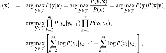
likely given the observation sequence x. In formulas:
h(x) = arg max
y∈YP(y|x) =arg maxy∈Y P(y,x)
P(x) =arg maxy∈YP(y)P(x|y),
= arg max
y∈Y m
∏
k=2
P(yk|yk−1) m
∏
k=1
P(xk|yk),
= arg max
y∈Y
" m
∑
k=2
log P(yk|yk−1) + m
∑
k=1
log P(xk|yk) #
,
where we made use of the fact that the argmax of a function is equal to the argmax of its logarithm. Thus, to fully specify the HMM, one needs to consider all the transition probabilities (denoted ti j for i,j∈Σyfor the transition from symbol i to j), and the emission probabilities (denoted eiofor the emission of symbol o∈Σxby symbol i∈Σy). Using this notation, we can rewrite the prediction function as follows (with I(·)equal to one if the equalities between brackets hold):
h(x) = arg maxy∈Y
∑
i,j∈Σy log(ti j)
m
∑
k=2
I(yk−1=i,yk=j)
+
∑
i∈Σy,o∈Σx
log(eio) m
∑
k=1
I(yk=i,xk=o).
For simplicity of notation let us replace all logarithms of parameters ti j and eio by parameters θi summarized in a d =nhno+n2h dimensional parameter vector θ. Additionally, let us summa-rize the corresponding sufficient statistics ∑mk=2I(yk−1=i,yk = j) and∑mk=1I(yk =i,xk =o) in a corresponding feature vectorφ(x,y) = [φ1(x,y)φ2(x,y) . . . φd(x,y)]T. (Note that these sufficient statistics count the number of occurrences of each specific transition and emission.) Then we can rewrite the prediction function in a linear form as required:
hθ(x) = arg max y∈Y θ
Tφ(x,y).
vectorφ(x,y)contains not only statistics associated to transition and emission probabilities but also any feature that reflects the properties of the objects represented by the nodes of the HMM. For example in most of the natural language processing tasks, feature vectors also contain information about spelling properties of words. Sometimes also the so-called ‘overlapping features’ (Lafferty et al., 2001) are employed, which indicate relations between observations and some previous and future labels. Most of DLAs dealing with this task have proceeded in this way (McCallum et al., 2000; Lafferty et al., 2001; Collins, 2002a; Altun et al., 2003a,b; Taskar et al., 2003).
2.3.2 SEQUENCEALIGNMENTLEARNING
As second case studied, we consider the problem of learning how to align sequences: given as training examples a set of correct pairwise global alignments, find the parameter values that ensure sequences are optimally aligned. This task is also known as inverse parametric sequence alignment problem (IPSAP) and since its introduction in Gusfield et al. (1994), it has been widely studied (Gusfield and Stelling, 1996; Kececioglu and Kim, 2006; Joachims et al., 2005; Pachter and Sturm-fels, 2004; Sun et al., 2004).
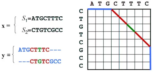
Consider two strings S1 and S2 of lengths n1 and n2 respectively. The strings are ordered se-quences of symbols si ∈
S
, withS
a finite alphabet of size nS. In case of biological applications, for DNA sequences the alphabet contains the symbols associated with nucleotides (S
={A,C,G,T}), while for amino acids sequences the alphabet isS
={A,R,N,D,C,Q,E,G,H,I,L,K,M,F,P,S,T,W,Y,V}. An alignment of two strings S1and S2of lengths n1and n2is defined as a pair of sequences T1 and T2 of equal length n≥n1,n2 that are obtained by taking S1 and S2 respectively and inserting symbols−at various locations in order to arrive at strings of length n. Two symbols in T1 and T2 are said to correspond if they occur at the same location in the respective string. If corresponding symbols are equal, this is called a match. If they are not equal, this is a mismatch. If one of the symbols is a−, this is called a gap.With each possible match, mismatch or gap a score is attached. To quantify these scores, three score parameters can be used: one for matches (θm), one for mismatches (θs), and one for gaps (θg). In analogy with the notation in this paper, the pair of given sequences S1and S2represent the input variable x while their alignment is the output y. The score of the global alignment is defined as the sum of this score over the length of T1 and T2, that is, as a linear function of the alignment parameters:
sθ(x,y) =θTφ(x,y) =θmm+θss+θgg
whereφ(x,y) = [m s g]Tand m, s and g represent the number of matches, mismatches and gaps in the alignment. Fig. 2 depicts a pairwise alignment between two sequences and the associated path in the alignment graph. The number N of all possible alignments between S1and S2is clearly exponential in the size of the two strings. However, an efficient DP algorithm for computing the alignment with maximal score ¯y is known in literature: the Needleman-Wunsch algorithm (Needleman, 1970).
The scoring models presented above consider a local form of gap penalty: the gap penalty is fixed independently of the other gaps in the alignment. However for biological reasons it is often preferable to consider an affine function for gap penalties, that is to assign different costs if the gap starts (gap opening penaltyθo) in a given position or if it continues (gap extension penaltyθe). Then the score of an alignment is:
Figure 2: An alignment y between two sequences S1 and S2 can be represented by a path in the alignment graph.
where m, s, o and e represent the number of match, mismatch, gap openings and gap extensions respectively andθm, θs, θo, θe are the associated costs. As before we can define the vectors θ= [θmθsθoθe]Tandφ(x,y) = [m s o e]T. Therefore the score is still a linear function of the parameters and the prediction can be computed by a DP algorithm.
More often a different model is considered where a (symmetric) scoring matrix specifies dif-ferent score values for each possible pair of symbols. In general there are d= nS(n2S+1) different parameters inθassociated with the symbols of the alphabet plus two additional ones corresponding to the gap penalties. This means that to align sequences of amino acids we have 210 parameters to determine plus other 2 parameters for gap opening and gap extension. We denote with zjk the number of pairs where a symbol of T1is j and it corresponds to a symbol k in T2. Again the score is a linear function of the parameters:
sθ(x,y) =
∑
j≥kθjkzjk+θoo+θee
and the optimal alignment is computed by the Needleman-Wunsch algorithm.
2.3.3 LEARNING TOPARSE
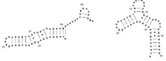
In learning to parse the input x is given by a sequence, and the output is given by its associated parse tree according to a context free grammar. Usually weighted context-free grammars (WCFGs) (Manning and Schetze, 1999) are used to approach this problem. Learning to parse has been already studied as a particular instantiation of structured output learning, both in natural language processing applications (Tsochantaridis et al., 2005; Taskar et al., 2004) and in computational biology for RNA secondary structure alignment (Sato and Sakakibara, 2005) and prediction (Do et al., 2006). In this paper we consider the latter and we use WCFGs to model the structure of RNA sequences. Two examples of RNA secondary structure for two sequences are shown in Fig. 3.
Figure 3: Two examples of RNA secondary structures for two sequences of the Rfam database (Griffiths-Jones et al., 2003).
S∈ϒis the starting symbol, andθis a set of weights. We use rules of the formsϒi→X ,ϒi→ϒjϒk, ϒi→XϒjX0, andϒi→ϒj0 ( j0>i). R is also indexed by an ordering{r1, . . . ,r|R|}and d=|R|. Each
node in the parse tree y corresponds to a grammar rule and each weightθi∈θis associated with a rule ri∈R. Given a sequence x and an associated parse tree y we can define a feature vectorφ(x,y) which contains a count of the number of occurrences of each of the rules in the parse tree y. Given a parameter vectorθ, the prediction function hθ(x)is computed by finding the best parse tree. For SCFGs, this can be done efficiently with the Cocke-Younger-Kasami (CYK) algorithm (Younger, 1967).
3. Computing the Moments of the Scoring Function
An interesting corollary of the proposed structured output approach based on linear scoring func-tions is that certain statistics of the score s(x,y)can be expressed as function of the parameter vector θ. More specifically given an observed vector x, we can consider the first order moment or mean M1,θ(x)and the centered second order moment or covariance M2,θ(x)of the scores along all
pos-sible N output variables yj. It is straightforward to see that M1,θ(x)is a linear function ofθ, that
is,
M1,θ(x) ,
1 N
N
∑
j=1
sθ(x,yj)
= θT 1 N
N
∑
j=1
φ(x,yj)
= θTµ
with µ= [µ1. . .µd]T= 1 N∑
N
j=1φ(x,yj). Similarly, for the covariance: M2,θ(x) ,
1 N
N
∑
j=1
(sθ(x,yj)−M1,θ(x))2
= θT 1 N
N
∑
j=1
(φ(x,yj)−µ)(φ(x,yj)−µ)T !
= θTCθ.
The matrix C is a matrix with elements:
cpq = 1 N
N
∑
j=1
(φp(x,yj)−µp)(φq(x,yj)−µq) (4)
= 1 N
N
∑
j=1
φp(x,yj)φq(x,yj)
−µpµq=vpq−µpµq
where 1≤p,q≤d.
3.1 Magic Moments
It should be clear that in practical structured output learning problems the number N of possible output vectors associated to a given input x can be massive. At first sight, this leaves little hope that the above sums can ever be computed for realistic problems. However, it turns out that the same ideas that allow one to perform inference in PGMs allow one to compute these sums efficiently using DP, be it with somewhat more complicated recursions.
The underlying ideas to derive the recursions for µ are based on the commutativity of the semi-ring that is used in the Viterbi (or more generally the max-product and related algorithms) in PGMs. In particular, this recursion is used in various forms:
E (
k
∑
i=1 ai
)
= E (
k−1
∑
i=1 ai
)
+E{ak},
where the expectations are jointly over independent random variables ai. For the recursions for the second order moment (which can be used to compute the centered second order moment as shown in (4)), the following recursive expression is applied in different variations:
E
k
∑
i=1 ai
!2
= E
k−1
∑
i=1 ai
!2 +2E
( ak
k−1
∑
i=1 ai
)
+Ea2k ,
where again the expectations are jointly over independent random variables ai. Note that the middle term on the right hand side is computed by previous iterations for the first order moment. For concreteness, we will now consider separately the three illustrative scenarios introduced above.
3.2 Sequence Labeling Learning
Given a fixed input sequence x, we show here for the sequence labeling example that the elements of µ and C can be computed exactly and efficiently by dynamic programming routines.
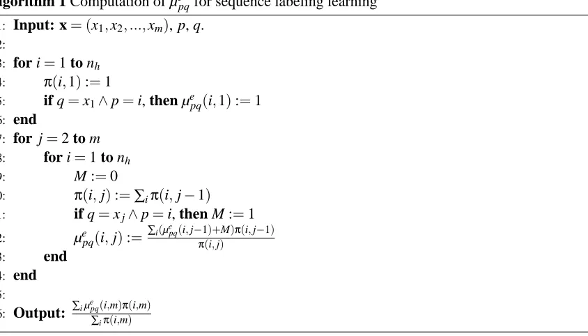
We first consider the vector µ and construct it in a way that the first nhnoelements contain the mean values associated with the emission probabilities and the remaining n2helements correspond to transition probabilities. Each value of µ can be determined by Algorithm 1.
table correspond to a node of the HMM trellis. At the same time another nh×m DP table, denoted byπ, is considered and filled in a way that each elementπ(i,j)contains the number of all possible paths in the HMM trellis terminating at position(i,j). Then a recursive relation is considered to compute each element µepq(i,j),∀1≤ j≤m,∀1≤i≤nh. Basically at step(i,j) the mean value µepq(i,j)is given summing the occurrences of emission probabilities epqat the previous steps (e.g., ∑iµepq(i,j−1)π(i,j−1)) with the number of paths in the previous steps (if the current observation xj is q and the current state yj is p) and dividing this quantity byπ(i,j).
In a similar way the mean values associated to the transition probabilities are computed. Dy-namic programming tables µtpz, 1≤p,z≤nh are filled with recursive formulas in Algorithm 4 in appendix E.
Analogously the elements of the covariance matrix C can be obtained. We have five sets of values: variances of emission probabilities (cepq, 1≤ p≤nh,1≤q≤no), variances of transition probabilities (ctpz, 1≤p,z≤nh), covariances of emission probabilities (cepqp0q0, 1≤p,p0≤nh,1≤
q,q0≤no), covariances of transition probabilities (ctpzp0z0, 1≤p,p0,z,z0≤nh) and mixed covariances
(cetpqp0z, 1≤p,p0,z≤nh,1≤q≤no). To determine each of them we consider (4) and we compute the values ve
pq, vtpz, vepqp0q0, vtpzp0z0 and vetpqp0zsince the mean values are already known. This computation
is again performed following Algorithm 1 but with recursive relations given in Algorithm 4, in appendix E (the number 5, 11, 12 in Algorithm 4 are meant to indicate the lines of Algorithm 1 where the formulas must be inserted).
Algorithm 1 Computation of µepqfor sequence labeling learning
1: Input: x= (x1,x2, ...,xm), p, q.
2:
3: for i=1 to nh
4: π(i,1):=1
5: if q=x1∧p=i, then µpqe (i,1):=1
6: end
7: for j=2 to m
8: for i=1 to nh
9: M :=0
10: π(i,j):=∑iπ(i,j−1)
11: if q=xj∧p=i, then M :=1
12: µepq(i,j):=∑i(µpqe (i,j−1)+M)π(i,j−1) π(i,j)
13: end
14: end
15:
16: Output: ∑iµ e
pq(i,m)π(i,m) ∑iπ(i,m)
3.2.1 COMPUTATIONALCOST ANALYSIS
Proposition 3 The number of dynamic programming routines required to calculate µ and C in-creases linearly with the size of the observation alphabet.
An outline of proof can be found in appendix A.
Algorithms 1 and 4 assume that the HMM is ‘fully connected’, that is, transitions are allowed from and to any possible hidden states and every symbol can be emitted in every state. However, this condition is often not satisfied in practical applications. We should point out that their adap-tation for such situations is straightforward and involves computing only sums that correspond to allowed paths in the DP table. In this case the number of distinct parameters as well as the compu-tational cost increases with respect to complete models. However this effect may be offset by the fact that each DP becomes less time consuming. Furthermore the mean and the covariance values associated to transition probabilities are independent from observations. To calculate them a closed form expression can be used without the need of running any DP routine.
Moreover usually in most applications the size of the observation alphabet (for example the size of the dictionary in a natural language processing system) is very large while the sequences to be labeled are short. This means that the number of distinct observations in each sequence x is much lower than no. In such cases the number of different values in µ and C scales linearly with it.
We point out that the proposed algorithm can be easily extended to the case of arbitrary features in the vectorφ(x,y)(not only those associated with transition and emission probabilities). To com-pute µ and C in these situations the derivation of appropriate formulas similar to those of µepq, cepq and cetpqp0zis straightforward.
3.2.2 ESTIMATINGµANDCBYRANDOMSAMPLING
Still, the computational cost increases with the number of features since for HMMs that are not ‘fully connected’, it may occur that the number of different values in the matrix C scales quadrat-ically with the observations alphabet size no. However we show that in this case accurate and efficient approximation algorithms can be used to obtain close estimates of the mean and the vari-ance values with a significantly reduced computational cost. This can be achieved by considering a finite subsample of all possible values for the output y, rather than using the DP approaches. This comment holds generally for all learning problems considered in this paper, and we come back to this in the theoretical discussion in 6.1 as well as in the experimental results in 5 to support this claim empirically.
3.3 Sequence Alignment Learning
For the sequence alignment learning task we consider separately the three parameter model, the model with affine gap penalties and the model with substitution matrices.
3.3.1 THESIMPLESTSCORINGSCHEME: MATCH, MISMATCH, GAP
For example each element µm(i,j)is computed dividing the total number of matches by the number of alignments π(i,j). If a match occur in position(i,j) (M=1) the total number of matches at step(i,j)is obtained adding to the number of matches in the previous steps (µm(i,j−1)π(i,j−1), µm(i−1,j−1)π(i−1,j−1) and µm(i−1,j)π(i−1,j)) π(i−1,j−1) times a match. Once the algorithm is terminated, the mean values can be read in the cells µm(n1,n2), µs(n1,n2)and µg(n1,n2). The covariance matrix C is the 3×3 matrix with elements cpq, p,q∈ {m,s,g}and it is symmetric (csg=cgs, cmg=cgm, csm=cms). Each value cpqcan be obtained considering (4) and computing the associated values vpqwith appropriate recursive relations (see Algorithm 2).
3.3.2 AFFINEGAPPENALTIES
As before we can define the vector µ= [µm µs µo µe]T and the covariance matrix C as the 4×4 symmetric matrix with elements cpq with p,q∈ {m,s,o,e}. The values of µ and C are computed with DP. In particular µm, µs, vmm, vms and vss are calculated as above, while the other values are obtained with the formulas in Algorithm 5 in appendix E. The terms vse and vsoare missing since they can be calculated with the same formulas of vme and vmosimply changing M with 1−M and µm with µs. Note that in some situations for low values of(i,j) some terms are not defined (i.e., π(i,j−3) when j=2). In such situations they must be ignored in the computation.
3.3.3 EXTENSION TO AGENERALSCORINGMATRIX
The formulas illustrated in the previous paragraphs can be extended to the case of a general substi-tution matrix with minor modifications. Concerning the mean values, µo and µe are calculated as before. For the others it is:
µzpq(i,j):=
µzpq(i−1,j)π(i−1,j) +µzpq(i,j−1)π(i,j−1) + (µzpq(i−1,j−1) +M)π(i−1,j−1)
π(i,j)
where M=1 when two corresponding symbols in the alignment are equal to p and q or vice versa with p,q∈
S
. The matrix C is a symmetric matrix 212×212. The values veo, vee and voo are calculated as above. The derivation of formulas for vzpqzp0q0 is straightforward from vms considering the appropriate values for M and the mean values. The formulas for vzoand vzefollow with minor modification from vmoand vme.3.4 Learning to Parse
For a given input string x, let µp and cpqbe the mean of occurrences of rule p and the covariance between the numbers of occurrences of rules p and q, respectively, that is, the elements of µ and C. The following relations hold:
µp = 1 N
N
∑
j=1
φp(x,yj) = 1 Nψp,
ncpq = 1 N
N
∑
j=1
φp(x,yj)φq(x,yj)
−µpµq= 1
Nγpq−µpµq,
where N is the number of all possible parse trees associated to x,ψpis the number of occurrences of the rule p in all the parse tree yj given x, andγpqdenotes the cooccurrences of p and q.
Algorithm 2 Computation of µ and C with matches, mismatches and gaps.
1: Input: a pair of sequences S1and S2.
2:
3: π(0,0):=1
4: µm(0,0) =µs(0,0) =µg(0,0):=0
5: vmm(0,0) =vms(0,0) =vss(0,0) =vsg(0,0) =vmg(0,0) =vgg(0,0):=0
6: for i=1 : n1
7: π(i,0):=1
8: µg(i,0):=µg(i−1,0) +1
9: vgg(i,0):=vgg(i−1,0) +2µg(i−1,0) +1
10: end
11: for j=1 : n2
12: π(0,j):=1
13: µg(0,j):=µg(0,j−1) +1
14: vgg(0,j):=vgg(0,j−1) +2µg(0,j−1) +1
15: end
16: for i=1 : n1
17: for j=1 : n2
18: π(i,j):=π(i−1,j−1) +π(i,j−1) +π(i−1,j)
19: if s1(i) =s2(j)then M :=1 else M :=0
20: µm(i,j):=µm(i−1,j)π(i−1,j)+µm(i,j−1)π(iπ,(j−i,j1))+(µm(i−1,j−1)+M)π(i−1,j−1)
21: µs(i,j):=µs(i−1,j)π(i−1,j)+µs(i,j−1)π(i,j−π1(i)+(,j)µs(i−1,j−1)+(1−M))π(i−1,j−1)
22: µg(i,j):=µg(i−1,j)+1)π(i−1,j)+(µg(i,j−1)+π(i1,)j)π(i,j−1)+µg(i−1,j−1)π(i−1,j−1)
23: vmm(i,j):=π(i1,j)(vmm(i−1,j)π(i−1,j) +vmm(i,j−1)π(i,j−1)
24: +(vmm(i−1,j−1) +2Mµm(i−1,j−1) +M)π(i−1,j−1))
25: vss(i,j):=π(i1,j)(vss(i−1,j)π(i−1,j) +vss(i,j−1)π(i,j−1)
26: +(vss(i−1,j−1) +2(1−M)µs(i−1,j−1) + (1−M))π(i−1,j−1))
27: vgg(i,j):=π(1i,j)(vgg(i−1,j) +2µg(i−1,j) +1)π(i−1,j)
28: +(vgg(i,j−1) +2µg(i,j−1) +1)π(i,j−1) +vgg(i−1,j−1)π(i−1,j−1))
29: vmg(i,j):=π(i1,j)(vmg(i−1,j) +µm(i−1,j))π(i−1,j) + (vmg(i,j−1)
30: +µm(i,j−1))π(i,j−1) + (vmg(i−1,j−1) +Mµg(i−1,j−1))π(i−1,j−1))
31: vsg(i,j):=π(i1,j)(vsg(i−1,j) +µs(i−1,j))π(i−1,j) + (vsg(i−1,j−1)
32: +(1−M)µg(i−1,j−1) + (vsg(i,j−1) +µs(i,j−1))π(i,j−1))π(i−1,j−1))
33: vms(i,j):=π(i1,j)(vms(i−1,j)π(i−1,j) +vms(i,j−1)π(i,j−1)
34: +(vms(i−1,j−1) +Mµs(i−1,j−1) + (1−M)µm(i−1,j−1))π(i−1,j−1))
35: end
36: end
37:
38: Output: µm(n1,n2), µs(n1,n2), µg(n1,n2),
39: cmm(n1,n2):=vmm(n1,n2)−µm(n1,n2)2,
40: css(n1,n2):=vss(n1,n2)−µm(n1,n2)2,
41: cgg(n1,n2):=vgg(n1,n2)−µm(n1,n2)2,
42: cms(n1,n2):=vms(n1,n2)−µm(n1,n2)µs(n1,n2),
43: cmg(n1,n2):=vmg(n1,n2)−µm(n1,n2)µg(n1,n2),
44: csg(n1,n2):=vsg(n1,n2)−µs(n1,n2)µg(n1,n2)
compute the number of parse trees N, another the number of occurrencesψof each parameter, and the latter the number of cooccurrencesγof each pair of parameters.
For a given input string x= (x1x2. . . xm), xsdenotes the s-th symbol of x, and xs|t the substring from the s-th symbol to the t-th symbol. We count the number of possible trees N given x with a DP algorithm such as the CYK algorithm. We use two types of auxiliary variables, π(s,t,ϒi)and π(s,t,ϒi,α)which are the number of possible parse trees whose root is ϒi for substring xs|t, and the number of possible parse trees whose root is applied to rule ϒi →αfor substring xs|t, where (ϒi→α)∈R.
Thenπ(s,t,ϒi)is calculated as follows: π(s,t,ϒi) =
∑
α:(ϒi→α)∈ϒ
π(s,t,ϒi,α),
where:
π(s,t,ϒi,α) =
1 α=X∈Σx, s=t, and X=xs,
t−1
∑
r=sπ(s,r,ϒk1)π(r+1,t,ϒk2) α=ϒk1ϒk2 and s<t,
π(s,t,ϒk) α=ϒk,
π(s+1,t−1,ϒk) α=XϒkX0, X=xs, and X0=xt,
0 otherwise.
Upon completion of the recursion, N=π(1,m,S)is the number of all possible parse trees given x. We then count the number of occurrences of each rule in all possible parse trees. ψp(s,t,ϒi) denotes the number of occurrences of rule p in all possible parse trees whose root isϒifor xs|t. We computeψp(s,t,ϒi)as follows:
ψp(s,t,ϒi) =
∑
α:(ϒi→α)∈ϒψp(s,t,ϒi,α),
where:
ψp(s,t,ϒi,α)
=
1 α=X=xs, s=t,
and p=ϒi→X , t−1
∑
r=s(ψp(s,r,ϒk1)π(r+1,t,ϒk2) +π(s,r,ϒk1)ψp(r+1,t,ϒk1))
+I(p,ϒi→α)π(s,r,ϒk1)π(r+1,t,ϒk2) α=ϒk1ϒk2, and s<t,
ψp(s,t,ϒk) +I(p,ϒi→α)π(s,t,ϒk) α=ϒk,
ψp(s+1,t−1,ϒk) +I(p,ϒi→α)π(s+1,t−1,ϒk) α=XϒkX0and s+1<t,
0 otherwise.
with I(p,ϒi→α) =1 if p= (ϒi→α), otherwise it is I(p,ϒi→α) =0. Then,ψp(1,m,S)is the number of occurrences of p in all parse trees given x.
We count the number of cooccurrencesγpq(s,t,ϒi)in each pair p and q of rules. γpq(s,t,ϒi,α) denotes the number of cooccurrences in all possible parse trees whose root isϒifor xs|t. We calculate γpq(s,t,ϒi)as follows:
γpq(s,t,ϒi) =
∑
α:(ϒi→α)∈ϒwhere:
γpq(s,t,ϒi,α)
=
0 α=X and p6=q,
1 α=X and p=q= (ϒi→α),
t−1
∑
r=sγpq(s,r,ϒk1)π(r+1,t,ϒk2)
+π(s,r,ϒk1)γpq(r+1,t,ϒk2) +ψp(s,r,ϒk1)ψq(r+1,t,ϒk2) +ψq(s,r,ϒk1)ψp(r+1,t,ϒk2) +I(p,ϒi→α)f(p,s,r,t,ϒk1,ϒk2) +I(q,ϒi→α)f(q,s,r,t,ϒk1,ϒk2)
+I(p,ϒi→α)I(q,ϒi→α)π(s,r,ϒk1)π(r+1,t,ϒk2)
α=ϒk1ϒk2 and s<t,
γpq(s,t,ϒk)
+I(p,ϒi→α)ψq(s,t,ϒi)+I(q,ϒi→α)ψp(s,t,ϒi)
+I(p,ϒi→α)I(q,ϒi→α)π(s,t,ϒi) α=ϒk,
γpq(s+1,t−1,ϒk)
+I(p,ϒi→α)ψq(s+1,t−1,ϒk)
+I(q,ϒi→α)ψp(s+1,t−1,ϒk)
+I(p,ϒi→α)I(q,ϒi→α)π(s+1,t−1,ϒk) α=XϒkX0, s+1<t,
xs=X , and xt=X0,
0 otherwise
with f(p,s,r,t,ϒk1,ϒk2) = ψp(s,r,ϒk1)π(r+1,t,ϒk2) +π(s,r,ϒk1)ψp(r +1,t,ϒk2). Finally,
γpq(1,m,S)is the number of cooccurrences of rules p and q in all parse trees given x.
In the following section we discuss how we can use the computed first and second order statistics to define a suitable objective function which can be optimized for structured output learning tasks.
4. Moment-based Approaches to Structured Output Prediction
Suppose we have a training set of input-output pairs
T
={(x1,¯y1),(x2,¯y2), . . . ,(x`,¯y`)}. The task we consider is to find the parameter valuesθsuch that the optimal given output variables ¯yi can be reconstructed from xi,∀ 1≤i≤`. We want to fulfill this task by defining a suitable objective function which is a convex function of the first and second order statistics we presented before. Based on this idea we introduce two possible approaches.4.1 Training Sets of Size One
To give an intuition of the main idea behind both methods, we first analyze the situation where the training set in made of only one pair (x,¯y). In this situation, both methods are identical to each other.
The idea is to consider the distribution of the scores for all possible y. We then define a measure of separation between the score of the correct training output, and the entire distribution of all scores for all possible outputs. More specifically, the objective function we propose is the difference between the score of the true output and the mean score of the distribution, divided by the square root of the variance as a normalization. Mathematically:
max θ
sθ(x,¯y)−M1,θ(x)
p
M2,θ(x)
= max θ
θTb √
where b=φ(x,¯y)−µ is the difference between the feature vector associated to the optimal output and the average feature vector µ. Maximizing this objective over θmeans that we search for a parameter vector θthat makes the score of the correct output ¯y as different as possible from the mean score, measured in number of standard deviations. This corresponds to a well known quantity in statistics: the Z-score. Given the distribution of all possible scores (i.e., given its mean and its variance), the Z-score of the correct pair(x,¯y)is defined as the number of standard deviations its score s(x,¯y)is away from the mean of the distribution.
The Z-score is an interesting measure of separation between the correct output and the bulk of all possible outputs corresponding to a given input. Under normality assumptions, it is directly equivalent to a p-value. Hence, maximizing the Z-score can be interpreted as maximizing the sig-nificance of the score of the correct pair: the larger the Z-score, the more significant it is, and the fewer other outputs would achieve a larger score. If the normality assumption is too unrealistic, one could still apply a (looser) Chebyshev tail bound to show that the number of scores that exceed the score of a large training output score sθ(x,¯y)is small.
To quantify this connection between the Z-score of a training pair and the rank of its score among all other scores, we would like to introduce an alternative formulation for optimization problem (5).
Proposition 4 Optimization problem (5) is equivalent to:
minθ N1∑Nj=1ξ2j
s.t. θT φ(x,¯y)−φ(x,yj)=1+ξj ∀j
(6)
in the sense that it is optimized by the same value ofθor a scalar multiple of it.
Proof Substitutingξj from the constraint in the objective, the objective of optimization problem (6) is equivalent to:
1 Nθ
T
∑
N j=1(φ(x,¯y)−φ(x,yj))(φ(x,¯y)−φ(x,yj))Tθ− 2 Nθ
T
∑
N j=1(φ(x,¯y)−φ(x,yj)) +1
= 1 Nθ
T
∑
N j=1(µ−φ(x,yj))(µ−φ(x,yj))Tθ+θT(φ(x,¯y)−µ)(φ(x,¯y)−µ)Tθ
−2(φ(x,¯y)−µ) +1 = θTCθ+ (θTb−1)2.
Hence, the optimization problem (6) is equivalent to:
minθ θTCθ+ (θTb−1)2.
Now, note that the objective in optimization problem (5) is invariant with respect to scaling of θ. Hence, we can fix the scale arbitrarily, and requireθTb=1. The optimization problem then reduces to (using the monotonicity of the square root):
minθ θTCθ s.t. θTb=1.
sameθup to a scaling factor.
The following interesting theorem now establishes the link between the relative ranking loss
L
RRθ as defined in Section 2.2 and the above optimization problem.
Theorem 5 (Relative ranking loss upper bound) Let us denote by
L
θRRU(x,¯y)the value of the ob-jective of optimization problem (6) evaluated on training pair(x,¯y):L
RRUθ (x,¯y) = N1 N
∑
j=1 ξ2
i = 1 N
N
∑
j=1
θT φ(x,¯y)
−φ(x,yj)−12.
Then,
L
RRUθ (x,¯y)≥
L
θRR(x,¯y).(The RRU in the superscript stands for Relative Ranking Upper bound.)
Proof The rank of sθ(x,¯y)among all sθ(x,yj)for all possible yj is given by the number of yj for whichθT φ(x,¯y)−φ(x,yj)≤0. Hence, this is the number of times thatξi≤ −1 in optimization problem (6), such that the objective is at least as large as the rank divided by N, that is, the relative rank.
Additionally, we would like to point out that optimization problem (5) and equivalently (6) is also strongly connected to Fisher’s discriminant analysis (FDA). Intuitively, maximizing our objec-tive function corresponds to maximizing the distance between the mean of the distribution of the scores for all possible incorrect pairs and the ‘mean’ of the ‘distribution’ of the score for the single correct output, normalized by the sum of the standard deviations (note that one class reduces to one data point so the associated standard deviation is zero). Then (5) is equivalent to performing FDA when one class reduces to a single data point as defined by the correct training label.
4.2 Training Sets of General Sizes
Having introduced the main idea on the special case of a training set of size 1, we now turn back to the general situation where we are interested in computing the optimal parameter vector given a training set
T
of`pairs of sequences. We will consider two different generalizations to which we refer as the Z-score based approach, and as structured output discriminant analysis (SODA).4.3 Z-score Based Algorithm
In the first generalization, we will emphasize the Z-score interpretation. For training sets containing more than one input-output pair, we need to redefine the Z-score for a set of`pairs of sequences
T
={(x1,¯y1),(x2,¯y2), . . . ,(x`,¯y`)}. A natural way is to do this based on the global score: the sumof the scores for all sequence pairs in the set. Its mean is the sum of the means for all sequence pairs(xi,¯yi)separately, and can be summarized by ¯b=∑ibi. Similarly, for the covariance matrix:
¯
C=∑iCi. Hence, the Z-score definition can naturally be extended to more than one input-output pair by using ¯b and ¯C instead of b and C in (5). In summary, extending the optimization problem (5) to the general situation of a given training set
T
, the optimization problem we are interested in is:maxθ θ
T¯b √
The solution of (7) can be computed by simply solving the linear system ¯Cθ=¯b, where ¯C is a symmetric positive definite matrix. If ¯C is not symmetric positive definite, regularization can be introduced in a straightforward way (similar as in FDA) by solving (C¯ +λI)θ= ¯b instead. This effectively amounts to restricting the norm ofθto small values. Then the optimal parameter vector can be obtained extremely efficiently by using iterative methods such as the conjugate gradient method.
4.3.1 INCORPORATING THEHAMMING DISTANCE
A nice property of this approach is that it can be extended to take into account the Hamming distance between the output vectors. For each pair(x,y)we consider the score:
s(x,y) =θTφ(x,y) +δ
H(y,¯y) =θ0Tφ0(x,y)
where we have defined the vectors θ0T =θT 1and φ0(x,y)T =φ(x,y)T δ H(y,¯y)
. It is easy to verify that the associated optimization problem has the same form of (7) when the vectors θ0 and φ0 are considered. In practice the covariance matrix C is augmented with one column (and one row, since it is symmetric) containing the covariance values between the loss term and all the other parameters. We refer to this column as cδ. Analogously the mean vector is augmented by one value (µδ) that represents the mean value of the termsδH(y,¯y) computed along all negative pseudoexamples. When the Hamming distance is adopted the computation of µδ and cδ can be realized with DP algorithms. For example for sequence labeling learning Algorithm 1 is used with recursive relations similar to those in Algorithm 4.
4.3.2 Z-SCORE APPROACH WITHCONSTRAINTS
As a side remark, let us draw a connection with existing MM approaches such as described in Taskar et al. (2003) and in Tsochantaridis et al. (2005).
Their approach to structured output learning is to explicitly search for the parameter values θ such that the optimal hidden variables ¯yican be reconstructed from xi,∀1≤i≤`. In formulas these conditions can be expressed as:
θTφ(xi,¯yi)
≥θTφ(xi,yij) ∀1≤i≤` ∀1≤ j≤Ni. (8) This set of constraints defines a convex set in the parameter space and its number is massive, due to the huge size of the output space. To obtain an optimal set of parametersθthat successfully fulfill (8) usually an optimization problem is formulated with these constraints, together with a suitable objective function. In MM approaches for example this objective function is typically chosen to be the squared norm of the parameter vector.
Interestingly, using the Z-score as objective function, we observe that most (and often all) of the constraints (8) are satisfied automatically, which often leads to a satisfactory result with a good generalization performance without considering the constraints explicitly.
However, in the cases where the result of (7) still violates some of the constraints and one wishes to avoid this, one can choose to impose these explicitly. The resulting optimization problem is still convex and it reduces to:
minθ θTC¯θ (9)
s.t., θT¯b≥1 θTφ(xi,¯yi)
We have developed an incremental algorithm that implements problem (9), shown in Algorithm 3 (see Tsochantaridis et al., 2005, for a similar approach and a more detailed study). First a feasible solution is determined without adding any constraints. Then the following steps are repeated until convergence. For each training example, the most likely hidden variables are determined by a Viterbi-like algorithm. If its score is higher than the given one, the associated constraint is added to the set of constraints of the problem (9) and (9) is solved. The convergence is guaranteed from the convexity of the problem. Each added constraint provides the effect of restricting the feasible region.
Algorithm 3 Iterative algorithm to incorporate the active constraints. Input: The training set
T
={(x1,¯y1)(x2,¯y2). . .(x`,¯y`)}C
:=for i=1, . . . , `compute bi and Ci Compute ¯b :=∑ibi and ¯C :=∑iCi Findθopt solving (7)
Repeat exit :=0 for i=1, . . . , `
Compute ˜yi:=arg maxy θToptφ(xi,y) IfθTopt(φ(xi,¯yi)−φ(xi,˜yi))≤0
exit :=1
C
:=C
∪ {θT(φ(xi,¯yi)−φ(xi,˜yi))≥0} Findθoptsolving (7) s.t.C
end end until exit=1
Output:θopt
Often, real data sets do not allow a feasible solutionθ. A possible way to deal with this problem is by the introduction of slack variables or relaxing the constraints by requiring the inequalities to hold subject to the small possible used-defined toleranceε(Ricci et al., 2007). However, we argue that in such cases simply optimizing the Z-score as described earlier without adding any constraints may offer a natural and computationally attractive alternative to using soft-margin constraints.
4.3.3 RELATEDWORK
To our knowledge, there are no methods to calculate the Z-scores on a set of random sequences in exact way. The only attempt to this aim is due to Booth et al. (2004). They proposed an efficient algorithm that finds the standardized score in the case of permutations of the original sequences but this approach is limited to the ungapped sequences. We have to stress that we consider a much wider range of applications (not only sequence alignment) and a slightly different definition of the Z-score: for example, for sequence alignment for each pair of given sequences the mean and standard deviation are computed over the set of all possible alignments (also with gaps and not only the optimal ones) without any permutations.
4.4 SODA: Structured Output Discriminant Analysis
Another way to extend problem (5) to the general situation of a training set
T
is to minimize the empirical risk associated to the upper bound on the relative ranking lossR
RRU, defined in the usual way as:R
RRUθ (
T
) =`
∑
i=1
L
RRUθ (xi,¯yi).
This simple summing of the loss for individual data points leaves the connection with FDA more intact, hence the name SODA for structured output discriminant analysis. As usual in empirical risk minimization, the hope is that minimizing the empirical risk will ensure that the expected loss E(x,y¯)
L
RRUθ (x,¯y) (here the relative ranking loss) is small as well, and we will shortly prove that this is the case in 6.1. Filling everything in, the resulting empirical risk minimization problem becomes:
minθ
`
∑
i=1 1 Ni
Ni
∑
j=1 ξ2
i j (10)
s.t. θT(φ(xi,¯yi)−φ(xi,yij)) =1+ξi j ∀i.
This is the optimization problem we solve in SODA. To solve it easily, and to elucidate more clearly the analogy with the Z-score approach, we rewrite it one more time as follows.
Proposition 6 Optimization problem (10) is equivalent to:
max θ
θTb∗ √
θTC∗θ (11)
where we have defined b∗=∑ibi and C∗=∑i(Ci+bibiT). Here, by equivalent we mean that the optimal values forθdiffer by a constant scaling factor only. It can be solved efficiently by solving the linear system of equations C∗θ=b∗.
Note that this optimization problem has the same shape as (7) and can be solved again with conjugate gradient algorithms.
Proof We can follow exactly the same procedure as in the proof of Theorem 5 to show that opti-mization problem (11) is equivalent with:
min θ
`
∑
i=1
θTCiθ+ (θTbi−1)2 ⇔ min
θ θ T
∑
`i=1
(Ci+bibTi )θ−2θT
`
∑
i=1 bi+1
⇔ min θ θ