Bilinear Discriminant Component Analysis
Mads Dyrholm [email protected]
Christoforos Christoforou [email protected]
Lucas C. Parra [email protected]
The City College of The City University of New York Convent Avenue @ 138th Street
New York, NY 10031, USA
Editor: Leslie Pack Kaelbling
Abstract
Factor analysis and discriminant analysis are often used as complementary approaches to identify linear components in two dimensional data arrays. For three dimensional arrays, which may orga-nize data in dimensions such as space, time, and trials, the opportunity arises to combine these two approaches. A new method, Bilinear Discriminant Component Analysis (BDCA), is derived and demonstrated in the context of functional brain imaging data for which it seems ideally suited. The work suggests to identify a subspace projection which optimally separates classes while ensuring that each dimension in this space captures an independent contribution to the discrimination.
Keywords: bilinear, decomposition, component, classification, regularization
1. Introduction
The work presented in this paper is motivated by the analysis of functional brain imaging signals recorded with functional magnetic resonance imaging (fMRI) or electric or magnetic encephalogra-phy (EEG/MEG). These imaging modalities record brain activity across time at multiple locations, providing spatio-temporal data. The design of a brain imaging experiment often includes multi-ple repetitions or trials. Trials may differ in the type of stimulus presented, the task given to the subject, or the subject’s response. Hence, brain imaging data is often given as a three-dimensional array including space, time, and trials. In addition, for each trial we have labels at our disposal that characterize the trial.
A number of linear analysis methods have been proposed for both EEG/MEG and fMRI in order to decompose this data into meaningful linear ’components’. These methods include principal component analysis (Squires et al., 1977; Bullmore et al., 1996), independent component analysis (Makeig et al., 1996; Calhoun et al., 2001), and linear discriminant analysis (Mørch et al., 1997; Parra et al., 2005), denoted respectively as PCA, ICA, and LDA. Linear decomposition of a data matrix X∈IRD×T using PCA or ICA involves estimation of the factors of the model
(X)i j≈
K
∑
k=1
(ak)i(sk)j
where ak ∈IRD, sk ∈IRT, and K denotes the number of components in the model. Uniqueness of
such decomposition is guaranteed by declaring additional conditions on the factors{ak}and{sk},
When applying PCA or ICA to brain imaging data, trials are often combined with time samples to form a single dimension, thereby ignoring the tensor structure of the data (see, e.g., Delorme and Makeig, 2004).
A related model which aims to exploit the additional structure in the data provided by the third dimension is parallel factor analysis (PARAFAC) (Harshman, 1970). In PARAFAC the three-way data array X∈IRD×T×Nis decomposed under the model
(Xn)i j≈
K
∑
k=1
(ak)i(bk)j(ck)n (1)
where ak∈IRD, bk∈IRT, ck∈IRN, and· ≈ ·denotes least-squares approximation. This model has
been suggested as a tool to analyze for instance EEG (Harshman, 1970; M ¨ocks, 1988; Miwakeichi et al., 2004; Martinez-Montes et al., 2004; Mørup et al., 2006) and fMRI (Andersen and Rayens, 2004; Beckmann and Smith, 2005). The PARAFAC decomposition often turns out to be unique even without having to declare any additional assumptions such as orthogonality or independence
among the factors of the model (Kruskal, 1977).1 Each component in the PARAFAC model, say
component k consisting of {ak,bk,ck}, offers a simple interpretation—for example, when having
data on the form of spatio-temporal matrices recorded in repeated trials: akwill describe the spatial
distribution of the temporal source signal bk with relative strengths in the different trials given by
the elements of ck. In this example index i labels the space coordinate, index j refers to the time
coordinate, and index n enumerates the trials.
A limitation of the unsupervised methods PARAFAC, ICA and PCA, is that the available labels are not used when identifying components in the data. Typically, the variability in the data due to noise and task irrelevant activity is quite large when compared to the signal that relates specif-ically to the experimental question under consideration. In fMRI data, for instance, the activity that is extracted from the raw data is often only a small fraction of the total background BOLD signal. A similar situation arises in EEG where often hundreds of trials have to be averaged to gain a significant difference between two experimental conditions. Linear discrimination methods have been suggested in both EEG and fMRI to compensate for this problem (Mørch et al., 1997; Parra et al., 2005). In essence, these methods project the data onto a linear subspace that best character-izes the relevant activity. This stands in contrast to an unsupervised analysis that decomposes the data into orientations that capture the largest variability in the data. Hence, unsupervised methods that are purely variance based (PCA and PARAFAC) may fail to recover components with very
small signal-to-noise ratios (SNR), typically less than−20dB for EEG. Unsupervised ICA can in
principle recover components with low SNR (see, e.g., Beckmann and Smith, 2005), if the ICA decomposition is followed by component inspection in order to identify task specific components. However, dimensionality reduction (typically PCA) may remove task specific components with low SNR which will then no longer be recovered with subsequent ICA. In this paper we propose an al-gorithm that includes the labels at the earliest stage in order to identify possible subspaces wherein the SNR of task specific activity is maximized.
We propose to find a subspace projection in which the dimensions sum up to an optimal classifi-cation of the trials, while each dimension contributes to this discriminant sum independently across trials. The subspace will be restricted to a bilinear subspace to express the assumption that each contributing dimensions should have a fixed spatial profile and an associated temporal profile. The
underlying task relevant activity can be expected to involve a number of interacting sources, and we therefore allow the bilinear subspace to be of rank-K where K>1. All this can be compactly represented in a factorization of the form
(X(nW))i j=
K
∑
k=1
(ak)i(bk)j(ck)n (2)
where X(nW)denotes projected data in discriminant directions{ak}and{bk}, with statistically
in-dependent(ck)nacross n.
As a first step, a manifold of possible{ak,bk}is identified using Bilinear Discriminant Analysis
(BLDA), extending the work of Dyrholm and Parra (2006). Any choice within this manifold gives the same (optimal) classification. To select a specific{ak,bk}we require that the resulting{ck}are
independent across n. The resulting model can potentially identify relevant components in low SNR by using the information available in the labels.
The model satisfies a factorization as in PARAFAC, but the parameter estimation satisfies dif-ferent optimality criteria, namely discriminability and independence. Hence, we are proposing a factorized model where the components are independently discriminant.
ICA in tensor models has been suggested before by, for example, Beckmann and Smith (2005); unsupervised dimensionality reduction in tensorial data is reviewed by De Lathauwer and Van-dewalle (2004); supervised learning in the context of ICA has been investigated by, for example, Sakaguchi et al. (2002); however, our method uniquely enables supervised dimensionality reduction and learning of ICA in a tensor model.
2. Bilinear Discriminant Analysis
The aim of Linear Discriminant Analysis (LDA) is to find a set of weights w and a thresholdεsuch that the discriminant function
t(xn) =wTxn−ε (3)
maximizes a discrimination criterion, for example, in a two class problem, the data vector xn is
assigned to one class if t(xn) >0 and to the other class if t(xn) <0. Methods for
determin-ing the weights w, and the threshold ε, include Least-Squares Regression, Logistic Regression,
Fisher’s Linear Discriminant and the Single-Layer Perceptron (see, e.g., Bishop, 1996; McCulloch and Searle, 2001). The simplicity of the LDA model (as opposed to more complex non-linear mod-els) makes it a good candidate for classification in situations where training data is very limited (see, e.g., Mørch et al., 1997), which is typically the case, for instance, in Brain Computer Interfacing (BCI). Furthermore, LDA allows identification of class dependent features/components in the data (Parra et al., 2005; Ye, 2005).
In this paper we address situations where data is available as a set of matrices{Xn}instead of
as a set of vectors{xn}. For example, in brain imaging modalities (e.g., fMRI or EEG) the columns
of Xn can represent space while its rows represent time. LDA is directly applicable in the form
(3) by letting the data vector xn be a stacking of the elements of the data matrix Xn, but, the data
give a rank-one contribution to the spatiotemporal Xn (see also Makeig et al., 1996; Dyrholm and
Parra, 2006). In this paper we incorporate a low-rank assumption in LDA by generalizing (3) to the following form
t(Xn) =Trace(UTXnV)−ε (4)
where U and V are parameter matrices which share the same number of columns. Let R denote the number of columns in both U and V, then (4) is equivalent to (3) but with a rank-R constraint on w, that is,
wTxn=
∑
i,j(W)i j(Xn)i j where W=UVT. (5)
Since Xnis D×T -dimensional, the number of parameters in the rank-R model (4) is[R×(D+T) +
1]while the number of parameters in the unconstrained LDA model (3) is [D×T+1]. Thus, if
R is kept moderately small compared to min{D,T}, improved generalization performance can be expected in limited data, particularly in data where the low-rank generator assumption is fundamen-tally valid. In this model the parameter R quantifies the number of generators (or current sources for EEG).
Bilinear parameter space factorization has been suggested before in context of Fisher LDA (Visani et al., 2005). In this paper we generalize maximum likelihood Logistic Regression to the case of a bilinear factorization of w. The algorithm can be found in Appendix A. The proposed algorithm has the advantage that it allows us to regularize the estimation and incorporate prior assumptions about smoothness as described in Section 2.1. In Section 4.1 we test the performance of this classifier in a benchmark data set from the BCI Competition 2003, and in Section 4.2 we extract components from the EEG of six human subjects in a rapid serial visual presentation paradigm.
2.1 Smoothness Regularization using Gaussian Processes
For a factorized weight representation regularization can be applied in the column space of Xnand
in the row space separately. For instance, if knowledge is available about the smoothness in the column space of Xn(e.g., spatial smoothness) or in its row space (e.g., temporal smoothness), such
knowledge can be incorporated by declaring a prior p.d.f. on the columns of U or V respectively (Dyrholm and Parra, 2006). Spatial and temporal smoothness is typically a valid assumption in EEG and fMRI, see, for example, Penny et al. (2005).
One way to incorporate prior assumptions in the estimation is through the posterior distribution of the weights. Here, we propose to estimate U and V through maximization of the posterior. Let
ukdenote the kth column of U, and let vkdenote the kth column of V. We declare Gaussian Process
priors for uk and vk, that is, assume uk ∼
N
(0,Ku) and vk ∼N
(0,Kv), where the covariancematrices Ku and Kv define the degree and form of smoothness of uk and vk respectively. This is
done through choice of covariance function: Let r be a spatial or temporal measure in context of Xn.
For instance r is a measure of spatial distance between data acquisition sensors, or a measure of time difference between two samples in the data. Then a covariance function k(r)expresses the degree of correlation between any two points with that given distance. For example, a class of covariance functions that has been suggested for modelling smoothness in physical processes, the Mat ´ern class, is given by
kMat´ern(r) =2 1−ν
Γ(ν) √
2νr l
!ν
B
√
2νr l
!
where l is a length-scale parameter, and νis a shape parameter. The parameter l can roughly be thought of as the distance within which points are significantly correlated (Rasmussen and Williams,
2006). The parameter ν defines the degree of ripple. The covariance matrix K is then built by
evaluating the covariance function
(K)i j=σ2kMat´ern(ri j)
where ri j is exemplified by the distance between sensor-i and sensor- j, or time difference between
sample-i and sample- j, and σ2 defines the overall parameter scale. Note that there is a scaling
ambiguity between u and v, and the variance parameter σ2 can thus be kept equal for u and v.
B(·)is a modified Bessel function (Rasmussen and Williams, 2006). The equations for regularized (maximum posterior) estimation of U and V are deferred to Appendix A.1.
3. Subspace Factorization with Labeled Mode Independence
Applying the Bilinear Discriminant Analysis algorithm of the appendix to classify matrices Xnwill
deliver estimates ˆU and ˆV. Note, however, that these estimates will be subject to an arbitrary linear
column space transformation, since
Trace(UˆTXnVˆ) =Trace(G−1G ˆUTXnVˆ) =Trace((UGˆ T)TXn(VGˆ −1)) =Trace(U˜TXnV˜)
(7)
where G∈IRR×R is arbitrary with full rank, and we have implicitly defined ˜U≡UGˆ T and ˜V≡
ˆ
VG−1. Due to this ambiguity, the columns of ˆU will be arbitrarily mixed, and the columns of ˆV will
be mixed correspondingly (transposed inverse mix). We propose to enhance the task relevant activity by projecting the data using{U˜,V˜}(similar to the argument of the Trace operator in Equation 7), hence we need a meaningful way to estimate G. As we will show, the projection can be defined along with a criterion for estimating G such that the entities ˜U and ˜V become rather meaningful.
First, we define the projection that uses ˜U and ˜V, that is, assuming G is given. Define ˜Wras the
outer product of the rth columns of ˜U and ˜V. Least-squares projection of a data matrix Xnonto the
matrix space
W
=span{W˜ r}is given by˜
X(nW)=vec-1
(V˜|⊗|U˜)(V˜ |⊗|U˜)+vec(Xn)
(8)
where|⊗|denotes the columnwise Kronecker product which is also known as the Khatri-Rao product
(Bro, 1998), (·)+ denotes Moore-Penrose (least-squares pseudo) inverse, and vec(·) produces a vector by stacking the columns of its matrix argument (and vec-1does the opposite). That is, each data trial is projected to the best (in terms of squared residuals) rank-R representation available through the basis{W˜r}(the basis is of size R and each ˜Wris rank-one).
networks into separate sets of components. The projection (8) can be rewritten in terms of a precise definition of ‘component activations’{ˆsn},
˜
X(nW)=vec-1A˜s˜ n
where A˜ ≡(VGˆ −1|⊗|UGˆ T) and ˜s
n≡A˜+vec(Xn)
where the R×N elements of{˜sn} are assumed i.i.d. Hence, determining G is essentially an ICA
problem where the ‘mixing’ matrix A is parameterized in terms of the elements of G (given ˆU
and ˆV). The algorithm for gradient based maximum likelihood estimation of G is deferred to
Ap-pendix B. With an estimate of G, and hence unambiguous estimates of ˜U≡UGˆ T and ˜V≡VGˆ −1, the projection (8) can be written
(X˜(nW))i j=
R
∑
r=1
(U˜)ir(V˜)jr(˜sn)r (9)
The structure of (9) is identical to that of PARAFAC (1), with R=K, akbeing the kth column of ˜U, bkbeing the kth column of ˜V, and(ck)nbeing(˜sn)k, hence we have derived (2) which we will refer
to as a Bilinear Discriminant Component Analysis (BDCA) model.
4. Experiments
We conducted two experiments on real EEG data. The first experiment benchmarks the classification performance of our BLDA method with smoothness regularization against state-of-the art methods in a published data set. In the second experiment we extract meaningful components, using BDCA, and illustrate the usefulness of the method in terms of interpretability.
4.1 Experiment I: Classification Benchmark with ‘The BCI Competition 2003’
The EEG data set in this experiment was made available though ‘The BCI Competition 2003’ (Blankertz et al., 2002, 2004, Data Set IV). The 28 channel EEG was recorded from a single subject performing a ‘self-paced key typing’, that is, pressing with the index and little fingers corresponding keys in a self-chosen order and timing. Typing was done at an average speed of 1 key per second. Trial matrices were extracted by epoching the data starting 630ms before each key-press. A total of 416 epochs were recorded, each of length 500ms. For the competition, the first 316 epochs were to be used for classifier training, while the remaining 100 epochs were to be used as a test set. Data were recorded at 1000 Hz with a pass-band between 0.05 and 200 Hz, then downsampled to 100Hz sampling rate.
4.1.1 TRAINING ANDRESULTS
We tuned the smoothness prior parameters using cross validation on the training set using only a single component, that is, R=1. We used the Mat´ern class of covariance functions for incorporating smoothness regularization in the model c.f. Section 2.1. Temporal smoothness was implemented by letting ri j equal the normalized temporal latency |i−j|between samples i and j. The relative
3D electrode coordinates were looked up from a standard table provided by Delorme and Makeig (2004), and spatial smoothness was implemented by letting ri jequal the Euclidean distance between
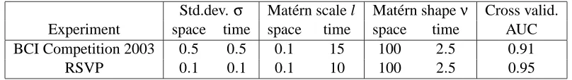
Std.dev.σ Mat´ern scale l Mat´ern shapeν Cross valid.
Experiment space time space time space time AUC
BCI Competition 2003 0.5 0.5 0.1 15 100 2.5 0.91
RSVP 0.1 0.1 0.1 10 100 2.5 0.95
Table 1: The parameter values for the Mat´ern covariance function (6) are summarized in this table. The values were found by optimizing AUC using five-fold cross validation. Note that the scale parameter l is defined spatially on a head with unitless radius of 0.5, and defined
temporally in terms of samples (l =15 corresponds to 150ms for the BCI Competition
data, while l=10 corresponds to 78ms for the RSVP data).
curve (‘AUC’, see Fawcett, 2003) using five-fold cross validation. The resulting set of parameter values are summarized in the first row of Table 1, and the resulting number of components was
R=1.
Benchmark performance was measured on the test set which had not been used during either training or cross validation. The number of misclassified trials in the test set was 21 which places our method on a new third place given the result of the competition which can be found online at http://ida.first.fraunhofer.de/projects/bci/competition_ii/results/index.html (Blankertz et al., 2004). These benchmark results indicate that classification of single-trial EEG is indeed a hard problem. Hence, our method works as a classifier producing a state-of-the art result in this hard data set. We estimated the SNR of this discriminating signal to SNR≈10 log10(Pk/P⊥) = −43dB, where Pkis the power of the projected signal, and P⊥is the power in the orthogonal space. The achieved classification performance supports the validity of the bilinear weight space factoriza-tion in EEG.
4.2 Experiment II: Bilinear Discriminant Component Analysis of Real EEG
We applied the BDCA method in real EEG data which was recorded while the human subjects were stimulated with a sequence of images presented at a rate of ten images per second. Each subject attended to a computer monitor where most of the images where ‘distractors’, that is, of no particular interest. Rare but anticipated ‘target’ images were to be detected by the subject. This paradigm is also known as Rapid Serial Visual Presentation (RSVP) (Thorpe et al., 1996; Gerson et al., 2005). In this experiment the subject was instructed to omit any overt response to the targets but simply note its occurrence. The images used here were identical to those of Gerson et al. (2005). Sixty-four EEG channels were recorded at 2048Hz, re-referenced to average reference (one channel removed to obtain full row-rank data), filtered (for anti-aliasing) and downsampled to
128Hz sampling rate, and filtered again with a pass-band between 0.5Hz and 50Hz. All filtering
was applied forwards and backwards in time to avoid introducing group delay. Trial matrices of dimension(D,T) = (64,64)were extracted by epoching (500ms per epoch) the data in alignment
with image stimulus. The number of recorded target/distractor trials was roughly 60/3000 for
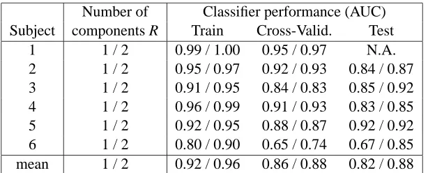
Number of Classifier performance (AUC)
Subject components R Train Cross-Valid. Test
1 1 / 2 0.99 / 1.00 0.95 / 0.97 N.A.
2 1 / 2 0.95 / 0.97 0.92 / 0.93 0.84 / 0.87
3 1 / 2 0.91 / 0.95 0.84 / 0.83 0.85 / 0.92
4 1 / 2 0.96 / 0.99 0.91 / 0.93 0.83 / 0.85
5 1 / 2 0.92 / 0.95 0.88 / 0.87 0.92 / 0.92
6 1 / 2 0.80 / 0.90 0.65 / 0.74 0.67 / 0.85
mean 1 / 2 0.92 / 0.96 0.86 / 0.88 0.82 / 0.88
Table 2: Summary of classification performance of classifiers for all subjects. Classifiers with two components generally perform better than single-component classifiers in both cross-validation and test.
4.2.1 TRAINING ANDRESULTS
We tuned the parameters using cross validation on the training set from a single subject, again using
R=1 and assuming standard electrode coordinates c.f. Section 4.1.1. The resulting set of parameter values are summarized in the second row of Table 1. For this subject, the cross validation AUC was 0.95, and corresponded to roughly 0.11 false positive rate and 0.89 true positive rate, indicating that the algorithm was successful in estimating a discriminating direction which was highly relevant for the experimental task. This finding underlines the usefulness of the method as a single-trial classifier for EEG.
Next, we trained classifiers for all subjects keeping the parameters fixed to the values in Table 1. The training, cross-validated, and test performances are reported in Table 2. In general the two-component classifiers performed slightly better than the single-two-component classifiers.
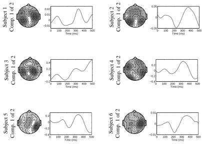
The G matrices (one for each subject) were estimated using the algorithm in Appendix B. Fig-ure 1 shows a single BDCA component for each subject. Clearly, there are inter-subject variability in the spatial topographies and in the temporal profiles, however, all temporal profiles exhibit positive peaks at around 125ms and 300ms after target stimulus, and negative peak at around 200ms. The peak at 300ms in the temporal profile is in agreement with the conventional P300 which is typically observed with a rare target stimulus (Gerson et al., 2005; Parra et al., 2005). The early peak (here around 125ms) had likewise been reported previously for the RSVP paradigm (Thorpe et al., 1996). The spatial topographies shown in Figure 1 are rather complex. This may simply represent noise, but it is also possible that BDCA, using additional trials and R>2, could decompose the complex rank-one patterns into more than two components with localized, that is, ‘simpler’, topography.
Subject 1 Comp. 1 of 2
0 100 200 300 400 500 −0.01 0 0.01 0.02 Time (ms) Subject 2 Comp. 1 of 2
0 100 200 300 400 500 −0.05 0 0.05 Time (ms) Subject 3 Comp. 1 of 2
0 100 200 300 400 500 −0.2 0 0.2 0.4 Time (ms) Subject 4 Comp. 1 of 2
0 100 200 300 400 500 −0.4 −0.2 0 0.2 Time (ms) Subject 5 Comp. 1 of 2
0 100 200 300 400 500 −0.4 −0.2 0 0.2 Time (ms) Subject 6 Comp. 1 of 2
0 100 200 300 400 500 −0.01
0 0.01
Time (ms)
Figure 1: For each subject, one of the (spatial) ak vectors is shown topographically on a cartoon
head, and the corresponding (temporal) bk vector is shown right next to it. The sign
ambiguity between component topographies and time courses has been set so that the P300 peak has a positive projection to the center in the back of the cartoon head. All temporal profiles exhibit positive peaks at around 100ms and 350ms (P300) after target stimulus, and negative peak at around 200ms.
Subject 4 Comp. 2 of 2
0 100 200 300 400 500 −0.02 0 0.02 Time (ms) Subject 6 Comp. 2 of 2
0 100 200 300 400 500 0
10 20x 10
−4
Time (ms)
for Subject 4, and 0.87 AUC for subject 6 which indicated that the newly identified components were indeed associated with target detection.
Finally we would like to point out that the resulting smoothness (e.g., the time courses in Fig-ure 1) is not only affected by the choice of regularization parameters but also by the data and the number of trials. If more data is available that supports a deviation from the prior smoothness assumption the resulting time courses can and will be more punctuated in time.
5. Conclusion and Discussion
Bilinear Discriminant Analysis (BLDA) can give better classification performance in situations where a bilinear decomposition of the parameter matrix can be assumed as in (5). Such parameter matrix decompositions might prove reasonable in situations were component analysis according to model (2) is meaningful. A ‘component’ in this model is considered to be all the activity that can be associated with a common time course. One such component contributes to a rank-one subspace in data Xn. If separate spatial distributions have separate time courses the model assumes that these
contribution add up linearly. For instance, when applying this on fMRI data the implicit assumption would be that the BOLD signal originating from different neuronal populations is additive.
We presented a method for BLDA which allows smoothness regularization for better general-ization performance in data sets with limited examples. This step was motivated by application to functional brain imaging were the number of examples is typically very limited compared to the data space dimensionality. The proposed BLDA method was verified in a benchmark data set, and the results were highly competitive, putting the new method on a place between the official second and third places of the competition.
We showed that BLDA can yield a data subspace factorization which makes it a useful tool for supervised extraction of components as opposed to simply a tool for classifying data matrices. We identified some essential ambiguities in such supervised subspace component decomposition and proposed to resolve them by assuming independence across the labeled mode (i.e., across trials in the EEG examples). The new method (BDCA: Bilinear Discriminant Component Analysis) thus combines BLDA with ICA and was applied to real EEG data from six human subjects. The results were in agreement with literature on the given experiment. Furthermore, a hypothesis was generated due to some components that had not been reported previously.
Model selections (i.e., finding the number of components) was based solely on classification. Then, given the optimal number of components, ICA was performed as a separate step. Future work will consider the combined likelihood to select a model that optimizes simultaneously both discrimination and independence.
Acknowledgments
The EEG topographies in this paper were plotted using the Matlab toolbox “EEGLAB” (Delorme and Makeig, 2004).
Appendix A. Maximum-Likelihood Estimation of U and V
Parameter estimation in a Logistic Regression model is often done though iterative maximum like-lihood estimation using Newton-Raphson updates (McCulloch and Searle, 2001). In line with tra-ditional Logistic Regression we assume the labels independent and Bernoulli distributed. The log likelihood is then given by
l(w0,{ur,vr}) = N
∑
n=1
yn(w0+ R
∑
r=1
uTrXnvr)−log(1+ew0+∑
R
r=1uTrXnvr) (10)
where ynis the nth label, uris the rth column vector of U, vris the rth column vector of V, and w0
is a scalar that enables a possible activation offset in the logistic function. Define
π(Xn)≡E[yn] = 1
1+e−(w0+∑Rr=1uTrXnvr).
hen, the gradient of (10) is given by
∂l
∂w0
=
∑
n
yn−π(Xn),
∂l
∂ur
=
∑
n
Xnvr[yn−π(Xn)],
∂l
∂vT r
=
∑
n
uTrXn[yn−π(Xn)],
and the Hessian matrix entries are given by
∂2l
∂w0∂w0
=−
∑
n
π(Xn)[1−π(Xn)],
∂2l
∂w0∂ur
=−
∑
n
Xnvrπ(Xn)[1−π(Xn)],
∂2l
∂w0∂vTr
=−
∑
n
uTrXnπ(Xn)[1−π(Xn)],
∂2l
∂ur∂(uk0)j =−
∑
n Xnvr(Xnvk0)jπ(Xn)[1−π(Xn)],
∂2l
∂vT r∂(vk0)j
=−
∑
n
∂2l
∂ur∂(vTk0)j
=
∑
n
δk,k0(Xn): j[yn−π(Xn)]−Xnvr(uTk0Xn)jπ(Xn)[1−π(Xn)],
where δk,k0 =1 for k=k0and zero otherwise. We provide no guarantee that the Hessian matrix will be definite, and in our experiments in this paper we obtain ML estimates using the so-called ‘Damped Newton’ optimization scheme which will take regularized Newton steps using adaptive regularization of the Hessian matrix (Bishop, 1996; Nielsen, 2005).
A.1 Smoothness Regularization with Gaussian Processes
The log posterior is equal to the log likelihood plus evaluation of the log prior, that is,
log p(w0,{ur,vr}|X) =l(w0,{ur,vr}) +log p(w0,{ur,vr})−log p(X)
where X denotes data in all the trials available. Here we consider the maximum of the posterior (MAP) estimate, that is,
(w0,{ur,vr})MAP=arg max w0,{ur,vr}
l(w0,{ur,vr}) +log p(w0,{ur,vr})
with independent priors
log p(w0,{ur,vr}) =log p(w0) +
∑
rlog p(ur) +
∑
rlog p(vr). (11)
For iterative MAP estimation, the terms for the Gaussian prior, to be inserted in (11), are (here shown for ur)
log p(ur) =−dim ur
2 log(2π)− 1
2log(det K)− 1 2u
T rK−1ur
where dim ur=D (or likewise dim vr=T or dim w0=1) (see also Rasmussen and Williams, 2006).
The extra terms, to be added to the ML terms, are; for the gradient
∂log p(ur)
∂ur
=−K−1ur
and for the Hessian
∂2log p(u r)
∂ur∂(ur)j
=−K−1ej
where ejis the jth unit vector. These expressions (and similar for w0and vr) thus augment the terms
in the maximum likelihood algorithm above.
Appendix B. Equations for Maximum-Likelihood Estimation of G
The log likelihood is given by
log p(Xn|VGˆ −1,UGˆ T) =− N
2 log det[A
TA] +
∑
nlog p(ˆsn)
see also Dyrholm et al. (2006) and http://www.imm.dtu.dk/˜mad/papers/madrix.pdf. We
(1995), which is appropriate for super-Gaussian independent activations (see also Lee et al., 1999). This choice however might not fit the scaling of the data very well so we parameterize the activation pdf and rewrite the likelihood
log p(Xn|VGˆ −1,UGˆ T,α) =− N
2log det[A
TA] +
∑
nlog p(ˆzn/α2)
where ˆzk(n) = (sˆk(n)−E[sˆk(n)])/
p
var[sˆk(n)]. Again, we use Damped Newton optimization which will take regularized Newton steps using adaptive regularization of the Hessian matrix (Bishop, 1996; Nielsen, 2005). We do not actually compute the Hessian but use the outer product approxi-mation to the Hessian given by averaging gradient products across trials (see also Bishop, 1996).
The gradient of the determinant term of the log likelihood, with respect to G, is given by
∂−N
2log det[ATA]
∂(G)i j =−N Trace
(
(A+)T
∂
A
∂(G)i j
T)
where
∂A
∂(G)i j
=−V(G−1eieTjG−1)|⊗|UGT+VG−1|⊗|UejeTi
The gradient of the sum term of the log likelihood, with respect to G, is given by
∂log p(A+vec(Xn)/α2)
∂(G)i j = [ψ(ˆsn/α
2)]T ∂ˆsn
∂(G)i j/α 2
where
ψ(·) = p0(·)
p(·) =−tanh(·)
and
∂ˆsn
∂(G)i j =
∂
(ATA)−1
∂(G)i j
AT+ (ATA)−1 ∂A T
∂(G)i j
vec(Xn)
where
∂(ATA)−1
∂(G)i j
=−(ATA)−1Trace
∂
AT
∂(G)i j
A+AT ∂A
∂(G)i j
(ATA)−1.
References
A. H. Andersen and W. S. Rayens. Structure-seeking multilinear methods for the analysis of fMRI data. Neuroimage, 22(2):728–39, 2004.
C.F. Beckmann and S.M. Smith. Tensorial extensions of independent component analysis for group fMRI data analysis. NeuroImage, 25(1):294–311, 2005.
A. J. Bell and T. J. Sejnowski. An information-maximization approach to blind separation and blind deconvolution. Neural Computation, 7(6):1129–1159, 1995.
B. Blankertz, G. Curio, and K.-R. M ¨uller. Classifying single trial EEG: Towards brain computer interfacing. In T. G. Diettrich, S. Becker, and Z. Ghahramani, editors, Advances in Neural Inf.
Proc. Systems 14 (NIPS 01), 2002.
B. Blankertz, K.-R. M ¨uller, G. Curio, T.M. Vaughan, G. Schalk, J.R. Wolpaw, A. Schlogl, C. Ne-uper, G. Pfurtscheller, T. Hinterberger, M. Schroder, and N. Birbaumer. The BCI competition 2003: progress and perspectives in detection and discrimination of EEG single trials. Biomedical
Engineering, IEEE Transactions on, 51(6):1044–1051, 2004.
R. Bro. Multi-way Analysis in the Food Industry. PhD thesis, Royal Veterinary and Agricultural University, Denmark, 1998.
E. T. Bullmore, S. Rabe-Hesketh, R. G. Morris, S. C. Williams, L. Gregory, J. A. Gray, and M. J. Brammer. Functional magnetic resonance image analysis of a large-scale neurocognitive network.
Neuroimage, 4(1):16–33, 1996.
V. Calhoun, T. Adali, G. Pearlson, and J. Pekar. Spatial and temporal independent component analysis of functional MRI data containing a pair of task-related waveforms. Hum Brain Mapp, 13:43, 2001.
L. De Lathauwer and J. Vandewalle. Dimensionality reduction in higher-order signal processing and rank-(R1,R2, ...,RN) reduction in multilinear algebra. Lin. Alg. Appl., 391:31–55, 2004.
A. Delorme and S. Makeig. Eeglab: an open source toolbox for analysis of single-trial eeg dynamics including independent component analysis. J Neurosci Methods, 134(1):9–21, 2004.
M. Dyrholm, S. Makeig, and L. K. Hansen. Model selection for convolutive ICA with an application to spatio-temporal analysis of EEG. Neural Computation, 2006.
M. Dyrholm and L. C. Parra. Smooth bilinear classification of EEG. In Proceedings of the IEEE
2006 International Conference of the Engineering in Medicine and Biology Society, 2006.
T. Fawcett. ROC graphs: Notes and practical considerations for data mining researchers. Technical report, HPL-2003-4. HP Laboratories, Palo Alto, CA, USA., 2003.
A.D. Gerson, L.C. Parra, and P. Sajda. Cortical origins of response time variability during rapid discrimination of visual objects. NeuroImage, 28(2):326–341, 2005.
R. A. Harshman. Foundations of the PARAFAC procedure: Models and conditions for an ‘explana-tory’ multi-modal factor analysis. UCLA Working Papers in Phonetics, 16, 1970.
J. B. Kruskal. Three-way arrays: Rank and uniqueness of trilinear decompositions, with application to arithmetic complexity and statistics. Linear Algebra and its Applications, 18:95–138, 1977.
T.-W. Lee, M. Girolami, and T. J. Sejnowski. Independent component analysis using an extended infomax algorithm for mixed sub-gaussian and super-gaussian sources. Neural Computation, 11 (2):417–441, 1999.
S. Makeig, A. J. Bell, T.-P. Jung, and T. J. Sejnowski. Independent component analysis of electroen-cephalographic data. In M. Mozer and M. Hasselmo, editors, Advances in Neural Information
E. Martinez-Montes, P. A. Valdes-Sosa, F. Miwakeichi, R. I. Goldman, and M. S. Cohen. Concurrent EEG/fMRI analysis by multiway Partial Least Squares. NeuroImage, 22(3):1023–1034, 2004.
C. E. McCulloch and S. R. Searle. Generalized, Linear, and Mixed Models. Wiley, 2001.
F. Miwakeichi, E. Martinez-Montes, P. A. Valdes-Sosa, N. Nishiyama, H. Mizuhara, and Y. Ya-maguchi. Decomposing EEG data into space-time-frequency components using parallel factor analysis. Neuroimage, 22(3):1035–45, 2004.
N. Mørch, L. Hansen, S. Strother, C. Svarer, D. Rottenberg, and B. Lautrup. Nonlinear vs. linear models in functional neuroimaging: Learning curves and generalization crossover. In
Proceed-ings of the 15th international conference on information processing in medical imaging, volume
1230 of Lecture Notes in Computer Science, pages 259–270. Springer, 1997.
J. M¨ocks. Decomposing event-related potentials: A new topographic components model. Biol
Psychol, 26(1-3):199–215, 1988.
M. Mørup, L. K. Hansen, C. S. Hermann, J. Parnas, and S. M. Arnfred. Parallel factor analysis as an exploratory tool for wavelet transformed event-related EEG. NeuroImage, 29(3):938–947, feb 2006.
H. B. Nielsen. IMMOPTIBOX. General optimization software available athttp://www.imm.dtu.
dk/˜hbn/immoptibox/, 2005.
L. Parra, C. Spence, A. Gerson, and P. Sajda. Recipes for the linear analysis of EEG. NeuroImage, 28:326–341, 2005.
W. D. Penny, N. J. Trujillo-Barreto, and K. J. Friston. Bayesian fMRI time series analysis with spatial priors. NeuroImage, 24:350–362, 2005.
C. E. Rasmussen and C. K. I. Williams. Gaussian Processes for Machine Learning. 272, The MIT Press, Cambridge, Massachusetts, 2006.
Y. Sakaguchi, S. Ozawa, and M. Kotani. Feature extraction using supervised independent com-ponent analysis by maximizing class distance. In Proc. of Int. Conf. on Neural Information
Processing, volume 5, pages 2502–2506, 2002.
K. C. Squires, E. Donchin, R. I. Herning, and G. McCarthy. On the influence of task relevance and stimulus probability on event-related-potential components. Electroencephalogr Clin
Neu-rophysiol, 1977.
S. Thorpe, D. Fize, and C. Marlot. Speed of processing in the human visual system. Nature, 381 (6582):520–2, 1996.
M. Visani, C. Garcia, Jolion, and J.-M. Normalized radial basis function networks and bilinear discriminant analysis for face recognition. In Proceedings. IEEE Conference on Advanced Video
and Signal Based Surveillance, pages 342–47, 2005.