QP Algorithms with Guaranteed Accuracy and Run Time
for Support Vector Machines
Don Hush [email protected]
Patrick Kelly [email protected]
Clint Scovel [email protected]
Ingo Steinwart [email protected]
Modeling, Algorithms and Informatics Group, CCS-3, MS B265 Los Alamos National Laboratory
Los Alamos, NM 87545 USA
Editor: Bernhard Sch¨olkopf
Abstract
We describe polynomial–time algorithms that produce approximate solutions with guaranteed ac-curacy for a class of QP problems that are used in the design of support vector machine classifiers. These algorithms employ a two–stage process where the first stage produces an approximate so-lution to a dual QP problem and the second stage maps this approximate dual soso-lution to an ap-proximate primal solution. For the second stage we describe an O(n log n)algorithm that maps an approximate dual solution with accuracy(2√2Kn+8
√ λ)−2λε2
pto an approximate primal solution with accuracyεpwhere n is the number of data samples, Knis the maximum kernel value over the data andλ>0 is the SVM regularization parameter. For the first stage we present new results for decomposition algorithms and describe new decomposition algorithms with guaranteed accu-racy and run time. In particular, forτ–rate certifying decomposition algorithms we establish the
optimality ofτ=1/(n−1). In addition we extend the recentτ=1/(n−1)algorithm of Simon (2004) to form two new composite algorithms that also achieve theτ=1/(n−1)iteration bound of List and Simon (2005), but yield faster run times in practice. We also exploit theτ–rate certifying property of these algorithms to produce new stopping rules that are computationally efficient and that guarantee a specified accuracy for the approximate dual solution. Furthermore, for the dual QP problem corresponding to the standard classification problem we describe operational conditions for which the Simon and composite algorithms possess an upper bound of O(n)on the number of iterations. For this same problem we also describe general conditions for which a matching lower bound exists for any decomposition algorithm that uses working sets of size 2. For the Simon and composite algorithms we also establish an O(n2)bound on the overall run time for the first stage. Combining the first and second stages gives an overall run time of O(n2(c
k+1))where ckis an upper bound on the computation to perform a kernel evaluation. Pseudocode is presented for a complete algorithm that inputs an accuracyεpand produces an approximate solution that satisfies this accuracy in low order polynomial time. Experiments are included to illustrate the new stopping rules and to compare the Simon and composite decomposition algorithms.
1. Introduction
Solving a quadratic programming (QP) problem is a major component of the support vector machine (SVM) training process. In practice it is common to employ algorithms that produce approximate solutions. This introduces a trade-off between computation and accuracy that has not been thor-oughly explored. The accuracy, as measured by the difference between the criterion value of the approximate solution and the optimal criterion value, is important for learning because it has a di-rect influence on the generalization error. For example, since the optimal criterion value plays a key role in establishing the SVM performance bounds in (Steinwart and Scovel, 2004, 2005; Scovel et al., 2005b) the influence of the accuracy can be seen directly through the proofs of these bounds. Since the primal QP problem can be prohibitively large and its Wolfe dual QP problem is consider-ably smaller it is common to employ a two–stage training process where the first stage produces an approximate solution to the dual QP problem and the second stage maps this approximate dual so-lution to an approximate primal soso-lution. Existing algorithms for the first stage often allow the user to trade accuracy and computation for the dual QP problem through the choice of a tolerance value that determines when to stop the algorithm, but it is not known how to choose this value to achieve a desired accuracy or run time. Furthermore existing algorithms for the second stage have been developed largely without concern for accuracy and therefore little is known about the accuracy of the approximate primal solutions they produce. In this paper we describe algorithms that accept the accuracyεp of the primal QP problem as an input and are guaranteed to produce an approximate
solution that satisfies this accuracy in low order polynomial time. To our knowledge these are the first algorithms of this type for SVMs. In addition our run time analysis reveals the effect of the accuracy on the run time, thereby allowing the user to make an informed decision regarding the trade–off between computation and accuracy.
Algorithmic strategies for the dual QP problem must address the fact that when the number of data samples n is large the storage requirements for the kernel matrix can be excessive. This bar-rier can be overcome by invoking algorithmic strategies that solve a large QP problem by solving a sequence of smaller QP problems where each of the smaller QP problems is obtained by fixing a subset of the variables and optimizing with respect to the remaining variables. Algorithmic strate-gies that solve a QP problem in this way are called decomposition algorithms and a number have been developed for dual QP problems: (Balcazar et al., 2001; Chen et al., 2005, 2006; Cristian-ini and Shawe-Taylor, 2000; Hsu and Lin, 2002; Hush and Scovel, 2003; Joachims, 1998; Keerthi et al., 2000, 2001; Laskov, 2002; Liao et al., 2002; List and Simon, 2004, 2005; Mangasarian and Musicant, 1999, 2001; Osuna et al., 1997; Platt, 1998; Simon, 2004; Vapnik, 1998).
The key to developing a successful decomposition algorithm is in the method used to determine the working sets, which are the subsets of variables to be optimized at each iteration. To guaran-tee stepwise improvement each working set must contain a certifying pair (Definition 3 below). Stronger conditions are required to guarantee convergence: (Chang et al., 2000; Chen et al., 2006; Hush and Scovel, 2003; Lin, 2001a,b; List and Simon, 2004) and even stronger conditions appear necessary to guarantee rates of convergence: (Balcazar et al., 2001; Hush and Scovel, 2003; Lin, 2001a). Indeed, although numerous decomposition algorithms have been proposed few are known to possess polynomial run time bounds. Empirical studies have estimated the run time of some common decomposition algorithms to be proportional to npwhere p varies from approximately 1.7
pre-dicting the run time for future problem instances. In addition these particular studies do not appear to be calibrated with respect to the accuracy of the final criterion value and so their relevance to the framework considered here is not clear. Lin (2001a) performs a convergence rate analysis that may eventually be used to establish run time bounds for a popular decomposition algorithm, but these results hold under rather restrictive assumptions and more work is needed before the tightness and utility of these bounds is known (a more recent version of this analysis can be found in (Chen et al., 2006)). Balcazar et al. (2001) present a randomized decomposition algorithm whose expected run time is O (n+r(k2d2))kd log nwhere n is the number of samples, d is the dimension of the input space, 1≤k≤n is a data dependent parameter and r(k2d2)is the run time required to solve the dual QP problem overk2d2samples. This algorithm is very attractive whenk2d2≪n, but in
practice the value ofkis unknown and it may be large when the Bayes error is not close to zero. Hush and Scovel (2003) define a class of rate certifying algorithms and describe an example al-gorithm that uses O
Knn5log n
ε
computation to reach an approximate dual solution with accuracy
ε, where Kn is the maximum value of the kernel matrix. Recently Simon (2004) introduced a new
rate certifying algorithm which can be shown, using the results in (List and Simon, 2005), to use
OnKnλε +n2logλKnncomputation to reach an approximate dual solution with accuracyε, where
λ>0 is the SVM regularization parameter. In this paper we combine Simon’s algorithm with the popular Generalized SMO algorithm of Keerthi et al. (2001) to obtain a composite algorithm that possesses the same computation bound as Simon’s algorithm, but appears to use far less computa-tion in practice (as illustrated in our experiments). We also extend this approach to form a second
composite algorithm with similar properties. In addition we introduce operational assumptions on Knand the choice ofλandεthat yield a simpler computation bound of O(n2)for these algorithms.
Finally to guarantee that actual implementations of these algorithms produce approximate solutions with accuracyεwe introduce two new stopping rules that terminate the algorithms when an adap-tively computed upper bound on the accuracy falls belowε.
The second stage of the design process maps an approximate dual solution to an approximate primal solution. In particular this stage determines how the approximate dual solution is used to form the normal vector and offset parameter for the SVM classifier. It is common practice to use the approximate dual solution as coefficients in the linear expansion of the data that forms the nor-mal vector, and then use a heuristic based on approximate satisfaction of the Karush-Kuhn-Tucker (KKT) optimality conditions to choose the offset parameter. This approach is simple and compu-tationally efficient, but it produces an approximate primal solution whose accuracy is unknown. In this paper we take a different approach based on the work of Hush et al. (2005). This work studies the accuracy of the approximate primal solution as a function of the accuracy of the ap-proximate dual solution and the map from apap-proximate dual to apap-proximate primal. In particular for the SVM problem it appears that choosing this map involves a trade–off between computation and accuracy. Here we employ a map described and analyzed in (Hush et al., 2005) that guarantees an accuracy ofεp for the primal QP problem when the dual QP problem is solved with accuracy
(2√2Kn+8 √
λ)−2λε2
p. This map resembles current practice in that it performs a direct substitution
of the approximate dual solution into a linear expansion for the normal vector, but differs in the way that it determines the offset parameter. We develop an O(n log n)algorithm that computes the offset parameter according to this map.
established in (Hush et al., 2005). Section 2 describes the SVM formulation, presents algorithms for the first and second stages, and provides theorems that characterize the accuracy and run time for these algorithms. Section 3 then determines specific run time bounds for decomposition algorithms applied to the standard classification problem and the density level detection problem. Section 4 describes experiments that illustrate the new stopping rules and compare the run time of different decomposition algorithms. Section 5 provides a summary of results and establishes an overall run time bound. A complete algorithm that computes anεp–optimal solution to the primal QP problem
is provided by (Procedure 1, Section 2) and Procedures 3–8 in the appendix.
2. Definitions, Algorithms, and Main Theorems
Let X be a pattern space and k : X×X→Rbe a kernel function with Hilbert space H and feature mapφ: X→H so that k(x1,x2) =φ(x1)·φ(x2),∀x1,x2∈X . Define Y :={−1,1}. Given a data set
((x1,y1), ...,(xn,yn))∈(X×Y)nthe primal QP problem that we consider takes the form
minψ,b,ξ λkψk2+∑n i=1uiξi
s.t. yi(φ(xi)·ψ+b)≥1−ξi ξi≥0, i=1,2, ...,n
(1)
whereλ>0, ui >0 and ∑iui =1. This form allows a different weight ui for each data sample.
Specific cases of interest include:
1. the L1–SVM for the standard supervised classification problem which sets ui =1/n, i=
1, ...,n,
2. the DLD–SVM for the density level detection problem described in (Steinwart et al., 2005) which sets
ui=
( 1
(1+ρ)n1, yi=1
ρ
(1+ρ)n−1, yi=−1
where n1is the number of samples distributed according to P1and assigned label y=1, n−1is
the number of samples distributed according to P−1and assigned label y=−1, h=dP1/dP−1
is the density function, andρ>0 defines theρ–level set{h>ρ}that we want to detect.
The dual QP problem is
maxa −12a·Qa+a·1
s.t. y·a=0
0≤ai≤ui i=1,2, ...,n.
(2)
where
Qi j=yiyjk(xi,xj)/2λ.
The change of variables defined by
αi:=yiai+li, li=
0 yi=1
ui yi=−1 (3)
gives the canonical dual QP problem
maxα −12α·Qα+α·w+w0
s.t. 1·α=c
0≤αi≤ui i=1,2, ...,n
where
Qi j=k(xi,xj)/2λ, c=l·1, w=Ql+y, w0=−l·y−
1
2l·Ql. (5)
We denote the canonical dual criterion by
R(α):=−1
2α·Qα+α·w+w0.
Note that this change of variables preserves the criterion value. Also note that the relation between
a and α is one–to–one. Most of our work is with the canonical dual because it simplifies the algorithms and their analysis.
We define the set ofε–optimal solutions of a constrained optimization problem as follows.
Definition 1 Let P be a constrained optimization problem with parameter spaceΘ, criterion func-tion G :Θ→R, feasible set ˜Θ⊆Θ of parameter values that satisfy the constraints, and optimal criterion value G∗(i.e. G∗=supθ∈Θ˜G(θ)for a maximization problem and G∗=infθ∈Θ˜G(θ)for a minimization problem). Then for anyε≥0 we define
O
ε(P):={θ∈Θ˜ :|G(θ)−G∗| ≤ε}to be the set ofε–optimal solutions for P.
We express upper and lower computation bounds using O(·)andΩ(·)notations defined by
O(g(n)) ={f(n):∃positive constants c and n0such that 0≤ f(n)≤cg(n)for all n≥n0}, Ω(g(n)) ={f(n):∃positive constants c and n0such that 0≤cg(n)≤ f(n)for all n≥n0}.
We now describe our algorithm for the primal QP problem. It computes an approximate canon-ical dual solution ˆα and then maps to an approximate primal solution(ψˆ,ˆb,ξˆ) using the map de-scribed in the following theorem. This theorem is derived from (Hush et al., 2005, Theorem 2 and Corollary 1) which is proved using the result in (Scovel et al., 2005a).
Theorem 2 Consider the primal QP problem PSV M in (1) withλ>0 and|φ(xi)|2≤K,i=1, ..,n, and its corresponding canonical dual QP problem DSV M in (4) with criterion R. Letεp>0, ε=
(2√2K+8√λ)−2λε2
pand suppose that ˆα∈
O
ε(DSV M)and R(αˆ)≥0. Ifˆ
ψ= 1 2λ
n
∑
i=1
(αˆi−li)φ(xi)
ˆ
ξi(b) =max(0,1−yi(ψˆ ·φ(xi) +b)), i=1, ..,n
and
ˆb∈arg min
n
∑
i=1 uiξˆi(b)
This theorem gives an expression for ˆψ that coincides with the standard practice of replacing an optimal dual solutionα∗ by an approximate dual solution ˆαin the expansion for the optimal nor-mal vector determined by the KKT conditions. The remaining variables ˆξand ˆb are obtained by substituting ˆψinto the primal optimization problem, optimizing with respect to the slack variableξ, and then minimizing with respect to b1. To guarantee an accuracyεp for the primal problem this
theorem stipulates that the value of the dual criterion at the approximate solution be non–negative and that the accuracy for the dual solution satisfy ε= (2√2K+8√λ)−2λε2
p. The first condition
is easily achieved by algorithms that start withα=l (so that the initial criterion value is 0) and
continually improve the criterion value at each iteration. We will guarantee the second condition by employing an appropriate stopping rule for the decomposition algorithm.
Procedure 1 shows the primal QP algorithm that produces an εp–optimal solution(αˆ,ˆb) that
defines the SVM classifier
sign
n
∑
i=1
ˆ
αi−l
2λ
k(xi,x) +ˆb !
.
This algorithm inputs a data set Tn= ((x1,y1), ...,(xn,yn)), a kernel function k, and parameter values λ, u andεp. Lines 3–6 produce an exact solution for the degenerate case where all the data samples
have the same label. The rest of the routine forms an instance of the canonical dual QP according to (5), setsεaccording to Theorem 2, setsα0=l so that R(α0) =0, uses the routineDecomposition
to compute anε–approximate canonical dual solution ˆα, and uses the routineOffsetto compute the offset parameter ˆb according to Theorem 2. The parameter g, which is defined in the next section, is a temporary value computed byDecomposition that allows a more efficient computation of ˆb byOffset. The next three sections provide algorithms and computational bounds for the routines
DecompositionandOffset.
Procedure 1 The algorithm for the primal QP problem.
1: PrimalQP(Tn,k,λ,u,εp)
2:
3: if (yi=y1,∀i) then
4: αˆ ←l, ˆb←y1
5: Return( ˆα,ˆb)
6: end if
7: Form canonical dual: Qi j←k(xi2,λxj), li←(1−2yi)ui, w←Ql+y, c←l·1
8: Compute Desired Accuracy of Dual:ε← λε
2
p
(2√2K+8√λ)2
9: Initialize canonical dual variable:α0←l
10: (αˆ,g)←Decomposition(Q,w,c,u,ε,α0)
11: ˆb←Offset(g,y,u)
12: Return( ˆα,ˆb)
2.1 Decomposition Algorithms
We begin with some background material that describes: optimality conditions for the canonical dual, a model decomposition algorithm, necessary and sufficient conditions for convergence to a
solution, and sufficient conditions for rates of convergence. In many cases this background material extends a well known result to the slightly more general case considered here where each component of u may have a different value.
Consider an instance of the canonical dual QP problem given by(Q,w,w0,c,u). Define the set
of feasible values
A
:={α:(0≤αi≤ui)and(α·1=c)},and the set of optimal solutions
A
∗:=arg maxα∈AR(α).
Also define the optimal criterion value R∗:=supα∈AR(α)and the gradient atα
g(α):=∇R(α) =−Qα+w. (6)
The optimality conditions established by Keerthi et al. (2001) take the form,
α∈
A
∗ ⇔ gj(α)≤gk(α)for all j :αj<uj,k :αk>0. (7)These conditions motivate the following definition from (Keerthi et al., 2001; Hush and Scovel, 2003).
Definition 3 A certifying pair (also called a violating pair) forα∈
A
is a pair of indices that witness the non–optimality ofα, i.e. it is a pair of indices j :αj<ujand k :αk>0 such that gj(α)>gk(α).Using the approach in (Hush and Scovel, 2003, Section 3) it can be shown that the requirement that working sets contain a certifying pair is both necessary and sufficient to obtain a stepwise improvement in the criterion value. Thus, since certifying pairs are defined in terms of the gradient component values it appears that the gradient plays an essential role in determining members of the working sets. To compute the gradient at each iteration using (6) requires O(n2) operations. However since decomposition algorithms compute a sequence of feasible points (αm)
m≥0 using
working sets of size p, the sparsity of(αm+1−αm)means that the update
g(αm+1) =g(αm)−Q(αm+1−αm) (8) requires only O(pn) operations. A model decomposition algorithm that uses this update is shown in Procedure 2. After computing an initial gradient vector this algorithm iterates the process of determining a working set, solving a QP problem restricted to this working set, updating the gradient vector, and testing a stopping condition.
The requirement that working sets contain a certifying pair is necessary but not sufficient to guarantee convergence to a solution (e.g. see the examples in Chen et al., 2006; Keerthi and Ong, 2000). However Lin (2002b) has shown that including a max–violating pair defined by
(j∗,k∗) : j∗∈arg max
i:αi<ui
gi(α), k∗∈arg min i:αi>0
gi(α) (9)
Procedure 2 A model decomposition algorithm for the canonical dual QP problem.
1: ModelDecomposition(Q,w,c,u,ε,α0)
2:
3: Compute initial gradient g0← −Qα0+w
4: m←0
5: repeat
6: Compute a working set Wm
7: Computeαm+1by solving the restricted QP determined byαmand Wm
8: Update the gradient: gm+1←gm−Q(αm+1−αm)
9: m←m+1
10: until (stopping condition is satisfied)
11: Return(αm,gm)
pair in each working set includes many popular algorithms (e.g. Chang and Lin, 2001; Joachims, 1998; Keerthi et al., 2001). Although asymptotic convergence to a solution is guaranteed for these algorithms, their convergence rate is unknown. In contrast we now describe algorithms based on alternative pair selection strategies that have the same O(n)computational requirements (once the gradient has been computed) but possess known rates of convergence to a solution.
Consider the model decomposition algorithm in Procedure 2. The run time of the main loop is the product of the number of iterations and the computation per iteration, and both of these depend heavily on the size of the working sets and how they are chosen. The smallest size that admits a convergent algorithm is 2 and many popular algorithms adopt this size. We refer to these as W2 decomposition algorithms. A potential disadvantage of this approach is that the number of iterations may be larger than it would be otherwise. On the other hand adopting working sets of size 2 allows us to solve each 2–variable QP problem in constant time (e.g. see Platt, 1998). In addition W2 decomposition algorithms require only O(n)computation to update the gradient and have the advantage that the overall algorithm can be quite simple (as demonstrated by the W2 max– violating pair algorithm). Furthermore adopting size 2 working sets will allow us to implement our new stopping rules in constant time. Thus, while most of the algorithms we describe below allow the working sets to be larger than 2, our experiments will be performed with their W2 variants.
In addition to their size, the content of the working sets has a significant impact on the run time through its influence on the convergence rate of the algorithm. Hush and Scovel (2003) prove that convergence rates can be guaranteed simply by including a rate certifying pair in each working set. Roughly speaking a rate certifying pair is a certifying pair that, when used as the working set, provides a sufficient stepwise improvement. To be more precise we start with the following definitions. Define a working set to be a subset of the index set of the components ofα, and let
W denote a working set of unspecified size and Wp denote a working set of size p. In particular Wn={1,2, ...,n}denotes the entire index set. The set of feasible solutions for the canonical dual
QP sub–problem defined by a feasible valueαand a working set W is defined
A
(α,W):={α´ ∈A
: ´αi=αi∀i∈/W}.Define
σ(α|W):= sup
´
α∈A(α,W)
to be the optimal value of the linear programming (LP) problem atα. The following definition is adapted from (Hush and Scovel, 2003).
Definition 4 For τ>0 an index pair W2 is called a τ–rate certifying pair for α if σ(α|W2)≥ τσ(α|Wn). A decomposition algorithm that includes a τ–rate certifying pair in the working set at every iteration is called aτ–rate certifying algorithm.
For aτ–rate certifying algorithm Hush and Scovel (2003) provide an upper bound on the number of iterations as a function of τ. An improved bound can be obtained as a special case of (List and Simon, 2005, Theorem 1). The next theorem provides a slightly different bound that does not depend on the size of the working sets and therefore slightly improves the bound obtained from (List and Simon, 2005, Theorem 1) when the size of the working sets is larger than 2.
Theorem 5 Consider the canonical dual QP problem in (4) with criterion function R and Gram matrix Q. Let L≥maxiQii and S≥maxiui. A τ–rate certifying algorithm that starts with α0 achieves R∗−R(αm)≤εafter⌈m´⌉iterations of the main loop where
´ m= 2 τln
R∗−R(α0) ε
+
, ε≥4LS
2 τ 2 τ 4LS2
τε −1+
ln
τ
(R∗−R(α0))
4LS2
+
, ε<4LS
2
τ ,
⌈θ⌉denotes the smallest integer greater than or equal toθ, and[θ]+=max(0,θ).
Chang et al. (2000) have shown that for every α∈
A
there exists a τ–rate certifying pair withτ≥1/n2. This result can be used to establish the existence of decomposition algorithms with polynomial run times. The first such algorithm was provided by Hush and Scovel (2003) where the rate certifying pairs satisfiedτ≥1/n2. However the valueτcan be improved and the bound on the number of iterations reduced if the rate certifying pairs are determined differently. Indeed List and Simon (2005) prove thatτ≥1/n for a max–lp2 pair
W2∗∈arg max
W2⊆Wn
σ(α|W2)
which is a pair with the maximum linear program value. The next theorem provides a slightly better result ofτ≥1/(n−1)for this pair and establishes the optimality of this bound2.
Theorem 6 Forα∈
A
max
W2⊆Wn
σ(α|W2)≥
σ(α|Wn) n−1 .
Furthermore, there exist problem instances for which there existα∈
A
such thatmax
W2⊆Wn
σ(α|W2) =
σ(α|Wn) n−1 .
2. This result provides a negligible improvement over theτ≥1/n result of List and Simon but is included here because it
Since a max–lp2 pair gives the largest value ofσ(α|W2)it follows from Definition 4 and
The-orem 6 that the largest single value ofτthat can be valid for all iterations of all problem instances is 1/(n−1). Thus a max–lp2 pair is optimal in that it achieves the minimum iteration bound in Theorem 5 with respect toτ. Furthermore Simon (2004) has introduced an algorithm for computing a max–lp2 pair that requires only O(n)computation and therefore coincides with the O(n) computa-tion required to perform the other steps in the main loop. However, in spite of the promise suggested by this analysis experimental results suggest that there is much room to improve the convergence rates achieved with max–lp2 pairs (e.g. see Section 4). The result below provides a simple way to determine pair selection methods whose convergence rates are at least as good as those guaranteed by the max–lp2 pair method and possibly much better. This result is stated as a corollary since it follows trivially from the proof of Theorem 5.
Corollary 7 LetDECOMPbe a realization of the model decomposition algorithm for the canonical dual QP in Procedure 2 and let (αm) represent a sequence of feasible points produced by this algorithm. At each iteration m let ´W2m be a τ–rate certifying pair and let ´αm+1 be the feasible point determined by solving the restricted QP determined byαm and ´W2m. If for every m≥0 the
stepwise improvement satisfies R(αm+1)−R(αm)≥R(α´m+1)−R(αm) then DECOMP will achieve R∗−R(αm)≤εafter⌈m´⌉iterations of the main loop where ´m is given by Theorem 5.
This theorem implies that any pair whose stepwise improvement is at least as good as that produced by a max–lp2 pair yields a decomposition algorithm that inherits the iteration bound in Theorem 5 withτ=1/(n−1). An obvious example is a max–qp2 pair, which is a pair with the
largest stepwise improvement. However since determining such a pair may require substantial
computation we seek alternatives. In particular Simon’s algorithm visits several good candidate pairs in its search for a max–lp2 pair and can therefore be easily extended to form an alternative pair selection algorithm that is computationally efficient and satisfies this stepwise improvement property. To see this we start with a description of Simon’s algorithm.
First note that when searching for a max–lp2 pair it is sufficient to consider only pairs (j,k) where gj(α)>gk(α). For such a pair it is easy to show that (e.g. see the proof of Theorem 6)
σ(α|{j,k}) =min(uj−αj,αk)(gj(α)−gk(α)) =∆jk(gj(α)−gk(α)) (10)
where ujis the upper bound onαj specified in (4) and∆jk:=min(uj−αj,αk). The key to Simon’s
algorithm is the recognition that among the O(n2) index pairs there are at most 2n distinct values for∆:
u1−α1, α1,u1−α2,α2, ..., un−αn,αn. (11)
Consider searching this list of values for one that corresponds to a maximum value ofσ. For an entry of the form uj−αj for some j, an index k that maximizesσ(α|{j,k})satisfies
k ∈ arg max
l:αl≥uj−αj
(gj(α)−gl(α)) = arg min l:αl≥uj−αj
gl(α).
Similarly for an entry of the formαk for some k, an index j that maximizesσ(α|{j,k})satisfies
j ∈ arg max
l:ul−αl≥αk
(gl(α)−gk(α)) = arg max l:ul−αl≥αk
gl(α).
value for entries of the formαkas we go. Then as we visit each entry in the list the index pair that
maximizesσcan be computed in constant time. Thus a max–lp2 pair can be determined in one pass through the list. A closer examination reveals that only the nonzero values at the front of the list need to be scanned, since entries with zero values cannot form a certifying pair (i.e. they correspond to pairs for which there is no feasible direction for improvement). In addition, since nonzero entries of the form uj−αjcorrespond to components j whereαj <uj, and nonzero entries of the formαk
correspond to components k whereαk>0, once the scan reaches the last nonzero entry in the list the
indices of the maximum and minimum gradient component values correspond to a max–violating pair. Pseudocode for this algorithm is shown in Procedure 4 in Appendix 6. This algorithm requires that the ordered list of values be updated at each iteration. If the entries are stored in a linear array this can be accomplished in O(pn)time by a simple search and insert algorithm, where p is the size of the working set. However, with the appropriate data structure (e.g. a red–black tree) this list can be updated in O(p log n)time. In this case the size of the working sets must satisfy p=O(n/log n) to guarantee an O(n)run time for the main loop.
Simon’s algorithm computes both a max–lp2 pair and a max–violating pair at essentially the same cost. In addition the stepwise improvement for an individual pair can be computed in constant time. Indeed with W2m={j,k}and g(αm
j)≥g(αmk)the stepwise improvementδmR takes the form
δm
R =
(
∆δg−∆2q/2, δg>q∆
δ2
g
2q, otherwise
(12)
whereδg=g(αmj)−g(αmk), q=Qj j+Qkk−2Qjk and∆=min uj−αmj,αmk
. Thus we can effi-ciently compute and compare the stepwise improvements of the max–violating and max–lp2 pairs and choose the one with the largest improvement. We call this the Composite–I pair selection method. It adds a negligible amount of computation to the main loop and its stepwise improvement cannot be worse than either the max–violating pair or max–lp2 algorithm alone. We can extend this idea further by computing the stepwise improvement for all certifying pairs visited by Simon’s algorithm and then choosing the best. We call this the Composite–II pair selection method. This methods adds a non–negligible amount of computation to the main loop, but may provide even bet-ter stepwise updates. It is worth mentioning that other methods have been recently introduced which examine a subset of pairs and choose the one with the largest stepwise improvement (e.g. see Fan et al., 2005; Lai et al., 2003). The methods described here are different in that they are designed specifically to satisfy the condition in Corollary 7.
We have described four pair selection methods; max–lp2, Composite–I (best of max–violating and max–lp2), Composite–II (best of certifying pairs visited by Simon’s algorithm), and max–qp2 (largest stepwise improvement) which all yield decomposition algorithms that satisfy the iteration bound in Theorem 5 withτ=1/(n−1), but whose actual computational requirements on a specific problem may be quite different. In Section 4 we perform experiments to investigate the actual computational requirements for these methods.
2.2 Stopping Rules
the stopping rule: stop at the first iteration ´m where
gj∗(αm´)−gk∗(αm´)≤tol (13)
where tol >0 is a user defined parameter. This stopping rule is employed by many existing de-composition algorithms (e.g. see Chang and Lin, 2001; Chen et al., 2006; Keerthi et al., 2001; Lin, 2002a) and is especially attractive for max–violating pair algorithms since the rule can be computed in constant time once a max–violating pair has been computed. Lin (2002a) justifies this rule by proving that the gap gj∗(αm)−gk∗(αm)converges to zero asymptotically for the sequence of
fea-sible points generated by a particular class of decomposition algorithms. In addition Keerthi and Gilbert (2002) prove that (13) is satisfied in a finite number of steps for a specific decomposition algorithm. However the efficacy of this stopping rule is not yet fully understood. In particular we do not know the relation between this rule and the accuracy of the approximate solution it produces, and we do not know the convergence rate properties of the sequence(gj∗(αm)−gk∗(αm))on which
the rule is based. In contrast we now introduce new stopping rules which guarantee a specified ac-curacy for the approximate solutions they produce, and whose convergence rate properties are well understood. In addition we will show that these new stopping rules can be computed in constant time when coupled with the pair selection strategies in the previous section.
The simplest stopping rule that guarantees anε–optimal solution for aτ–rate certifying algo-rithm is to stop after ´m iterations where ´m is given by Theorem 5 with R∗−R(α0)replaced by a
suitable upper bound (e.g. 1). We call this Stopping Rule 0. However the bound in Theorem 5 is conservative. For a typical problem instance the algorithm may reach the accuracyεin far fewer iterations. We introduce stopping rules that are tailored to the problem instance and therefore may terminate the algorithm much earlier. These rules compute an upper bound on R∗−R(α)adaptively
and then stop the algorithm when this upper bound falls belowε. There are many ways to determine an upper bound on R∗−R(α). For example the primal-dual gap, which is the difference between the primal criterion value and the dual criterion value, provides such a bound and therefore could be used to terminate the algorithm. However, computing the primal-dual gap would add significant computation to the main loop and so we do not pursue it here. Instead we develop stopping rules that, when coupled with one of the pair selection methods in the previous section, are simple to com-pute. These rules use the bound R∗−R(α)≤σ(α|W2)/τwhich was first established by Hush and
Scovel (2003) and is reestablished as part of the theorem below. The theorem and corollary below establish the viability of these rules by proving that this bound converges to zero as R(αm)→R∗,
and that if R(αm)→R∗at a certain rate then the bound converges to zero at a similar rate.
Theorem 8 Consider the canonical dual QP problem in (4) with Gram matrix Q, constraint vector u, feasible set
A
, criterion function R, and optimal criterion value R∗. Letα∈A
and let Wp be a size p working set. Then the gap R∗−R(α)is bounded below and above as follows:1. Let L≥maxiQiiand
sup
{Vp:Vp⊆Wn} i
∑
∈Vpu2i ≤ Up where the supremum is over all size p subsets of Wn. Then
σ(α|Wp)
2 min
1, σ(α|Wp)
pLUp
2. If Wpincludes aτ–rate certifying pair forαthen
R∗−R(α) ≤ σ(α|Wp)
τ . (15)
The next corollary follows trivially from Theorem 8.
Corollary 9 Consider the canonical dual QP problem in (4) with criterion function R. For any sequence of feasible points (αm)and corresponding sequence of working sets (Wm) that include τ–rate certifying pairs the following holds:
R(αm)→R∗ ⇔ σ(αm|Wm)→0.
In addition, rates for R(αm)→R∗imply rates forσ(αm|Wm)→0.
This corollary guarantees that the following stopping rule will eventually terminate aτ–rate certi-fying algorithm, and that when terminated at iteration ´m it will produce a solutionαm´ that satisfies
R(αm´)−R∗≤ε.
Definition 10 (Stopping Rule 1) For aτ–rate certifying algorithm withτ–rate certifying pair se-quence(W2m), stop at the first iteration ´m whereσ(αm´|Wm´
2 )≤τε.
This rule can be implemented in constant time using (10). The effectiveness of this rule will depend on the tightness of the upper bound in (15) for values ofαnear the optimum. We can improve this stopping rule as follows. Define
δm
R :=R(αm+1)−R(αm)
and suppose we have the following bound at iteration m
R∗−R(αm)≤s.
Then at iteration m+1 we have
R∗−R(αm+1)≤min σ(α
m+1|Wm+1
2 )
τ , s−δmR !
.
Thus an initial bound s0(e.g. s0=σ0/τ) can be improved using the recursion sm+1=min σ(α
m+1|Wm+1 2 )
τ ,sm−δmR !
which leads to the following stopping rule:
Definition 11 (Stopping Rule 2) For aτ–rate certifying algorithm withτ–rate certifying pair se-quence(Wm
2 ), stop at the first iteration ´m where sm´ ≤ε.
This rule is at least as good as Stopping Rule 1 and possibly better. However it requires that we additionally compute the stepwise improvementδmR =R(αm+1)−R(αm) at each iteration. In the
worst case, since the criterion can be written R(α) =1
2α·(g(α)+w)+w0, the stepwise improvement δm
R can be computed in O(n) time (assuming g(αm) has already been computed). However for W2 variants this value can be computed in constant time using (12). In Section 4 we describe
2.3 Computing the Offset
We have concluded our description of algorithms for theDecompositionroutine in Procedure 1 and now proceed to describe an algorithm for theOffsetroutine. According to Theorem 2 this routine must solve
ˆb∈arg min
b n
∑
i=1
uimax(0,1−yi(ψˆ ·φ(xi) +b)).
An efficient algorithm for determining ˆb is enabled by using (5) and (6) to write
1−yiψˆ·φ(xi) =1−yi
1 2λ
n
∑
j=1
(αˆj−lj)k(xj,xi) !
=1−yi(Q(αˆ−l))i = yi wi−(Q ˆα)i
= yigi(αˆ).
This simplifies the problem to
ˆb∈arg min
b n
∑
i=1
uimax 0, yi gi(αˆ)−b
.
The criterion ∑ni=1uimax 0, yi gi(αˆ)−b
is the sum of hinge functions with slopes −uiyi and b–intercepts gi(αˆ). It is easy to verify that the finite set {gi(αˆ),i=1, ...,n} contains an optimal
solution ˆb. To see this note that the sum of hinge functions creates a piecewise linear surface where minima occur at corners, and also possibly along flat spots that have a corner at each end. Since the corners coincide with the points gi(αˆ)the set{gi(αˆ),i=1, ...,n}contains an optimal solution. The
run time of the algorithm that performs a brute force computation of the criterion for every member of this set is O(n2). However this can be reduced to O(n log n)by first sorting the values gi(αˆ)and
then visiting them in order, using constant time operations to update the criterion value at each step. The details are shown in Procedure 8 in Appendix 6.
2.4 A Complete Algorithm
We have now described a complete algorithm for computing anεp–optimal solution to the primal
QP problem. A specific realization is provided by (Procedure 1,Section 2) and Procedures 3–8 in Appendix 6. Multiple options exist for theDecompositionroutine depending on the choice of work-ing set size, pair selection method, and stoppwork-ing rule. The realization in the appendix implements a
W2 variant of the Composite–I decomposition algorithm with Stopping Rule 2 (and is easily
modi-fied to implement the Composite–II algorithm). In the next two sections we complete our run time analysis of decomposition algorithms.
3. Operational Analysis of Decomposition Algorithms
In this section we use Theorem 5 and Corollary 7 to determine run time bounds for rate certifying decomposition algorithms that are applied to the L1–SVM and DLD–SVM canonical dual QP prob-lems. It is clear from Theorem 5 that these bounds will depend on the parametersτ, S, L, R∗and
is also valid and it greatly simplifies the iteration bounds without changing their basic nature. The parameter S will take on a different, but known, value for the L1–SVM and DLD–SVM problems as described below. Using the definition of L in Theorem 5 and the definition of Q in (5) we set
L= K
2λwhere K≥max1≤i≤nk(xi,xi). We consider two possibilities for K. The first is the value Kn= max
1≤i≤nk(xi,xi)
which is used to bound the run time for a specific problem instance and the second is the constant
¯
K=sup
x∈X k(x,x)
which is used to bound the run time for classes of problem instances that use the same kernel, e.g. SVM learning problems where the kernel is fixed. In the second case we are interested in problems where ¯K is finite. For example for the Gaussian RBF kernel k(x,x′) =e−σkx−x′k2 we obtain ¯K=1. The optimal criterion value R∗is unknown but restricted to[0,1]. To see this we use (5) to obtain
R(α) = −1
2α·Qα+α·w+w0 = − 1
2(α−l)·Q(α−l) + (α−l)·y.
Then since l∈
A
it follows that R∗≥R(l) =0. Furthermore, using the positivity of Q and the definition of l in (3) we obtain that for anyα∈A
the boundR(α) = −1
2(α−l)·Q(α−l) + (α−l)·y ≤ (α−l)·y ≤ u·1=1
holds. We have now considered all the parameters that determine the iteration bound exceptλand
εwhich are chosen by the user.
Recent theoretical results by Steinwart and Scovel (2004, 2005); Scovel et al. (2005b) indicate that with a suitable choice of kernel and mild assumptions on the distribution the trained classifier’s generalization error will approach the Bayes error at a fast rate if we chooseλ ∝n−β, where the rate is determined (in part) by the choice of 0<β<1. Although these results hold for exact solutions to the primal QP problem it is likely that similar results will hold for approximate solutions as long asεp→0 at a sufficiently fast rate in n. However in practice there is little utility in improving
the performance once it is sufficiently close to the Bayes error. This suggests that once we reach a suitably large value of n there may be no need to decreaseλandεpbelow some fixed values ¯λ
and ¯εp. Thus, for fixed values ¯λ>0 and ¯εp>0 we call any(λ,εp)that satisfiesλ≥¯λandεp≥ε¯p
an operational choice of these parameters. When ¯K is finite Theorem 2 gives a corresponding
fixed value ¯ε= (2√2 ¯K+8p¯λ)−2λ¯ε¯p2>0 that we use to define an operational choice of the dual
accuracyε.
We begin our analysis by considering decomposition algorithms for the L1–SVM problem. Although our emphasis is on rate certifying decomposition algorithms, our first theorem establishes a lower bound on the number of iterations for any W2 decomposition algorithm.
Theorem 12 Consider the L1–SVM canonical dual with optimal criterion value R∗. Any W2 vari-ant of Procedure 2 that starts withα0=l will achieve R∗−R(αm)≤εin no less than⌈m¯⌉iterations where
¯
m = max
0, n(R∗−ε) 2
Remark 13 When R∗ >ε the minimum number of iterations is proportional to n and increases linearly with R∗. Thus it is important to understand the conditions where R∗is significantly larger than ε. Under very general conditions it can be shown that, with high probability, R∗ ≥e∗−εn where e∗is the Bayes classification error andεnis a term that tends to 0 for large n. Thus, for large n, R∗will be significantly larger thanεwhen e∗is significantly larger thanε, which we might expect to be common in practice.
We briefly outline a path that can be used to establish a formal proof of these claims. Since the duality gap for the L1–SVM primal and dual QP problems is zero, R∗ is the optimal value of the primal QP problem (e.g. for finite and infinite dimensional problems respectively see Cristianini and Shawe-Taylor, 2000; Hush et al., 2005). Furthermore it is easy to show that R∗ is greater than or equal to the corresponding empirical classification error (i.e. the training error). Therefore the error deviance result in (Hush et al., 2003) can be used to establish general conditions on the data set Tn= ((x1,y1), ...,(xn,yn)), the kernel k, and the regularization parameter λsuch that the bound R∗≥e∗−εn holds with probability 1−δ, where εn=O
p
ln(√n/δ)/n
. Since e∗ is a constant it can be further shown that with a suitably chosen constant c>0 and a sufficiently large
value n0, then Pr
number of iterations ≥ n(2e∗+−cε),∀n≥n0)
≥1−δn0 where δn0 →0 at a rate
that is exponential in n0. Thus when e∗>εwe can prove that the number of iterations isΩ(n)with probability 1.
We now continue our analysis by establishing upper bounds on the computation required for rate certifying decomposition algorithms applied to the L1–SVM and the DLD–SVM problems. In the examples below we establish two types of computation bounds: generic bounds which hold for any value of n, any choice ofλ>0, and either value of K; and operational bounds that hold when K=K is finite and operational choices are made for¯ ε andλ. In the latter case we obtain bounds that are uniform inλandεand whose constants depend on the operational limits ¯εand ¯λ. These bounds are expressed using O(·) notation which suppresses their dependence on ¯K, ¯εand ¯
λ but reveals their dependence on n. In both examples we first consider a general class of rate certifying decomposition algorithms whose working sets may be larger than 2. For these algorithms we establish generic and operational bounds on the number of iterations. Then we consider the W2 variants of these algorithms and establish operational bounds on their overall run time.
Example 1 Consider solving the L1–SVM canonical dual using a decomposition algorithm where each working set includes a certifying pair whose stepwise improvement is at least as good as that produced by a max–lp2 pair. This includes algorithms where each working set includes a max– lp2, Composite–I, Composite–II or max–qp2 pair. Applying Theorem 5 with S=1/n, L=K/2λ, R∗−R(α0)≤1,τ=1/n andε<1 gives the generic bound
´
m≤
2n ln
1
ε
, ε≥ 2K
λn
2n
2K
λεn−1+ln
λ
n
2K
, ε< 2K
λn
(16)
and n is large the number of iterations is determined by the first case and is O(n). This matches the lower bound in Remark 13 and is therefore optimal in this sense. For a W2 variant that uses an algorithm from Section 2.1 to compute a max–lp2, Composite–I or Composite–II pair at each iteration the main loop requires O(n) computation to determine the pair, O(log n) computation to update the ordered list M, O(1) computation to update α, and O(n) computation to update the gradient. Thus the main loop requires a total of O(n) computation. Combining the bounds on the number of iterations and the computation per iteration we obtain an overall computational requirement of O(n2). In contrast, for a W2 variant that computes a max–qp2 pair at each iteration the main loop computation will increase. Indeed the current best algorithm for computing a max– qp2 pair is a brute force search which requires O(n2) computation and we strongly suspect that this cannot be reduced to the O(n)efficiency of Simon’s algorithm. Combining this with the lower bound on the number of iterations in Remark 13 demonstrates that there are cases where the overall run time of the max–qp2 variant is inferior.
Example 2 Consider solving the DLD–SVM canonical dual using a decomposition algorithm where each working set includes a certifying pair whose stepwise improvement is at least as good as that produced by a max–lp2 pair. In this case we can determine a value for S as follows,
max
i ui=max
1 (1+ρ)n1
, ρ
(1+ρ)n−1 ≤max 1 n1 , 1
n−1
= 1
min(n1,n−1)
:=S
where n1and n−1are the number of samples with labels y=1 and y=−1 respectively as described in Section 2. Suppose that n1≤n−1(results for the opposite case are similar). Applying Theorem 5 with L=K/2λ, R∗−R(α0)≤1, andτ=1/n gives the generic bound
´ m≤ 2n ln 1 ε
, ε≥2Kn
λn2 1
2n
2Kn
ελn21−1+ln
λ
n21
2Kn
, ε<2Kn
λn21
(17)
on the number of iterations. The dependence on n1distinguishes this bound from the bound in (16). With K=Kn(17) gives a bound on the number of iterations for a specific problem instance. Suppose that n1=Ω(n). Then when K=K is finite, operational choices are made for¯ εandλ, and n is large the number of iterations is determined by the first case and is O(n). For a W2 variant that uses an algorithm from Section 2.1 to compute a max–lp2, Composite–I or Composite–II pair at each iteration the main loop requires O(n)computation. Thus the overall computational requirement is O(n2).
4. Experiments
dominating term to our run time analysis, and since the computational requirements of the other algorithmic components can be determined very accurately without experimentation. We compare the four rate certifying pair selection methods (max–qp2, max–lp2, Composite–I, Composite–II) described in Section 2.1, and a max–violating pair method that we call max–vps. This max–vps algorithm is identical to the Composite–I algorithm, except that when choosing between a max–lp2 and max–violating pair we always choose the max–violating pair. To provide objective compar-isons all algorithms use the same stopping rule. This means that the max–vps algorithm uses a different stopping rule than existing max–violating algorithms. Nevertheless including the max– vps algorithm in our experiments helps provide insight into how the algorithms developed here might compare with existing algorithms.
Our experiments are based on two different problems: a DLD–SVM problem formed from the
Cyber–Security data set described in (Steinwart et al., 2005) and an L1–SVM problem formed
from the Spambase data set from the UCI repository (Blake and Merz, 1998). All experiments employ SVMs with a Gaussian RBF kernel k(x,x′) =e−σkx−x′k2. Since a value of the regularization parameter (λ,σ) that optimizes performance is usually not known ahead of time, the value that is ultimately used to design the classifier is usually determined through some type of search that requires running the algorithm with different values of (λ,σ). Thus it is important to understand how different values, optimal and otherwise, affect the run time. To explore this effect we present results for two different values,(λ∗,σ∗)and(¯λ,σ¯), obtained as follows. We train the SVM at a set of grid values and choose(λ∗,σ∗)to be a value that gives the best performance on an independent validation data set 3. Then (λ¯,σ¯) is chosen to be some other grid value encountered during the search that yielded non–optimal but nontrivial performance (i.e. it achieves some separation of the training data). For the DLD–SVM the performance is defined by the risk function
R
in (Steinwart et al., 2005) and for the L1–SVM it is the average classification error.The Cyber–Security data set was derived from network traffic collected from a single computer over a 16-month period. The goal is to build a detector that will recognize anomalous behavior from the machine. Each data sample is a 12–dimensional feature vector whose components represent real valued measurements of network activity over a one-hour window (e.g. “average number of bytes per session”). Anomalies are defined by choosing a uniform reference distribution and a density levelρ=1. The parameter values(λ∗,σ∗) = (10−7,10−1)and(λ¯,σ¯) = (.05, .05)were obtained by employing a grid search with n1:n−1= 4000:10,000 training samples and 2000:100,000 validation
samples. The solution obtained with parameter values(λ∗,σ∗)separated the training data and gave a validation risk of
R
=0.00025. The corresponding alarm rate (i.e. the rate at which anomalies are predicted by the classifier once it is placed in operation) is 0.0005.The Spambase data set contains 4601 samples fromRd+× {−1,1}where d=57. This data set contains 1813 samples with label y=−1 and 2788 samples with label y=1. The parameter values (λ∗,σ∗) = (10−6,10−3) and(λ¯,σ¯) = (10−2,10−3) are obtained by employing a grid search with
3601 training samples and 1000 validation samples. The solution obtained with parameter values (λ∗,σ∗)did not separate the training data and gave a classification error of 0.093 on the validation set.
We present results for three experiments.
Experiment 1 This experiment investigates the utility of Stopping Rules 1 and 2 by comparing them with Stopping Rule 0. More specifically we compare the actual criterion gap R∗−R(αm) to the bounds used by these three stopping rules. We refer to the bounds for Stopping Rules 0, 1, and 2 as Bounds 0, 1, and 2 respectively. To obtain an estimate ˆR∗of R∗we run the decomposition algorithm in Procedure 3 withε=10−10and compute the resulting criterion value. Then to obtain results for comparison we run this algorithm again and compute: the criterion gap ˆR∗−R(αm), Bound 1 given by nσ(αm|Wm
2 ), Bound 2 obtained from the recursive rule sm=min(nσ(αm|W2m),sm−1−δmR−1), and Bound 0 given by equation (23) in the proof of Theorem 5.
1e-06 1e-05 1e-04 0.001 0.01 0.1 1 10
1 10 100 1000 Bound 0
Bound 1 Bound 2 ˆ R∗−Rm
number of iterations
Figure 1: The criterion gap ˆR∗−Rmand bounds on this gap employed by Stopping Rules 0, 1 and 2 for the Cyber–Security data. Bound 0 and 2 are indistinguishable up to about iteration 25, at which point they separate and Bound 2 becomes a monotonically decreasing lower envelope of Bound 1.
A plot of these values when the algorithm is applied to the Cyber–Security data with(λ∗,σ∗) =
(10−7,10−1)and n
1:n−1= 4000:10000 is shown in Figure 1. While Bound 1 is a bit erratic Bound 2 is monotonic and relatively smooth. Nevertheless both will stop the algorithm at nearly the same iteration (unlessεis very close to 1). In addition while Bounds 1 and 2 may be loose, i.e. they are often several orders of magnitude larger than the actual criterion gap, their behavior tracks that of the criterion gap relatively well and therefore the corresponding stopping rules are very effective relative to Rule 0. For example suppose we chooseε=10−5. Because the initial criterion gap is so small it takes only about 25 iterations for the algorithm to reach this accuracy. Both Stopping Rules 1 and 2 terminate the algorithm after approximately 1000 iterations, but Stopping Rule 0 terminates after approximately 1.225×10¹³iterations (approximately 10 orders of magnitude more).
Results obtained by applying the algorithm to the Spambase data with(λ∗,σ∗) = (10−6,10−3) and n=4601 are shown in Figure 2. In this case the initial criterion gap is larger so the separation
1e-06 1e-05 1e-04 0.001 0.01 0.1 1 10
100 1000 10000 100000 1e+06 Bound 0
Bound 1 Bound 2 ˆ R∗−Rm
number of iterations
Figure 2: The criterion gap ˆR∗−Rmand bounds on this gap employed by Stopping Rules 0, 1 and 2 for the Spambase data. Bound 0 and 2 are close up to about iteration 20,000, at which point they separate and Bound 2 becomes a monotonically decreasing lower envelope of Bound 1.
therefore the corresponding stopping rules are very effective. For example it takes about 200,000
iterations for the algorithm to reach an accuracyε=10−5, while both Stopping Rules 1 and 2 ter-minate the algorithm after approximately 2,000,000 iterations and Stopping Rule 0 terminates after
approximately 4×10¹¹iterations (approximately 5 orders of magnitude more). More generally the number of the excess iterations for Stopping Rule 2 appears to be less than an order of magnitude for a large range of values ofε.
In both cases above it is clear that Stopping Rules 1 and 2 are far superior to Stopping Rule 0.
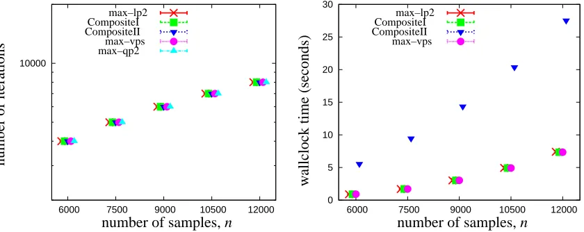
Experiment 2 This experiment compares actual computational requirements for the main loop of various decomposition algorithms applied to the Cyber–Security data. With density level ρ= 1, accuracyε=10−6, parameter values(λ∗,σ∗) = (10−7,10−1) and(λ¯,σ¯) = (.05, .05), and five
different problem sizes n1:n−1 = 2000:4000, 2500:5000, 3000:6000, 3500:7000, and 4000:8000 we employed the decomposition algorithm with Stopping Rule 2 and pair selection methods max– lp2, Composite–I, Composite–II, max–vps and max–qp2. For each problem size we generated ten different training sets by randomly sampling (without replacement) the original data set. Then we ran the decomposition algorithm on each training set and recorded the number of iterations and the wallclock time of the main loop. The minimum, maximum and average values of these quantities for parameter values(λ∗,σ∗) = (10−7,10−1) are shown in Figure 3 4. There is much to discern from the plot on the left. It is easy to verify that for all pair selection methods the numbers of iterations are several orders of magnitude smaller than the worst case bound given in Example 2. On average the convergence rate of the max–lp2 method is much worse than the other methods. This may be partly due to the fact that this method uses only first order information to determine its pair.
However, this is also true of the max–vps method whose convergence rate is much faster. Indeed, it is curious that the max–lp2 method, which chooses a stepwise direction based on a combination of steepness and room to move, has a worse convergence rate than the max–vps method, which chooses a stepwise direction based on steepness alone. By slightly modifying the max–lp2 method to obtain the Composite–I method a much faster convergence rate is observed. The Composite–I
100 1000 10000 100000 12000 10500 9000 7500 6000 max–lp2 CompositeI CompositeII max–qp2max–vps n u mb er o f ite ra tio n s
number of samples, n
0 1 2 3 4 5 12000 10500 9000 7500 6000 max–vps max–lp2 CompositeI CompositeII w allc lo ck time (s ec o n d s)
number of samples, n
Figure 3: Main loop computation for Cyber–Security data with(λ∗,σ∗) = (10−7,10−1).
10000 12000 10500 9000 7500 6000 max–lp2 CompositeI CompositeII max–qp2max–vps n u mb er o f ite ra tio n s
number of samples, n
0 5 10 15 20 25 30 12000 10500 9000 7500 6000 max–vps max–lp2 CompositeI CompositeII w allc lo ck time (s ec o n d s)
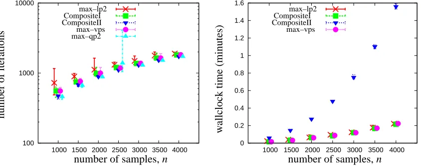
number of samples, n
Figure 4: Main loop computation for Cyber–Security data with(¯λ,σ¯) = (.05, .05). The number of iterations in the left plot is identical for all five methods for all values of n. The wallclock time in the right plot is indistinguishable for the Composite–I, max–vps and max–lp2 methods.