Clustering Hidden Markov Models with Variational HEM

Clustering Hidden Markov Models with Variational HEM

Emanuele Coviello ecoviell@ucsd.edu

Department of Electrical and Computer Engineering University of California, San Diego

La Jolla, CA 92093, USA

Antoni B. Chan abchan@cityu.edu.hk

Department of Computer Science City University of Hong Kong Kowloon Tong, Hong Kong

Gert R.G. Lanckriet gert@ece.ucsd.edu

Department of Electrical and Computer Engineering University of California, San Diego

La Jolla, CA 92093, USA

Editor:Tony Jebara

Abstract

The hidden Markov model (HMM) is a widely-used generative model that copes with sequential data, assuming that each observation is conditioned on the state of a hidden Markov chain. In this paper, we derive a novel algorithm to cluster HMMs based on the hierarchical EM (HEM) algorithm. The proposed algorithm i) clusters a given collection of HMMs into groups of HMMs that are similar, in terms of the distributions they repre-sent, and ii) characterizes each group by a “cluster center”, that is, a novel HMM that is representative for the group, in a manner that is consistent with the underlying generative model of the HMM. To cope with intractable inference in the E-step, the HEM algorithm is formulated as a variational optimization problem, and efficiently solved for the HMM case by leveraging an appropriate variational approximation. The benefits of the proposed algorithm, which we call variational HEM (VHEM), are demonstrated on several tasks involving time-series data, such as hierarchical clustering of motion capture sequences, and automatic annotation and retrieval of music and of online hand-writing data, showing im-provements over current methods. In particular, our variational HEM algorithm effectively leverages large amounts of data when learning annotation models by using an efficient hi-erarchical estimation procedure, which reduces learning times and memory requirements, while improving model robustness through better regularization.

Keywords: Hierarchical EM algorithm, clustering, hidden Markov model, hidden Markov mixture model, variational approximation, time-series classification

1. Introduction

conditioned on the current state. HMMs have been successfully applied to a variety of fields, including speech recognition (Rabiner and Juang, 1993), music analysis (Qi et al., 2007) and identification (Batlle et al., 2002), online hand-writing recognition (Nag et al., 1986), analysis of biological sequences (Krogh et al., 1994), and clustering of time series data (Jebara et al., 2007; Smyth, 1997; Alon et al., 2003).

This paper is about clustering HMMs. More precisely, we are interested in an algorithm that, given a collection of HMMs, partitions them into K clusters of “similar” HMMs, while also learning a representative HMM “cluster center” that concisely and appropriately represents each cluster. This is similar to standard k-means clustering, except that the data points are HMMs now instead of vectors in Rd.

Various applications motivate the design of HMM clustering algorithms, ranging from hi-erarchical clustering of sequential data (e.g., speech or motion sequences modeled by HMMs as by Jebara et al. 2007), to hierarchical indexing for fast retrieval, to reducing the com-putational complexity of estimating mixtures of HMMs from large data sets (e.g., semantic annotation models for music and video)—by clustering HMMs, efficiently estimated from many small subsets of the data, into a more compact mixture model of all data. However, there has been little work on HMM clustering and, therefore, its applications.

The HEM algorithm is a generalization of the EM algorithm—the EM algorithm can be considered as a special case of HEM for a mixture of delta functions as input. The main difference between HEM and EM is in the E-step. While the EM algorithm computes the sufficient statistics given the observed data, the HEM algorithm calculates the expected sufficient statistics averaged over all possible observations generated by the input probability models. Historically, the first HEM algorithm was designed to clusterGaussian probability distributions (Vasconcelos and Lippman, 1998). This algorithm starts from a Gaussian mixture model (GMM) withK(b) components and reduces it to another GMM with fewer components, where each of the mixture components of the reduced GMM represents, that is, clusters, a group of the original Gaussian mixture components. More recently, Chan et al. (2010b) derived an HEM algorithm to cluster dynamic texture (DT) models (i.e., linear dynamical systems, LDSs) through their probability distributions. HEM has been applied successfully to construct GMM hierarchies for efficient image indexing (Vasconcelos, 2001), to cluster video represented by DTs (Chan et al., 2010a), and to estimate GMMs or DT mixtures (DTMs, that is, LDS mixtures) from large data sets for semantic annotation of images (Carneiro et al., 2007), video (Chan et al., 2010a) and music (Turnbull et al., 2008; Coviello et al., 2011). Note that HMMs cannot be clustered by using the original HEM by Vasconcelos and Lippman (1998). Specifically, the original formulation of HEM was designed for clustering data points represented by individual Gaussian models. When clustering HMMs, we are interested in assigning every HMM as a whole to a cluster, and do not want to treat their individual Gaussian states independently. Even with GMMs (as opposed to single Gaussians) this is not possible in closed form, since it would need the expected log likelihood of a mixture.

To extend the HEM framework from clustering Gaussians to clustering HMMs, addi-tional marginalization over the hidden-state processes is required, as with DTs. However, while Gaussians and DTs allow tractable inference in the E-step of HEM, this is no longer the case for HMMs. Therefore, in this work, we derive a variational formulation of the HEM algorithm (VHEM), and then leverage a variationalapproximation derived by Hershey et al. (2007) (which has not been used in a learning context so far) to make the inference in the E-step tractable. The resulting algorithm not only clusters HMMs, but also learns novel HMMs that are representative centers of each cluster. The resulting VHEM algorithm can be generalized to handle other classes of graphical models, for which exact computation of the E-step in the standard HEM would be intractable, by leveraging similar variational approximations—for example, any mixtures of continuous exponential family distributions (e.g., Gaussian) the more general case of HMMs with emission probabilities that are (mix-tures of) continuous exponential family distributions.

intermediate models using the VHEM algorithm. Because VHEM is based on maximum-likelihood principles, it drives model estimation towards similar optimal parameter values as performing maximum-likelihood estimation on the full data set. In addition, by averaging over all possible observations compatible with the input models in the E-step, VHEM pro-vides an implicit form of regularization that prevents over-fitting and improves robustness of the learned models, compared to a direct application of the EM algorithm on the full data set. Note that, in contrast to Jebara et al. (2007), VHEM does not construct a kernel embedding, and is therefore expected to be more efficient, especially for large K(b).

In summary, the contributions of this paper are three-fold: i) we derive a variational for-mulation of the HEM algorithm for clustering HMMs, which generates novel HMM centers representative of each cluster; ii) we evaluate VHEM on a variety of clustering, annota-tion, and retrieval problems involving time-series data, showing improvement over current clustering methods; iii) we demonstrate in experiments that VHEM can effectively learn HMMs from large sets of data, more efficiently than standard EM, while improving model robustness through better regularization. With respect to our previous work, the VHEM algorithm for HMMs was originally proposed by Coviello et al. (2012a)

The remainder of the paper is organized as follows. We review the hidden Markov model (HMM) and the hidden Markov mixture model (H3M) in Section 2. We present the derivation of the VHEM-H3M algorithm in Section 3, followed by a discussion in Section 4.boldsymbol Finally, we present experimental results in Sections 5 and 6.

2. The Hidden Markov (Mixture) Model

A hidden Markov model (HMM)Massumes a sequence ofτ observationsy={y1, . . . , yτ} is generated by a double embedded stochastic process, where each observation (or emission)

ytat timetdepends on the state of a discrete hidden variablext, and the sequence of hidden statesx={x1, . . . , xτ}evolves as a first-order Markov chain. The hidden variables can take one of S values, {1, . . . , S}, and the evolution of the hidden process is encoded in a state transition matrix A = [aβ,β0]_β,β0_=1,...,S, where each entry, a_β,β0 = p(x_t+1 =β0|x_t =β,M),

is the probability of transitioning from stateβ to stateβ0, and an initial state distribution

π= [π1, . . . , πS], whereπβ =p(x1 =β|M).

Each state β generates observations according to an emission probability density func-tion,p(yt|xt=β,M). Here, we assume the emission density istime-invariant, and modeled as a Gaussian mixture model (GMM) withM components:

p(y|x=β,M) = M

X

m=1

cβ,mp(y|ζ =m, x=β,M), (1)

where ζ ∼ multinomial(cβ,1, . . . , cβ,M) is the hidden assignment variable that selects the mixture component, with cβ,m as the mixture weight of the mth component, and each component is a multivariate Gaussian distribution,

p(y|ζ=m, x=β,M) =N(y;µβ,m,Σβ,m),

with mean µβ,mand covariance matrix Σβ,m. The HMM is specified by the parameters

which can be efficiently learned from an observation sequence y with the Baum-Welch algorithm (Rabiner and Juang, 1993), which is based on maximum likelihood estimation.

The probability distribution of a state sequence x generated by an HMMMis

p(x|M) =p(x1|M) τ

Y

t=2

p(xt|xt−1,M) =πx1 τ

Y

t=2

axt−1,xt,

while the joint likelihood of an observation sequence yand a state sequence xis

p(y,x|M) =p(y|x,M)p(x|M) =p(x1|M) τ

Y

t=2

p(xt|xt−1,M) τ

Y

t=1

p(yt|xt,M).

Finally, the observation likelihood ofy is obtained by marginalizing out the state sequence from the joint likelihood,

p(y|M) =X

x

p(y,x|M) =X

x

p(y|x,M)p(x|M), (2)

where the summation is over all state sequences of lengthτ, and can be performed efficiently using theforward algorithm (Rabiner and Juang, 1993).

A hidden Markov mixture model (H3M) (Smyth, 1997) models a set of observation se-quences as samples from a group ofK hidden Markov models, each associated to a specific sub-behavior. For a given sequence, an assignment variable z ∼multinomial(ω1,· · · , ωK) selects the parameters of one of the K HMMs, where thekth HMM is selected with prob-ability ωk. Each mixture component is parametrized by

Mz ={πz, Az,{{czβ,m, µβ,mz ,Σzβ,m}Mm=1}Sβ=1},

and the H3M is parametrized byM={ωz,Mz}Kz=1, which can be estimated from a collec-tion of observacollec-tion sequences using the EM algorithm (Smyth, 1997; Alon et al., 2003).

To reduce clutter, here we assume that all the HMMs have the same numberSof hidden states and that all emission probabilities haveM mixture components. Our derivation could be easily extended to the more general case though.

3. Clustering Hidden Markov Models

Algorithms for clustering HMMs can serve a wide range of applications, from hierarchical clustering of sequential data (e.g., speech or motion sequences modeled by HMMs (Jebara et al., 2007)), to hierarchical indexing for fast retrieval, to reducing the computational complexity of estimating mixtures of HMMs from large weakly-annotated data sets—by clustering HMMs, efficiently estimated from many small subsets of the data, into a more compact mixture model of all data.

One method for estimating the reduced mixture model is to generate samples from the input mixture, and then perform maximum likelihood estimation, that is, maximize the log-likelihood of these samples. However, to avoid explicitly generating these samples, we instead maximize the expectation of the log-likelihood with respect to the input mixture model, thus averaging over all possible samples from the input mixture model. In this way, the dependency on the samples is replaced by a marginalization with respect to the input mixture model. While such marginalization is tractable for Gaussians and DTs, this is no longer the case for HMMs. Therefore, in this work, we i) derive a variational formulation of the HEM algorithm (VHEM), and ii) specialize it to the HMM case by leveraging a variational approximation proposed by Hershey et al. (2007). Note that the work of Hershey et al. (2007) was proposed as an alternative to MCMC sampling for the computation of the KL divergence between two HMMs, and has not been used in a learning context so far.

We present the problem formulation in Section 3.1, and derive the algorithm in Sections 3.2, 3.3 and 3.4.

3.1 Formulation

LetM(b) _{be a base hidden Markov mixture model with K}(b) _{components. The goal of the} VHEM algorithm is to find a reduced hidden Markov mixture modelM(r)_withK(r) _{< K}(b) (i.e., fewer) components that represents M(b) _{well. The likelihood of a random sequence} y∼ M(b) _{is given by}

p(y|M(b)_{) =} K(b)

X

i=1

ω_i(b)p(y|z(b)=i,M(b)_{), (3)}

where z(b) ∼ multinomial(ω₁(b),· · ·ω(b)

K(b)) is the hidden variable that indexes the mixture

components. p(y|z=i,M(b)_{) is the likelihood ofy under theith mixture component, as in} (2), and ω_i(b) is the mixture weight for the ith component. Likewise, the likelihood of the random sequence y∼ M(r) _is

p(y|M(r)) = K(r)

X

j=1

ω_j(r)p(y|z(r)=j,M(r)), (4)

where z(r) ∼ multinomial(ω₁(r),· · · , ω_K(r)(r)) is the hidden variable for indexing components

inM(r)_.

At a high level, the VHEM-H3M algorithm estimates the reduced H3M modelM(r) _in (4) fromvirtual sequences distributed according to the base H3M modelM(b)_{in (3). From} this estimation procedure, the VHEM algorithm provides:

variables base model (b) reduced model (r)

index for HMM components i j

number of HMM components K(b) K(r)

HMM states β ρ

number of HMM states S S

HMM state sequence β={β1,· · ·, βτ} ρ={ρ1,· · ·, ρτ}

index for component of GMM m `

number of Gaussian components M M

models

H3M M(b) _M(r)

HMM component (of H3M) M(b)_i M(r)_j

GMM emission M(b)_i,β M(r)_j,ρ

Gaussian component (of GMM) M(b)_i,β,m M(r)_j,ρ,`

parameters

H3M component weight ω_i(b) ω_j(r)

HMM initial state π(b),i _π(r),j

HMM state transition matrix A(b),i _A(r),j

GMM emission {c(b),i_β,m, µ(b),i_β,m,Σ(b),i_β,m}M

m=1 {c

(r),j ρ,` , µ

(r),j ρ,` ,Σ

(r),j ρ,` }

M `=1

probability distributions notation short-hand

HMM state sequence (b) p(x=β|z(b)_=i,M(b)_{) p(β|M}(b) i ) =π

(b),i

β

HMM state sequence (r) p(x=ρ|z(r)_=j,M(r)_{) p(ρ|M}(r)

j ) =π

(r),j

ρ

HMM observation likelihood (r) p(y|z(r)=j,M(r)_{) p(y|M}(r) j )

GMM emission likelihood (r) p(yt|xt=ρ,M(r)_j ) p(yt|M(r)_j,ρ)

Gaussian component likelihood (r) p(yt|ζt=`, xt=ρ,M(r)<sub>j</sub> ) p(yt|M(r)<sub>j,ρ,`</sub>)

expectations

HMM observation sequence (b) E_y|z(b)_=i,M(b)[·] E

M(_ib)[·]

GMM emission (b) E_y

t|xt=β,M(ib)

[·] E_M(b) i,β

[·]

Gaussian component (b) E_y

t|ζt=m,xt=β,M(ib)

[·] E_M(b) i,β,m

[·]

expected log-likelihood lower bound variational distribution

E_M(b) i

[logp(Yi|M(r)_{)] L}i

H3M qi(zi=j) =zij

E

M(ib)

[logp(y|M(r)_j )] L_{HM M}i,j qi,j(ρ|β) =φi,j_ρ|β

=φi,j1 (ρ1|β1) Qτ

t=2φ i,j

t (ρt|ρt−1, βt)

E

M(_i,βb)[logp(y|M

(r)

j,ρ)] L

(i,β),(j,ρ)

GM M q

i,j

β,ρ(ζ=`|m) =η (i,β),(j,ρ) `|m

Table 1: Notation used in the derivation of the VHEM-H3M algorithm.

2. novel cluster centers represented by the individual mixture components of the reduced model in (4), that is,p(y|z(r)=j,M(r)_{) forj = 1, . . . , K}(r)_.

3.1.1 Notation

We will always useiandjto index the components of the base modelM(b) _{and the reduced} modelM(r)_{, respectively. To reduce clutter, we will also use the short-hand notationM}(b) i andM(_jr)to denote theith component ofM(b)_{and thejth component ofM}(r)_{, respectively.} Hidden states of the HMMs are denoted with β for the base model M(_ib), and with ρ for the reduced model M(_jr).

The GMM emission models for each hidden state are denoted asM(_i,βb)andM(_j,ρr). We will always usemand`for indexing the individual Gaussian components of the GMM emissions of the base and reduced models, respectively. The individual Gaussian components are denoted as M(<sub>i,β,m</sub>b) for the base model, and M(<sub>j,ρ,`</sub>r) for the reduced model. Finally, we denote the parameters of ith HMM component of the base mixture model as M(_ib) = {π(b),i_{, A}(b),i_,{{c(b),i

β,m, µ (b),i β,m,Σ

(b),i

β,m}Mm=1}Sβ=1}, and for the jth HMM in the reduced mixture asM(_jr)={π(r),j, A(r),j,{{c(_{ρ,`</sub>r),j, µ<sub>ρ,`}(r),j,Σ(_ρ,`r),j}M

`=1}Sρ=1}.

When appearing in a probability distribution, the short-hand model notation (e.g., M(_ib)) always implies conditioning on the model being active. For example, we will use

p(y|M(_ib)) as short-hand for p(y|z(b) =i,M(b)_{), or p(y}

t|M(_i,βb)) as short-hand for p(yt|xt = β, z(b) =i,M(b)_{). Furthermore, we will use π}(b),i

β as short-hand for the probability of the

state sequence β according to the base HMM component M(_ib), that is, p(β|M(_ib)), and likewiseM(_ρr),j for the reduced HMM component.

Expectations will also use the short-hand model notation to imply conditioning on the model. In addition, expectations are assumed to be taken with respect to the output variable (y or yt), unless otherwise specified. For example, we will use E_M(b)

i

[·] as short-hand for

E_y|z(b)_=i,M(b)[·].

Table 1 summarizes the notation used in the derivation, including the variable names, model parameters, and short-hand notations for probability distributions and expectations. The bottom of Table 1 also summarizes the variational lower bound and variational distri-butions, which will be introduced subsequently.

3.2 Variational HEM Algorithm

To learn the reduced model in (4), we consider a set of N virtual samples, distributed according to the base model M(b) _{in (3), such that N}

i = N ωi(b) samples are drawn from the ith component. We denote the set of Ni virtual samples for the ith component as Yi = {y(i,m)}mNi=1, where y(i,m) ∼ M

(b)

i , and the entire set of N samples as Y ={Yi}K (b) i=1 . Note that, in this formulation, we are not considering virtual samples {x(i,m)_,y(i,m)_{} for} each base component, according to its joint distributionp(x,y|M(_ib)). The reason is that the hidden-state space of each base mixture componentM(_ib)may have a different representation (e.g., the numbering of the hidden states may be permuted between the components). This mismatch will cause problems when the parameters of M(_jr) are computed from virtual samples of the hidden states of{M(_ib)}K(b)

i=1 . Instead, we treatXi={x(i,m)} Ni

information, and estimate them in the E-step. The log-likelihood of the virtual samples is

logp(Y|M(r)) = K(b)

X

i=1

logp(Yi|M(r)), (5)

where, in order to obtain a consistent clustering, we assume the entirety of samples Yi is assigned to the same component of the reduced model (Vasconcelos and Lippman, 1998).

The original formulation of HEM (Vasconcelos and Lippman, 1998) maximizes (5) with respect to M(r)_{, and uses the law of large numbers to turn the virtual samples Y}

i into an expectation over the base model components M(_ib). In this paper, we will start with a different objective function to derive the VHEM algorithm. To estimateM(r)_{, we will} max-imize the average log-likelihood of all possible virtual samples, weighted by their likelihood of being generated byM(_ib), that is, theexpected log-likelihood of the virtual samples,

J(M(r)_{) = E} M(b)

h

logp(Y|M(r)₎i₌ K(b)

X

i=1 E_M(b)

i h

logp(Yi|M(r))

i

, (6)

where the expectation is over the base model componentsM(_ib). Maximizing (6) will even-tually lead to the same estimate as maximizing (5), but allows us to strictly preserve the variational lower bound, which would otherwise be ruined when applying the law of large numbers to (5).

A general approach to deal with maximum likelihood estimation in the presence of hidden variables (which is the case for H3Ms) is the EM algorithm (Dempster et al., 1977). In the traditional formulation the EM algorithm is presented as an alternation between an expectation step (E-step) and a maximization step (M-step). In this work, we take a variational perspective (Neal and Hinton, 1998; Wainwright and Jordan, 2008; Csisz´ar and Tusn´ady, 1984), which views each step as a maximization step. The variational E-step first obtains a family of lower bounds to the (expected) log-likelihood (i.e., to Equation 6), indexed by variational parameters, and then optimizes over the variational parameters to find the tightest bound. The corresponding M-step then maximizes the lower bound (with the variational parameters fixed) with respect to the model parameters. One advantage of the variational formulation is that it readily allows for useful extensions to the EM algorithm, such as replacing a difficult inference in the E-step with a variational approximation. In practice, this is achieved by restricting the maximization in the variational E-step to a smaller domain for which the lower bound is tractable.

The EM algorithm with variational E-step is guaranteed to converge (Gunawardana and Byrne, 2005). Despite the approximation prevents convergence to local maxima of the data log-likelihood (Gunawardana and Byrne, 2005), the algorithm still performs well empirically, as shown in Section 5 and Section 6.

3.2.1 Lower Bound to an Expected Log-likelihood

standard tool in machine learning (Jordan et al., 1999; Jaakkola, 2000), which we briefly review next. In all generality, let {O, H} be the observation and hidden variables of a probabilistic model, respectively, where p(H) is the distribution of the hidden variables,

p(O|H) is the conditional likelihood of the observations, and p(O) = P

Hp(O|H)p(H) is the observation likelihood. We can define a variational lower bound to the observation log-likelihood (Jordan et al., 1999; Jaakkola, 2000):

logp(O)≥logp(O)−D(q(H)||p(H|O)) =X

H

q(H) logp(H)p(O|H)

q(H) ,

where p(H|O) is the posterior distribution of H given observation O, and D(pkq) =

R

p(y) logp_q(₍y_y))dy is the Kullback-Leibler (KL) divergence between two distributions, p and

q. We introduce a variational distribution q(H), which approximates the posterior dis-tribution, where P

Hq(H) = 1 and q(H) ≥ 0. When the variational distribution equals the true posterior, q(H) =P(H|O), then the KL divergence is zero, and hence the lower-bound reaches logp(O). When the true posterior cannot be computed, then typically q is restricted to some set of approximate posterior distributions Q that are tractable, and the best lower-bound is obtained by maximizing over q∈ Q,

logp(O)≥max q∈Q

X

H

q(H) logp(H)p(O|H)

q(H) . (7)

From the standard lower bound in (7), we can now derive a lower bound to an expected log-likelihood expression. Let Eb[·] be the expectation with respect to O with some dis-tribution pb(O). Since pb(O) is non-negative, taking the expectation on both sides of (7) yields,

Eb[logp(O)]≥Eb

"

max q∈Q

X

H

q(H) logp(H)p(O|H)

q(H)

#

(8)

≥max q∈Q Eb

"

X

H

q(H) logp(H)p(O|H)

q(H)

#

(9)

= max q∈Q

X

H q(H)

logp(H)

q(H) + Eb[logp(O|H)]

, (10)

where (9) follows from Jensen’s inequality (i.e., f(E[x])≤ E[f(x)] when f is convex), and the convexity of the max function. Hence, (10) is a variational lower bound on the expected log-likelihood, which depends on the family of variational distributionsQ.

In (8) we are computing the best lower-bound (7) to logp(O)individually for each value of the observation variableO, which in general corresponds to different optimal q∗∈ Qfor different values of O. Note that the expectation in (8) is not analytically tractable when

3.2.2 Variational Lower Bound

We now derive a lower bound to the expected log-likelihood cost function in (6). The derivation will proceed by successively applying the lower bound from (10) to each expected log-likelihood term that arises. This will result in a set of nested lower bounds.

A variational lower bound to the expected log-likelihood of the virtual samples in (6) is obtained by lower bounding each of the expectation terms E_M(b)

i

in the sum,

J(M(r)) = K(b)

X

i=1 E_M(b)

i h

logp(Yi|M(r))

i

≥ K(b)

X

i=1

Li_H3M, (11)

where we define three nested lower bounds, corresponding to different model elements (the H3M, the component HMMs, and the emission GMMs):

E_M(b)

i

[logp(Yi|M(r))]≥ LiH3M, (12) E_M(b)

i

[logp(y|M(_jr))]≥ Li,j_{HM M}, (13) E_M(b)

i,β

[logp(y|M(_j,ρr))]≥ L(_{GM M}i,β),(j,ρ). (14) In (12), the first lower bound, Li

H3M, is on the expected log-likelihood of an H3M M(r) with respect to an HMM M(_ib). Because p(Yi|M(r)) is the likelihood under a mixture of HMMs, as in (4), where the observation variable is Yi and the hidden variable is zi (the assignment of Yi to a component of M(r)), its expectation cannot be calculated directly. Hence, we introduce the variational distributionqi(zi) and apply (10) to (12), yielding the lower bound (see Appendix A),

Li_H3M = max qi

X

j

qi(zi=j)

(

logp(zi =j|M (r)₎

qi(zi =j)

+NiLi,j_{HM M}

)

. (15)

The lower bound in (15) depends on the second lower bound (Eq. 13), Li,j_{HM M}, which is on the expected log-likelihood of an HMMM(_jr), averaged over observation sequences from a different HMM M(_ib). Although the data log-likelihood logp(y|M(_jr)) can be computed exactly using the forward algorithm (Rabiner and Juang, 1993), calculating its expectation is not analytically tractable since an observation sequenceyfrom a HMMM(_jr)is essentially an observation from a mixture model.1

To calculate the lower bound Li,j_{HM M} in (13), we first rewrite the expectation E_M(b)

i

in

(13) to explicitly marginalize over the state sequenceβofM(_ib), and then apply (10) where the hidden variable is the state sequence ρof M(_jr), yielding (see Appendix A)

Li,j_{HM M} =X

β

π_β(b),imax qi,j

X

ρ

qi,j(ρ|β)

(

logp(ρ|M (r) j ) qi,j_(ρ|β) +

X

t

L(i,βt),(j,ρt)

GM M

)

, (16)

where we introduce a variational distribution qi,j(ρ|β) on the state sequence ρ, which depends on a particular sequenceβ fromM(_ib). As before, (16) depends on another nested lower bound,L(_{GM M}i,β),(j,ρ) in (14), which is on the expected log-likelihood of a GMM emission density M(_j,ρr) with respect to another GMM M(_i,βb). This lower bound does not depend on time, as we have assumed that the emission densities are time-invariant.

Finally, we obtain the lower bound L(_{GM M}i,β),(j,ρ) for (14), by explicitly marginalizing over the GMM hidden assignment variable in M(_i,βb) and then applying (10) to the expectation of the GMM emission distributionp(y|M(_j,ρr)), yielding (see Appendix A),

L(_{GM M}i,β),(j,ρ) = M

X

m=1

c(_β,mb),imax qi,j_β,ρ

M

X

ζ=1

qi,j_β,ρ(ζ|m)

(

logp(ζ|M (r) j,ρ)

q_β,ρi,j(ζ|m) + EM(i,β,mb)

[logp(y|M(_j,ρ,ζr) )]

)

, (17)

where we introduce the variational distributionq_β,ρi,j(ζ|m), which is conditioned on the obser-vationyarising from themth component inM(_i,βb). In (17), the term E_M(b)

i,β,m

[logp(y|M(_{j,ρ,`</sub>r) )] is the expected log-likelihood of the Gaussian distributionM(<sub>j,ρ,`}r) with respect to the Gaus-sian M(_i,β,mb) , which has a closed-form solution (see Section 3.3.1).

In summary, we have derived a variational lower bound to the expected log-likelihood of the virtual samples, which is given by (11). This lower bound is composed of three nested lower bounds in (15), (16), and (17), corresponding to different model elements (the H3M, the component HMMs, and the emission GMMs), where qi(zi), qi,j(ρ|β), and q_β,ρi,j(ζ|m) are the corresponding variational distributions. Finally, the variational HEM algorithm for HMMs consists of two alternating steps:

• (variational E-step) given M(r)_{, calculate the variational distributions}

q_β,ρi,j(ζ|m), qi,j(ρ|β), and qi(zi) for the lower bounds in (17), (16), and (15); • (M-step) update the model parameters viaM(r)∗ _{= argmax}

M(r)

PK(b)

i=1 LiH3M. In the following subsections, we derive the E- and M-steps of the algorithm. The entire procedure is summarized in Algorithm 1.

3.3 Variational E-Step

The variational E-step consists of finding the variational distributions that maximize the lower bounds in (17), (16), and (15). In particular, given the nesting of the lower bounds, we proceed by first maximizing the GMM lower bound L(_{GM M}i,β),(j,ρ) for each pair of emission GMMs in the base and reduced models. Next, the HMM lower boundLi,j_{HM M} is maximized for each pair of HMMs in the base and reduced models, followed by maximizing the H3M lower bound Li

H3M for each base HMM. Finally, a set of summary statistics are calculated, which will be used in the M-step.

3.3.1 Variational Distributions

Algorithm 1 VHEM algorithm for H3Ms

1: Input: base H3MM(b)_={ω(b) i ,M

(b) i }K

(b)

i=1 , number of virtual samples N.

2: Initialize reduced H3MM(r)_={ω(r) j ,M

(r) j }K

(r) j=1.

3: repeat

4: {Variational E-step}

5: Compute optimal variational distributions and variational lower bounds:

6: for each pair of HMMsM(_is) and M(_jr)

7: for eachpair of emission GMMs for state β ofM_i(s) and ρ ofM(_jr):

8: Compute optimal variational distributions ˆη(_`i,β_|m),(j,ρ) as in (18)

9: Compute optimal lower boundL(_{GM M}i,β),(j,ρ) to expected log-likelihood as in (22)

10: Compute optimal variational distributions for HMMs as in Appendin B ˆ

φi,j₁ (ρ1|β1), φˆi,jt (ρt|ρt−1, βt) for t=τ, . . . ,2

11: Compute optimal lower boundLi,j_{HM M} to expected log-likelihood as in (21)

12: Compute optimal assignment probabilities:

ˆ

zij =

ω_j(r)exp(N ω_i(b)Li,j_{HM M})

P

j0ω

(r)

j0 exp(N ω

(b) i L

i,j0

HM M)

13: Compute aggregate summary statistics for each pair of HMMsM(_is) and M(_jr) as in Section 3.3.3:

ˆ

ν₁i,j(ρ) = S

X

β=1

ν₁i,j(ρ, β), νˆi,j(ρ, β) = τ

X

t=1

ν_ti,j(ρ, β), ξˆi,j(ρ, ρ0) = τ

X

t=2 S

X

β=1

ξi,j_t (ρ, ρ0, β)

14: {M-step}

15: For each component M(_jr), recompute parameters using (24)-(28).

16: untilconvergence

17: Output: reduced H3M {ω_j(r),M(_ja)}K(r) j=1.

GMM: For the GMM lower boundL(_{GM M}i,β),(j,ρ), we assume each variational distribution has the form (Hershey et al., 2007)

q_β,ρi,j(ζ =l|m) =η_`(_|i,β_m),(j,ρ),

wherePM

`=1η

(i,β),(j,ρ)

`|m = 1, andη

(i,β),(j,ρ)

`|m ≥0,∀`. Intuitively,η

(i,β),(j,ρ) _{is the responsibility} matrix between each pair of Gaussian components in the GMMs M(_i,βb) and M(_j,ρr), where

parameters yields (see Appendix B)

ˆ

η_`(_|i,β_m),(j,ρ)=

c(_ρ,`r),jexp

E_M(b)

i,β,m

[logp(y|M(_j,ρ,`r) )]

P

`0c(<sub>ρ,`</sub>r)0,jexp

E_M(b)

i,β,m

[logp(y|M(_j,ρ,`r) 0)]

, (18)

where the expected log-likelihood of a Gaussian M(_j,ρ,`r) with respect to another Gaussian M(_i,β,mb) is computable in closed-form (Penny and Roberts, 2000),

E_M(b)

i,β,m

[logp(y|M(_j,ρ,`r) )] =−d

2log 2π− 1 2log

Σ

(r),j ρ,`

−

1 2tr

(Σ(_ρ,`r),j)−1Σ(_β,mb),i −1

2(µ (r),j ρ,` −µ

(b),i β,m)

T_(Σ(r),j ρ,` )

−1_(µ(r),j ρ,` −µ

(b),i β,m).

HMM: For the HMM lower bound Li,j_{HM M}, we assume each variational distribution takes the form of a Markov chain,

qi,j(ρ|β) =φi,j(ρ|β) =φi,j₁ (ρ1|β1) τ

Y

t=2

φi,j_t (ρt|ρt−1, βt),

where PS

ρ1=1φ i,j

1 (ρ1|β1) = 1, and PSρt=1φ

i,j

t (ρt|ρt−1, βt) = 1, and all the factors are non-negative. The variational distribution qi,j(ρ|β) represents the probability of the state se-quenceρin HMM M(_jr), when M(_jr) is used to explain theobservationsequence generated by M(_ib) that evolved through state sequenceβ.

Substituting φi,j into (16), the maximization with respect to φi,j_t (ρt|ρt−1, βt) and φi,j₁ (ρ1|β1) is carried out independently for each pair (i, j), and follows (Hershey et al., 2007). This is further detailed in Appendix B. By separating terms and breaking up the summation overβand ρ, the optimal ˆφi,j_t (ρt|ρt−1, βt) and ˆφi,j₁ (ρ1|β1) can be obtained using an efficient recursive iteration (similar to the forward algorithm).

H3M: For the H3M lower bound Li

H3M, we assume variational distributions of the form qi(zi = j) = zij, where PK

(r)

j=1 zij = 1, and zij ≥ 0. Substituting zij into (15), and maximizing variational parameters are obtained as (see Appendix B)

ˆ

zij =

ω(_jr)exp(NiLi,j_{HM M})

P

j0ω

(r)

j0 exp(NiLi,j

0

HM M)

. (19)

Note that in the standard HEM algorithm (Vasconcelos and Lippman, 1998; Chan et al., 2010a), the assignment probabilities zij are based on the expected log-likelihoods of the components, (e.g., E_M(b)

i

3.3.2 Lower Bound

Substituting the optimal variational distributions into (15), (16), and (17) gives the lower bounds,

Li H3M =

X j ˆ zij ( logω (r) j ˆ

zij

+NiLi,jHM M

)

, (20)

Li,j_{HM M} =X

β

π_β(b),iX

ρ

ˆ

φi,j(ρ|β)

(

log π (r),j

ρ

ˆ

φi,j_(ρ|β) +

X

t

L(i,βt),(j,ρt)

GM M

)

, (21)

L(_{GM M}i,β),(j,ρ)= M

X

m=1

c(_β,mb),i M

X

`=1 ˆ

η(_`i,β_|m),(j,ρ)







log c (r),j ρ,`

ˆ

η_`(_|i,β_m),(j,ρ)

+ E_M(b)

i,β,m

[logp(y|M(_j,ρ,`r) )]







. (22)

The lower bound Li,j_{HM M} requires summing over all sequences β and ρ. This summation can be computed efficiently along with ˆφi,j_t (ρt|ρt−1, βt) and ˆφi,j₁ (ρ1|β1) using a recursive algorithm from Hershey et al. (2007). This is described in Appendix B.

3.3.3 Summary Statistics

After calculating the optimal variational distributions, we calculate the following summary statistics, which are necessary for the M-step:

ν₁i,j(ρ1, β1) =π_β(b₁),iφˆ1i,j(ρ1|β1),

ξ_ti,j(ρt−1, ρt, βt) =





S

X

βt−1=1

ν_ti,j₋₁(ρt−1, βt−1)a(_βb_t)₋,i_1,βt



φˆ

i,j

t (ρt|ρt−1, βt), fort= 2, . . . , τ,

ν_ti,j(ρt, βt) = S

X

ρt−1=1

ξ_ti,j(ρt−1, ρt, βt), fort= 2, . . . , τ,

and the aggregate statistics

ˆ

ν₁i,j(ρ) = S

X

β=1

ν₁i,j(ρ, β), (23)

ˆ

νi,j(ρ, β) = τ

X

t=1

ν_ti,j(ρ, β),

ˆ

ξi,j(ρ, ρ0) = τ X t=2 S X β=1

ξi,j_t (ρ, ρ0, β).

The statistic ˆν₁i,j(ρ) is the expected number of times that the HMMM(_jr) starts from state

is the expected number of transitions from state ρ to state ρ0 of the HMM M(_jr), when modeling sequences generated byM(_ib).

3.4 M-Step

In the M-step, the lower bound in (11) is maximized with respect to the parametersM(r)_,

M(r)∗= argmax M(r)

K(b)

X

i=1

Li_H3M.

The derivation of the maximization is presented in Appendix C. Each mixture component of M(r) _{is updated independently according to}

ω_j(r)∗ =

PK(b)

i=1 zˆi,j

K(b) , (24)

π(_ρr),j∗ =

PK(b)

i=1 zˆi,jω (b) i νˆ

i,j 1 (ρ)

PS

ρ0₌₁PK

(b)

i=1 zˆi,jωi(b)νˆ i,j 1 (ρ0))

, a(_ρ,ρr),j0

∗ =

PK(b)

i=1 zˆi,jω (b)

i ξˆi,j(ρ, ρ 0₎

PS

σ=1

PK(b)

i=1 zˆi,jω(ib)ξˆi,j(ρ, σ)

, (25)

c(_ρ,`r),j∗ =

Ωj,ρ

ˆ

η_`(i,β_|m),(j,ρ)

PM

`0₌₁Ω_j,ρ

ˆ

η_`(i,β0_|m),(j,ρ)

, µ

(r),j ρ,`

∗ =

Ωj,ρ

η_`(_|i,β_m),(j,ρ) µ(_β,mb),i

Ωj,ρ

ˆ

η(_`i,β_|m),(j,ρ)

, (26)

Σ(_ρ,`r),j∗ = Ωj,ρ

ˆ

η_`(_|i,β_m),(j,ρ)

h

Σ_β,m(b),i+ (µ(_β,mb),i−µ_{ρ,`</sub>(r),j)(µ(<sub>β,m</sub>b),i−µ(<sub>ρ,`}r),j)T

i

Ωj,ρ

ˆ

η(_`i,β_|m),(j,ρ)

, (27)

where Ωj,ρ(·) is the weighted sum operator over all base models, HMM states, and GMM components (i.e., over all tuples (i, β, m)),

Ωj,ρ(f(i, β, m)) = K(b)

X

i=1 ˆ

zi,jω(_ib) S

X

β=1 ˆ

νi,j(ρ, β) M

X

m=1

c(_β,mb),if(i, β, m). (28)

The termsπ(ρr),j anda_ρ,ρ(r),j0 are elements of the initial state prior and transition matrix,π(r),j

and A(r),j. Note that the covariance matrices of the reduced models in (27) include an additional outer-product term, which acts to regularize the covariances of the base models. This regularization effect derives from the E-step, which averages all possible observations from the base model.

4. Applications and Related Work

4.1 Applications of the VHEM-H3M Algorithm

The proposed VHEM-H3M algorithm clusters HMMsdirectly through the distributions they represent, and learnsnovel HMM cluster centers that compactly represent the structure of each cluster.

An application of the VHEM-H3M algorithm is in hierarchical clustering of HMMs. In particular, the VHEM-H3M algorithm is used recursively on the HMM cluster centers, to produce a bottom-up hierarchy of the input HMMs. Since the cluster centers condense the structure of the clusters they represent, the VHEM-H3M algorithm can implicitly leverage rich information on the underlying structure of the clusters, which is expected to impact positively the quality of the resulting hierarchical clustering.

Another application of VHEM is for efficient estimation of H3Ms from data, by using a hierarchical estimation procedure to break the learning problem into smaller pieces. First, a data set is split into small (non-overlapping) portions and intermediate HMMs are learned for each portion, via standard EM. Then, the final model is estimated from the intermediate models using the VHEM-H3M algorithm. Because VHEM and standard EM are based on similar maximum-likelihood principles, it drives model estimation towards similar optimal parameter values as performing EM estimation directly on the full data set. However, compared to direct EM estimation, VHEM-H3M is more memory- and time-efficient. First, it no longer requires storing in memory the entire data set during parameter estimation. Second, it does not need to evaluate the likelihood of all the samples at each iteration, and converges to effective estimates in shorter times. Note that even if a parallel implementation of EM could effectively handle the high memory requirements, a parallel-VHEM will still require fewer resources than a parallel-EM.

In addition, for the hierarchical procedure, the estimation of the intermediate models can be easily parallelized, since they are learned independently of each other. Finally, hi-erarchical estimation allows for efficient model updating when adding new data. Assuming that the previous intermediate models have been saved, re-estimating the H3M requires learning the intermediate models of only the new data, followed by running VHEM again. Since estimation of the intermediate models is typically as computationally intensive as the VHEM stage, reusing the previous intermediate models will lead to considerable computa-tional savings when re-estimating the H3M.

In hierarchical estimation (EM on each time-series, VHEM on intermediate models), VHEM implicitly averages over all possible observations (virtual variations of each time-series) compatible with the intermediate models. We expect this to regularize estimation, which may result in models that generalize better (compared to estimating models with direct EM). Lastly, the “virtual” samples (i.e., sequences), which VHEM implicitly generates for maximum-likelihood estimation, need not be of the same length as the actual input data for estimating the intermediate models. Making the virtual sequences relatively short will positively impact the run time of each VHEM iteration. This may be achieved without loss of modeling accuracy, as show in Section 6.3.

4.2 Related Work

PPK-SC. In particular, the PPK similarity between two HMMs, M(a) _{and M}(b)_{, is defined as}

k(a, b) =

Z

p(y|M(a))λp(y|M(b))λdy, (29) whereλis a scalar, andτ is the length of “virtual” sequences. The caseλ= 1₂ corresponds to the Bhattacharyya affinity. While this approach indirectly leverages the probability dis-tributions represented by the HMMs (i.e., the PPK affinity is computed from the probability distributions of the HMMs) and has proven successful in grouping HMMs into similar clus-ters (Jebara et al., 2007), it has several limitations. First, the spectral clustering algorithm cannot produce novel HMM cluster centers to represent the clusters, which is suboptimal for several applications of HMM clustering. For example, when implementing hierarchi-cal clustering in the spectral embedding space (e.g., using hierarchihierarchi-cal k-means clustering), clusters are represented by single points in the embedding space. This may fail to capture information on the local structure of the clusters that, when using VHEM-H3M, would be encoded by the novel HMM cluster centers. Hence, we expect VHEM-H3M to produce better hierarchical clustering than the spectral clustering algorithm, especially at higher levels of the hierarchy. This is because, when building a new level, VHEM can leverage more information from the lower levels, as encoded in the HMM cluster centers.

One simple extension of PPK-SC to obtain a HMM cluster center is to select the input HMM that the spectral clustering algorithm maps closest to the spectral clustering center. However, with this method, the HMM cluster centers are limited to be one of the existing input HMMs (i.e., similar to the k-medoids algorithm by Kaufman and Rousseeuw 1987), instead of the HMMs that optimally condense the structure of the clusters. Therefore, we expect the novel HMM cluster centers learned by VHEM-H3M to better represent the clusters. A more involved, “hybrid” solution is to learn the HMM cluster centers with VHEM-H3M after obtaining clusters with PPK-SC—using the VHEM-H3M algorithm to summarize all the HMMs within each PPK-SC cluster into a single HMM. However, we expect our VHEM-H3M algorithm to learn more accurate clustering models, since it jointly learns the clustering and the HMM centers, by optimizing a single objective function (i.e., the lower bound to the expected log-likelihood in Equation 11).

A second drawback of the spectral clustering algorithm is that the construction and the inversion of the similarity matrix between the input HMMs is a costly operation when their number is large2 (e.g., see the experiment on H3M density estimation on the music data in Section 6.1). Therefore, we expect VHEM-H3M to be computationally more efficient than the spectral clustering algorithm since, bydirectlyoperating on the probability distributions of the HMMs, it does not require the construction of an initial embedding or any costly matrix operation on large kernel matrices.

Finally, as Jebara et al. (2004) note, the exact computation of (29) cannot be carried out efficiently, unless λ = 1. For different values of λ,3 Jebara et al. (2004) propose to approximate k(a, b) with an alternative kernel function that can be efficiently computed;

2. The computational complexity of large spectral clustering problems can be alleviated by means of numerical techniques for the solutions of eigenfunction problems such as the Nystr¨om method (Nystr¨om, 1930; Fowlkes et al., 2004), or by sampling only part of the similarity matrix and using a sparse eigen-sonver (Achlioptas et al., 2002).

this alternative kernel function, however, is not guaranteed to be invariant to different but equivalent representations of the hidden state process (Jebara et al., 2004).4 Alternative approximations for the Bhattacharyya setting (i.e., λ= 1₂) have been proposed by Hershey and Olsen (2008).

Note that spectral clustering algorithms (similar to the one by Jebara et al. 2007) can be applied to kernel (similarity) matrices that are based on other affinity scores between HMM distributions than the PPK similarity of Jebara et al. (2004). Examples can be found in earlier work on HMM-based clustering of time-series, such as by Juang and Rabiner (1985), Lyngso et al. (1999), Bahlmann and Burkhardt (2001), Panuccio et al. (2002). In particular, Juang and Rabiner (1985) propose to approximate the (symmetrised) log-likelihood between two HMM distributions by computing the log-likelihood of real samples generated by one model under the other.5 Extensions of the work of Juang and Rabiner (1985) have been proposed by Zhong and Ghosh (2003) and Yin and Yang (2005). In this work we do not pursue a comparison of the various similarity functions, but implement spectral clustering only based on PPK similarity (which Jebara et al. 2007 showed to be superior).

HMMs can also be clustered by sampling a number of time-series from each of the HMMs in the base mixture, and then applying the EM algorithm for H3Ms (Smyth, 1997), to cluster the time-series. Despite its simplicity, this approach would suffer from high memory and time requirements, especially when dealing with a large number of input HMMs. First, all generated samples need to be stored in memory. Second, evaluating the likelihood of the generated samples at each iteration is computationally intensive, and prevents the EM algorithm from converging to effective estimates in acceptable times.6 On the contrary, VHEM-H3M is more efficient in computation and memory usage, as it replaces a costly sampling step (along with the associated likelihood computations at each iteration) with an expectation. An additional problem of EM with sampling is that, with a simple application of the EM algorithm, time-series generated from the same input HMM can be assigned to different clusters of the output H3M. As a consequence, the resulting clustering is not necessary consistent, since in this case the corresponding input HMM may not be clearly assigned to any single cluster. In our experiments, we circumvent this problem by defining appropriate constrains on the assignment variables.

The VHEM algorithm is similar in spirit to Bregman-clustering by Banerjee et al. (2005). Both algorithms base clustering on KL-divergence—the KL divergence and the expected

4. The kernel in (29) is computed by marginalizing out the hidden state variables, that is,

RP

xp(y,x|M

(a) )

λ

P

xp(y,x|M

(b) )

λ

dy. This can be efficiently solved with the junction tree

algorithm only whenλ= 1. Forλ6= 1, Jebara et al. (2004) propose to use an alternative kernel ˜k that applies the power operation to the terms of the sum rather than the entire sum, where the terms are

joint probabilitiesp(y,x). I.e., ˜k(a, b) =R P

x

p(y,x|M(a)₎λP

x

p(y,x|M(b)₎λ_dy. 5. For two HMM distributions,M(a)

andM(b)

, Juang and Rabiner (1985) consider the affinityL(a, b) = 1

2

h

logp(Yb|M(a)) +p(Ya|M(b))

i

, whereYaandYbare sets of observation sequences generated fromM(a)

andM(b)

, respectively.

log-likelihood differ only for an entropy term that does not affect the clustering.7 The main differences are: 1) in our setting, the expected log-likelihood (and KL divergence) is not computable in closed form, and hence VHEM uses an approximation; 2) VHEM-H3M clusters randomprocesses (i.e., time series models), whereas Bregman-clustering (Banerjee et al., 2005) is limited to single random variables. Note that the number of virtual observa-tionsN allows to control thepeakiness of the assignments ˆzi,j. Limiting cases for N → ∞ and N = 1 are similar to Bregman hard and soft cluttering, respectively (Goldberger and Roweis, 2004; Banerjee et al., 2005; Dhillon, 2007).

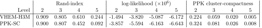
In the next two sections, we validate the points raised in this discussion through exper-imental evaluation using the VHEM-H3M algorithm. In particular, we consider clustering experiments in Section 5, and H3M density estimation for automatic annotation and re-trieval in Section 6. Each application exploits some of the benefits of VHEM. First, we show that VHEM-H3M is more accurate in clustering than PPK-SC, in particular at higher levels of a hierarchical clustering (Section 5.2), and in an experiment with synthetic data (Section 5.3). Similarly, the annotation and retrieval results in Section 6 favor VHEM-H3M over PPK-SC and over standard EM, suggesting that VHEM-H3M is more robust and ef-fective for H3M density estimation. Finally, in all the experiments, the running time of VHEM-H3M compares favorably with the other HMM clustering algorithms; PPK-SC suf-fers long delays when the number of input HMMs is large and the standard EM algorithm is considerably slower. This demonstrates that VHEM-H3M is most efficient for clustering HMMs.

5. Clustering Experiments

In this section, we present an empirical study of the VHEM-H3M algorithm for clustering and hierarchical clustering of HMMs. Clustering HMMs consists in partitioning K1 input HMMs into K2 < K1 groups of similar HMMs. Hierarchical clustering involves organizing the input HMMs in a multi-level hierarchy withhlevels, by applying clustering in a recursive manner. Each level` of the hierarchy has K` groups (with K1 > K2 >· · ·> Kh−1 > Kh), and the first level consists of theK1 input HMMs.

We begin with an experiment on hierarchical clustering, where each of the input HMMs to be clustered is estimated on a sequence of motion capture data (Section 5.2). Then, we present a simulation study on clustering synthetic HMMs (Section 5.3). First, we provide an overview of the different algorithms used in this study.

5.1 Clustering Methods

In the clustering experiments, we will compare our VHEM-H3M algorithm with several other clustering algorithms. The various algorithms are summarized here.

• VHEM-H3M: We clusterK1input HMMs intoK2clusters by using the VHEM-H3M algorithm (on the input HMMs) to learn a H3M with K2 components (as explained

7. We can show that the VHEM algorithm performs clustering based on KL divergence. LettingDi,j

HM M =

Li,i HM M− L

i,j

HM M ≈D(M

(b)

i ||M

(r)

j ) be an approximation to the KL using (21), we can rewrite the E-step

as ˆzij∝ω

(r)

j e

−N ω(_ib)D_{HM M}i,j

. Similarly, the M-step is ˆM(_jr)= arg min

M(_jr)

PK(b) i=1 ω

(b)

in Section 3.1). To build a multi-level hierarchy of HMMs withhlevels, we start from the first level of K1 input HMMs, and recursively use the VHEM-H3M algorithm

h−1 times. Each new level`is formed by clustering theK`−1 HMMs at the previous level into K` < K`−1 groups with the VHEM-H3M algorithm, and using the learned HMMs as cluster centers at the new level. In our experiments, we set the number of virtual samples toN = 104K(`−1), a large value that favors “hard” clustering (where each HMM is univocally assigned to a single cluster), and the length of the virtual sequences toτ = 10.

• PPK-SC: Jebara et al. (2007) cluster HMMs by calculating a PPK similarity ma-trix between all HMMs, and then applying spectral clustering. The work in Jebara et al. (2007) only considered HMMs with single Gaussian emissions, which did not always give satisfactory results in our experiments. Hence, we extended the method of Jebara et al. (2007) by allowing GMM emissions, and derived the PPK similarity for this more general case (Jebara et al., 2004). From preliminary experiments, we found the best performance for PPK with λ = 1₂ (i.e., Bhattacharyya affinity), and when integrating over sequences of length τ = 10. Finally, we also extend Jebara et al. (2007) to construct multi-level hierarchies, by using hierarchical k-means in the spectral clustering embedding.

• SHEM-H3M: This is a version of HEM-H3M that maximizes the likelihood ofactual samples generated from the input HMMs, as in (5), rather than the expectation of virtual samples, as in (6). In particular, from each input HMMM(_ib) we sample a set

Yi of Ni =π(_ib)N observation sequences (for a large value of N). We then estimate the reduced H3M from theN samples Y ={Yi}K

(b)

i=1 , with the EM-H3M algorithm of Smyth (1997), which was modified to use a single assignment variable for each sample setYi, to obtain a consistent clustering.

In many real-life applications, the goal is to cluster a collection of time series, that is, observed sequences. Although the input data is not a collection of HMMs in that case, it can still be clustered with the VHEM-H3M algorithm by first modeling each sequence as an HMM, and then using the HMMs as input for the VHEM-H3M algorithm. With time-series data as input, it is also possible to use clustering approaches that do not model each sequence as a HMM. Hence, in one of the hierarchical motion clustering experiments, we also compare to the following two algorithms, one that clusters time-series data directly (Smyth, 1997), and a second one that clusters the time series after modeling each sequence with a dynamic texture (DT) model (Chan et al., 2010a).

• EM-H3M: The EM algorithm for H3Ms (Smyth, 1997) is applied directly on a col-lection of time series to learn the clustering and HMM cluster centers, thus bypassing the intermediate HMM modeling stage. To obtain a hierarchical clustering (with

level of the hierarchy. This modification preserves the hierarchical clustering property that sequences in a cluster will remain together at the higher levels.

• HEM-DTM: Rather than use HMMs, we consider a clustering model based on linear dynamical systems, that is, dynamic textures (DTs) (Doretto et al., 2003). Hierar-chical clustering is performed using the hierarHierar-chical EM algorithm for DT mixtures (HEM-DTM) (Chan et al., 2010a), in an analogous way to VHEM-H3M. The main difference is that, with HEM-DTM, time-series are modeled as DTs, which have a con-tinuousstate space (a Gauss-Markov model) andunimodalobservation model, whereas VHEM-H3M uses adiscrete state space and multimodalobservations (GMMs).

We will use several metrics to quantitatively compare the results of different clustering algorithms. First, we will calculate the Rand-index (Hubert and Arabie, 1985), which measures the correctness of a proposed clustering against a given ground truth clustering. Intuitively, this index measures how consistent cluster assignments are with the ground truth (i.e., whether pairs of items are correctly or incorrectly assigned to the same cluster, or different clusters). Second, we will consider the log-likelihood, as used by Smyth (1997) to evaluate a clustering. This measures how well the clustering fits the input data. When time series are given as input data, we compute the log-likelihood of a clustering as the sum of the log-likelihoods of each input sequence under the HMM cluster center to which it has been assigned. When the input data consists of HMMs, we will evaluate the log-likelihood of a clustering by using the expected log-likelihood of observations generated from an input HMM under the HMM cluster center to which it is assigned. For PPK-SC, the cluster center is estimated by running the VHEM-H3M algorithm (withK(r)= 1) on the HMMs assigned to the cluster.8 Note that the log-likelihood will be particularly appropriate to compare VHEM-H3M, SHEM-H3M, EM-H3M and HEM-DTM, since they explicitly optimize for it. However, it may be unfair for PPK-SC, since this method optimizes the PPK similarity and not the log-likelihood. As a consequence, we also measure the PPK cluster-compactness, which is more directly related to what PPK-SC optimizes for. The PPK cluster-compactness is the sum (over all clusters) of the average intra-cluster PPK pair-wise similarity. This performance metric favors methods that produce clusters with high intra-cluster similarity. Note that,time seriescan also be clustered with recourse to similarity measures based on dynamic time warping (Oates et al., 1999; Keogh and Pazzani, 2000; Keogh and Ratanama-hatana, 2005) or methods that rely on non-parametric sequence kernels (Leslie et al., 2002; Campbell, 2003; Kuksa et al., 2008; Cortes et al., 2008), which have shown good perfor-mance in practice. In this work we focus on the problem of clusteringhidden Markov models, so we do not pursue an empirical evaluation of these methods.

5.2 Hierarchical Motion Clustering

In this experiment we test the VHEM algorithm on hierarchical motion clustering from motion capture data, that is, time series representing human locomotions and actions. To hierarchically cluster a collection of time series, we first model each time series with an HMM and then cluster the HMMs hierarchically. Since each HMM summarizes the appearance

(a) “Walk” sequence.

(b) “Run” sequence.

Figure 1: Examples of motion capture sequences from the MoCap data set, shown with stick figures.

and dynamics of the particular motion sequence it represents, the structure encoded in the hierarchy of HMMs directly applies to the original motion sequences. Jebara et al. (2007) uses a similar approach to cluster motion sequences, applying PPK-SC to cluster HMMs. However, they did not extend their study to hierarchies with multiple levels.

5.2.1 Data Sets and Setup

We experiment on two motion capture data sets, the MoCap data set (http://mocap.cs.

cmu.edu/) and the Vicon Physical Action data set (Theodoridis and Hu, 2007; Asuncion and

Newman, 2010). For the MoCap data set, we use 56 motion examples spanning 8 different classes (“jump”, “run”, “jog”, “walk 1”, “walk 2”, “basket”, “soccer”, and “sit”). Each example is a sequence of 123-dimensional vectors representing the (x, y, z)-coordinates of 41 body markers tracked spatially through time. Figure 1 illustrates some typical examples. We built a hierarchy of h = 4 levels. The first level (Level 1) was formed by the K1 = 56 HMMs learned from each individual motion example (withS = 4 hidden states, andM = 2 components for each GMM emission). The next three levels contain K2 = 8, K3 = 4 and

K4 = 2 HMMs. We perform the hierarchical clustering with VHH3M, PPK-SC, EM-H3M, SHEM-H3M (N ∈ {560,2800} and τ = 10), and HEM-DTM (state dimension of 7). The experiments were repeated 10 times for each clustering method, using different random initializations of the algorithms.

1 2 L e ve l 4

1 2 3 4

L

e

ve

l

3

1 2 3 4 5 6 7 8

L e ve l 2 1 2 L e ve l 4

1 2 3 4

L

e

ve

l

3

1 2 3 4 5 6 7 8

L

e

ve

l

2

5 10 15 20 25 30 35 40 45 50 55

L

e

ve

l

1

walk 1 jump run jog basket soccer walk 2 sit

VHEM algorithm PPK-SC

so cce r soccer soccer soccer soccer soccer soccer soccer ju mp ju mp jump jump jump jump walk 1 walk 1 walk 1 w a lk 1 walk 1 walk 1 run _run ru n ru n run run

walk 2 walk 2

w a lk 2 w a lk 2 walk 2 walk 2 walk 2 jog jog jog jog jo

g _jog

basket basket basket b a ske t basket basket si t si t sit sit sit sit sit

Figure 2: An example of hierarchical clustering of the MoCap data set, with VHEM-H3M and PPK-SC. Different colors represent different motion classes. Vertical bars represent clusters, with the colors indicating the proportions of the motion classes in a cluster, and the numbers on the x-axes representing the clusters’ indexes. At Level 1 there are 56 clusters, one for each motion sequence. At Levels 2, 3 and 4 there are 8, 4 and 2 HMM clusters, respectively. For VHEM almost all clusters at Level 2 are populated by examples from a single motion class. The error of VHEM in clustering a portion of “soccer” with “basket” is probably because both actions involve a sequence of movement, shot, and pause. Moving up the hierarchy, the VHEM algorithm clusters similar motions classes together, and at Level 4 creates a dichotomy between “sit” and the other (more dynamic) motion classes. PPK-SC also clusters motion sequences well at Level 2, but incorrectly aggregates “sit” and “soccer”, which have quite different dynamics. At Level 4, the clustering obtained by PPK-SC is harder to interpret than that by VHEM.

In similar experiments where we varied the number of levels h of the hierarchy and the number of clusters at each level, we noted similar relative performances of the various clustering algorithms, on both data sets.

5.2.2 Results on the MoCap Data Set

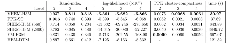
Rand-index log-likelihood (×106_{) PPK cluster-compactness time (s)}

Level 2 3 4 2 3 4 2 3 4

VHEM-H3M 0.937 0.811 0.518 -5.361 -5.682 -5.866 0.0075 0.0068 0.0061 30.97

PPK-SC 0.956 0.740 0.393 -5.399 -5.845 -6.068 0.0082 0.0021 0.0008 37.69

SHEM-H3M (560) 0.714 0.359 0.234 -13.632 -69.746 -275.650 0.0062 0.0034 0.0031 843.89

SHEM-H3M (2800) 0.782 0.685 0.480 -14.645 -30.086 -52.227 0.0050 0.0036 0.0030 3849.72

EM-H3M 0.831 0.430 0.340 -5.713 -202.55 -168.90 0.0099 0.0060 0.0056 667.97

HEM-DTM 0.897 0.661 0.412 -7.125 -8.163 -8.532 - - - 121.32

Table 2: Hierarchical clustering of the MoCap data set using VHEM-H3M, PPK-SC, H3M, EM-H3M and HEM-DTM. The number in brackets after SHEM-H3M represents the number of real samples used. We computed Rand-index, data log-likelihood and cluster compactness at each level of the hierarchy, and reg-istered the time (in seconds) to learn the hierarchical structure. Differences in Rand-index at Levels 2, 3, and 4 are statistically significant based on a paired t-test with confidence 95%.

group similar motions together. We note an error of VHEM in clustering a portion of the “soccer” examples with “basket”. This is probably caused by the fact that both types of actions begin with a stationary phase (e.g., subject focusing on the execution) followed with a forward movement (note that our “basket” examples correspond to forward dribbles). Moving up the hierarchy, the VHEM algorithm clusters similar motion classes together (as indicated by the arrows), for example “walk 1” and “walk 2” are clustered together at Level 2, and at the highest level (Level 4) it creates a dichotomy between “sit” and the rest of the motion classes. This is a desirable behavior as the kinetics of the “sit” sequences (which in the MoCap data set correspond to starting in a standing position, sitting on a stool, and returning to a standing position) are considerably different from the rest. On the right of Figure 2, the same experiment is repeated with PPK-SC. PPK-SC clusters motion sequences properly, but incorrectly aggregates “sit” and “soccer” at Level 2, even though they have quite different dynamics. Furthermore, the highest level (Level 4) of the hierarchical clustering produced by PPK-SC is harder to interpret than that of VHEM.

Comparing to other methods (also in Table 2), EM-H3M generally has lower Rand-index than VHEM-H3M and PPK-SC (consistent with the results from Jebara et al. (2007)). While EM-H3M directly clusters the original motion sequences, both VHEM-H3M and PPK-SC implicitly integrate over all possible virtual variations of the original motion se-quences (according to the intermediate HMM models), which results in more robust cluster-ing procedures. In addition, EM-H3M has considerably longer runncluster-ing times than VHEM-H3M and PPK-SC (i.e., roughly 20 times longer) since it needs to evaluate the likelihood of all training sequences at each iteration, at all levels.

The results in Table 2 favor VHEM-H3M over SHEM-H3M, and empirically validate the variational approximation that VHEM uses for learning. For example, when using

N = 2800 samples, running SHEM-H3M takes over two orders of magnitude more time than VHEM-H3M, but still does not achieve performance competitive with VHEM-H3M. With an efficient closed-form expression for averaging over all possible virtual samples, VHEM approximates the sufficient statistics of a virtually unlimited number of observation sequences, without the need of using real samples. This has an additional regularization effect that improves the robustness of the learned HMM cluster centers. In contrast, SHEM-H3M uses real samples, and requires a large number of them to learn accurate models, which results in significantly longer running times.

In Table 2, we also report hierarchical clustering performance for HEM-DTM. VHEM-H3M consistently outperforms HEM-DTM, both in terms of Rand-index and data log-likelihood.9 Since both VHEM-H3M and HEM-DTM are based on the hierarchical EM algorithm for learning the clustering, this indicates that HMM-based clustering models are more appropriate than DT-based models for the human MoCap data. Note that, while PPK-SC is also HMM-based, it has a lower Rand-index than HEM-DTM at Level 4. This further suggests that PPK-SC does not optimally cluster the HMMs.

Finally, to assess stability of the clustering results, starting from the 56 HMMs learned on the motion examples, in turn we exclude one of them and build a hierarchical clustering of the remaining ones (h= 4 levels,K1 = 55, K2 = 8, K3 = 4, K4 = 2), using in turn VHEM-H3M and PPK-SC. We then compute cluster stability as the mean Rand-index between all possible pairs of clusterings. The experiment is repeated 10 times for both VHEM-H3M and PPK-SC, using a different random initialization for each trial. The stability of VHEM-H3M is 0.817, 0.808 and 0.950, at Levels 2, 3 and 4. The stability of PPK-SC is 0.786, 0.837 and 0.924, at Levels 2, 3 and 4. Both methods are fairly stable in terms of Rand-index, with a slight advantage for VHEM-H3M over PPK-SC (with average across levels of 0.858 versus 0.849).

The experiments were repeated 10 times for each clustering method, using different random initializations of the algorithms.

Alternatively, we evaluate the out-of-sample generalization of the clusterings discovered by VHEM-H3M and PPK-SC, by computing the fraction of times the held out HMMs is assigned10 to the cluster that contains the majority of HMMs from its same ground truth

9. We did not report PPK cluster-compactness for HEM-DTM, since it would not be directly comparable with the same metric based on HMMs.