View pdf

(1)

Mirza Abdulla, International Journal of Computer Science and Mobile Applications,

Vol.3 Issue. 12, December- 2015, pg. 15-21

ISSN: 2321-8363

©2015, IJCSMA All Rights Reserved, www.ijcsma.com 15

Marrying Inefficient Sorting

Techniques Can Give Birth to a

Substantially More Efficient Algorithm

Mirza Abdulla

, Ph.D.,

Computer Science Department, AMA international University Bahrain, [email protected]

Abstract

The classical sorting techniques such as Selection Sort and Insertion sort have a poor worst case time performance of

. However, these techniques can be useful for relatively small data sets. In this paper we look at the interesting case of applying the ideas of both techniques on a set of n elements. We show that it is possible to use both techniques together to produce a more efficient hybrid sorting algorithm. This hybrid algorithm runs in

√

and therefore, improves the worst case time efficiency by a factor of

√

. The asymptotic time performance of the hybrid algorithm is the same for the best, average and worst case scenarios.

Keywords: sorting algorithms, Selection sort, Insertion sort, Worst case performance.

1. Introduction

Sorting is one of the most performed operations in computing. Sorting problem and algorithms were known for quite some time. Probably one of the most well known of the oldest sorting algorithm is that of the Hollerith sorter [Anon]. One of the best references to this subject is [Knuth]. There are many sorting algorithms with some being more appropriate for certain tasks. For example, some of the criteria for the choice of a good sorting algorithm is how adaptive is the algorithm is (for nearly sorted data), or its stability (changing of relative order of elements with equal keys), or whether it can sort in situ (in place) or not, as well as, of course, how efficient the algorithm is. Two of the most well known sorting algorithms are Selection sort and Insertion sort. They are usually taught in first undergraduate courses on data structures and algorithms and have been well studied in the computer literature with many variations as indeed they provide a tantalizing contrast between theoretical and empirical analysis. Both techniques work on having two sets: one sorted and the other unsorted set. Selection sort works by starting with an initially empty sorted set and the rest of the data in the unsorted list. We repeatedly select the minimum of the unsorted list and append it to the end of the sorted list until the unsorted list becomes empty. Insertion sort on the other hand starts with a sorted list with a single element initially, and the rest of the data being in the unsorted lists. We repeatedly take an element from the unsorted list and insert it in the right position in the sorted list, moving data element when necessary to make room for the newly inserted data item. This process is repeated until the unsorted list is empty. Both techniques sort in situ and take

time to sort n data items in the worst case. These sorting techniques are not considered as efficient sorting techniques since one can show that sorting of n elements by comparison can be performed in

time in the worst case using for example Heap sort or Merge sort.

In this paper we study the effect of combining ideas from both techniques and analyze the performance of this hybrid technique. We show that combining the ideas of selection and insertion sorts gives an improved in situ sorting algorithm that can sort in

√

time which provides a significant improvement over the performance of both sorting algorithms.

(2)

Mirza Abdulla, International Journal of Computer Science and Mobile Applications,

Vol.3 Issue. 12, December- 2015, pg. 15-21

ISSN: 2321-8363

©2015, IJCSMA All Rights Reserved, www.ijcsma.com 16

2. Analysis of Selection and Insertion Sort

I. SELECTION SORT.

Selection Sort and as mentioned earlier is one of the simplest sorting techniques and is useful when data is small. It requires O(n2) comparisons in the worst case, but O(n) data movement in the worst case, making it an appropriate sorting technique for small datasets but with large size of records. It repeatedly finds the minimum of remaining unsorted items and swaps that element with the jth element on the jth iteration, j=1, 2, 3,…, n-1.

Pseudo code

Algorithm SelectionSort (X, n) X[1..n]

S. No statement Cost Worst Case Times

1 for i ← 1 TO n-1 𝐶1

2 iMin ← i 𝐶2 − 1

3 for j ← i +1 TO n 𝐶3

∑

4 if (X[j]>X[iMin)) 𝐶4

∑

5 iMin ← j 𝐶5

∑

6 min ←X[iMin] 𝐶6 − 1

7 X[iMin] ← X[i] 𝐶7 − 1

8 X[i] ← min 𝐶8 − 1

Note: in steps 1 and 3 we add an extra comparison step for the case when the test to exit the do loop is true.

Analysis of Worst - Case Time Complexity

The overall cost of operations performed in the worst case occurs when we always perform step 5 (when the original data set is already sorted by in reverse order). In such case we have:

𝐶 𝐶 𝐶

𝐶

𝐶 𝐶 𝐶

Rearranging the terms we get

𝐶

(𝐶

𝐶

𝐶 𝐶 𝐶 ) 𝐶

𝐶 𝐶 𝐶

Thus we have

The best case scenario on the other hand occurs when the condition on step 4 is always false and thus step 5 is never executed. In such a case we have.

𝐶 𝐶 𝐶

𝐶

𝐶 𝐶 𝐶

𝐶

(𝐶

𝐶

𝐶 𝐶 𝐶 ) 𝐶 𝐶 𝐶 𝐶

Thus we have

in the best case as well.

(3)

Mirza Abdulla, International Journal of Computer Science and Mobile Applications,

Vol.3 Issue. 12, December- 2015, pg. 15-21

ISSN: 2321-8363

©2015, IJCSMA All Rights Reserved, www.ijcsma.com 17

II. INSERTION SORT

.

Insertion Sort

Insertion sort algorithm is also one of oldest, easiest and most useful sorting algorithms for dealing with modicum of data set. If the first few objects are already sorted, an unsorted object can be inserted in the sorted set in proper place [10].

B. Pseudo Code & Execution Time of Individual Statement of Insertion Sort Algorithm InsertionSort (X, 1, n)

Given X[1..n]

S.No Iteration Cost Worst Case Times

1 for j ← 2 TO length[X] { 𝐶1 2 key ← X[j] 𝐶2 − 1 3 // Put X[j] into the sorted sequence X[1 . . j − 1]

4 i ← j − 1 𝐶3 − 1

5 while i > 0 and X[i] > key { 𝐶4 ∑ ∑ 6 X[i +1] ← X[i] 𝐶5

∑

7 i ← i − 1 } 𝐶6

∑

8 X[i + 1] ← key } 𝐶7 − 1

Analysis of Worst - Case Time Complexity

The number of iterations is maximum when step is TRUE for all values of i > 0, and thus the term (which can be either 0 or 1 depending on whether the statement is true or not) will always be 1 for these values of i. in such a case we have

𝐶 𝐶 𝐶 𝐶 (

) 𝐶

𝐶

𝐶 𝐶 𝐶

(𝐶 𝐶 𝐶

𝐶

𝐶 ) 𝐶 𝐶 𝐶

𝐶

Thus we have

The number of iterations is minimum when step is FALSE for all values of i>0, and thus the term (which can be either 0 or 1 depending on whether the statement is true or not) will always be 0 for these values of i. in such a case we have

𝐶 𝐶 𝐶 𝐶 𝐶 𝐶 𝐶

Thus

𝐶 𝐶 𝐶 𝐶 𝐶 𝐶 𝐶 𝐶 𝐶

From which one can conclude that

(4)

Mirza Abdulla, International Journal of Computer Science and Mobile Applications,

Vol.3 Issue. 12, December- 2015, pg. 15-21

ISSN: 2321-8363

©2015, IJCSMA All Rights Reserved, www.ijcsma.com 18

3. Hybrid InsertionSelection Sort Technique

Our technique of marrying both the selection and insertion sort ideas can be summed up as follows:

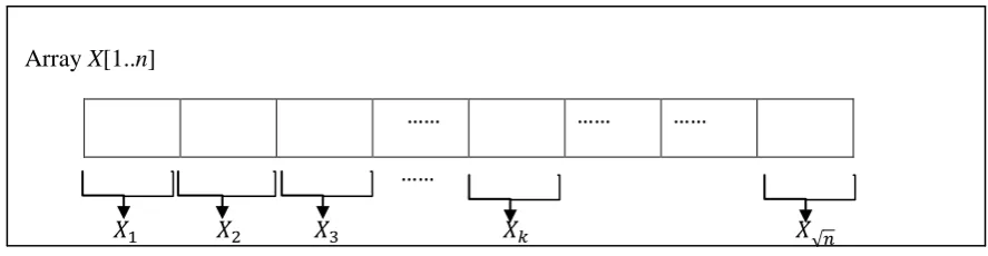
1. Given an array X with n data element indexed from 1 to n, one can view the array as consisting of

√

smaller adjacent arrays X[1..

√

], X[1+

√

..2

√

], …, X[n+1-

√

.. ] as shown in Figure 1. we shall refer to these sub-arrays as:

_√ .

2. Sort each sub-array , 1 ≤ i ≤

√

, using insertion sort.

3. For each element X[j], j = 1, 2, 3, …, n, of the array X, perform the following variant of Selection sort:

If X[j] falls in the sub-array , then for all sub-arrays … _√ perform selection of minimum of all of these sub-arrays as follows:

i. Find the minimum, and its location of only the first elements of each sub-array ii. Compare this minimum and the element X[j], and if this minimum is less then swap

with X[j], in which case we perform insertion sort iteration on the sub-array from which the element X[j] was moved to in order to make sure that the sub-array remains sorted.

Array

X

[1..

n

]

……

_√

Figure 1

Lemma 1. The hybrid technique sorts the array X in situ. Proof.

The correctness of the technique follows by induction:

The first position of the array X will hold the smallest of the elements in the first position of all the sub-arrays. Since each sub array was already sorted using insertion sort, it follows that the first position of each sub-array contains the smallest element in that sub-array and hence the first position of X will contain the smallest element in the whole array.

Now assume that we are currently in the j+1st iteration of step 3 and all the elements up to and including the jth element of array X are indeed the smallest j elements of the array and are in sorted order.

Let

⌈

√

⌉

be the value of the quotient of division of j+1 over

√

with the fraction rounded up to the next integer, and let

√

.

Thus the j+1st of the array X is also the ith element of the sub-array.

Step 3.i performs the operation of selection sort by finding the minimum of the elements in locations j+1..n. it does so by finding the smallest of the smallest element of the remaining sub-arrays

_√and comparing that smallest value with the current element in (j+1) position of the array X to place the smallest in that location. Thus location j+1 of the array X will hold the smallest j+1st element of the array after the iteration is completed.

(5)

Mirza Abdulla, International Journal of Computer Science and Mobile Applications,

Vol.3 Issue. 12, December- 2015, pg. 15-21

ISSN: 2321-8363

©2015, IJCSMA All Rights Reserved, www.ijcsma.com 19

From the discussion above one can see that we avoided the selection of the minimum of the unsorted data items in the array by selecting only the minimum element of the smallest value of the sub-arrays. Therefore, now we need only to inspect

√

elements of the array X to find the minimum of the remaining elements of the array. It is here where we gain the benefit of reducing the asymptotic time complexity of the classical Selection sort by a factor of

√

.

The Hybrid Algorithm

Given array X[1..n] of integer values

S# statement cost times

1 for i = 1 to

√

{ C1 1+

√

2 lb = (i-1)*

√

+1 C2

√

3 ub = (i)*

√

C3

√

4 InsertionSort (X [lb.. ub]) } C4

√ √

√

5 for i = 1 to n-1 { C5

6

⌈ √ ⌉

C6 -1

7 lb = j*

√

+1 C7 -1

8 min = X [lb] C8 -1

9 minj = lb C9

10 k = minj C10 -1

11 while (k <

√

) { C11

√

12 if X [k] < X [minj] C12

√

13 minj= k C13

√

14 k = k +

√

} C14

√

15 if X [minj] < X [lb] { C15

16 swap(X [k], X [minj]) C16

17 InsertionSort (X [minj .. minj - 1+

√

]) } C17

√

18 i=i+1 } C18

Analysis of the hybrid algorithm

.

Steps 1 to 4 of the algorithm sort the sub-arrays

_√ of the array X. each sub array consists

of only

√

data items. Thus step 4 would take C4*(

√

)2 to sort each sub array, from which it follows that the overall time for step 4 is C4*

√

. In steps 5 to 8 we iterate over the array X starting from the first data element up to the last. In step 6 we find the sub-array the current element belongs to, and steps 7 and 8 we find the lower and upper bounds of the next adjacent sub-array. In steps 9 to 15 we select the minimum of the remaining unsorted data items of X by only going thru the first element of each sub-array . We compare that element with item currently under consideration and swap the values if the current value in location j of the array X is not the minimum. In step 17 we make sure that the sub-array from which the swapped item came

(6)

Mirza Abdulla, International Journal of Computer Science and Mobile Applications,

Vol.3 Issue. 12, December- 2015, pg. 15-21

ISSN: 2321-8363

Note that the when steps 13 or 15 and 16 are performed the value of and

are equal to 1, and 0 otherwise. Thus we have as a worst case time complexity:

𝐶 𝐶 ( √ ) 𝐶 ( √ ) 𝐶 ( √ ) 𝐶

𝐶 𝐶 𝐶 𝐶 𝐶 𝐶 𝐶 𝐶 𝐶

√ 𝐶 𝐶 √ √ 𝐶 √

Rearranging we get

𝐶 𝐶 𝐶 𝐶 𝐶 𝐶 √

𝐶 𝐶 𝐶 𝐶 𝐶 𝐶 𝐶 𝐶 𝐶

𝐶 𝐶 𝐶 𝐶 𝐶 𝐶 √ 𝐶 𝐶 𝐶 𝐶 𝐶

𝐶 𝐶 𝐶 𝐶 𝐶 𝐶

Thus

√ √

Where

𝐶 𝐶 𝐶 𝐶 𝐶 𝐶

𝐶 𝐶 𝐶 𝐶 𝐶 𝐶 𝐶 𝐶 𝐶

𝐶 𝐶 𝐶 𝐶 𝐶 𝐶

And

𝐶 𝐶 𝐶 𝐶 𝐶 𝐶 𝐶 𝐶 𝐶 𝐶 𝐶

It follows therefore, that

√ √ √

giving the substantial improvement of a factor of

√

over the performance of either insertion sort or selection sort.

Best case performance of the Hybrid algorithm

The best case time complexity performance of the algorithm occurs when steps 13 or 15 and 16 are never executed the value of and

are then equal to 0. This occurs when the data in array X were already in required sorted order. In such a case step 4 would take

𝐶

time, and as mentioned earlier, steps 13, 15, and 16 are never executed. However, the complexity remains

√

since steps 11, 12, and 14 are executed that many times. This follows from the fact that Selection sort would perform

time in the best case too.

Thus we have:

Theorem. The Hybrid Selection Insertion algorithm best, average, and worst case performance are all

√

.

4. Conclusion

In this paper we presented an algorithm built using the ideas of classical selection and insertion sorting. We proved that the new hybrid algorithm has a worst, best, and average case time complexity of

√

. The idea was to reduce the time it takes selection sort to find the minimum element from

to just

√

.

This was achieved by

treating the input array as constituting of

√

sorted sub-arrays each of size

√

.

The use of sub-arrays reduced the time a data item is moved from its current position to its correct position from in the classical insertion sort technique to just

√

places in the hybrid technique.

References

[1]Anon., 1891, Untitled reports on Hollerith sorter, J. American Stat. Assoc. 2, 330-341

[2]Shaw M., 2003, Writing good software engineering research papers, In Proceedings of 25th International Conference on Software Engineering, pp.726-736

[3] Flores I. ,Oct 1960, "Analysis of Internal Computer Sorting". J.ACM 7,4, 389- 409.

[4] Knuth, D., 1998"The Art of Computer programming Sorting and Searching", 2nd edition, vol.3. Addison- Wesley. [5] Soubhik Chakraborty, Mausumi Bose, and Kumar Sushant, A Research thesis, On Why Parameters of Input

(7)

Mirza Abdulla, International Journal of Computer Science and Mobile Applications,

Vol.3 Issue. 12, December- 2015, pg. 15-21

ISSN: 2321-8363

[6] D.S. Malik, 2002, C++ Programming: Program Design Including Data Structures, Course Technology(Thomson Learning), www.course.com.

[7] J. L. Bentley and R. Sedgewick, 1997, "Fast Algorithms for Sorting and Searching Strings", ACM-SIAM SODA ‟97, 360-369.

[8] T. H. Cormen, C. E. Leiserson, R. L. Rivest, and C. Stein, 2001,."Introduction to Algorithms". MIT Press, Cambridge, MA, 2nd edition.

[9] Flores, I., Jan 1961, "Analysis of Internal Computer Sorting". J.ACM 8, 41-80.

[10] V.Estivill-Castro and D.Wood, 1992,"A Survey of Adaptive Sorting Algorithms", Computing Surveys, 24:441-476. [11] Cocktail Sort Algorithm or Shaker Sort Algorithm,

http://www.codingunit.com/cocktail-sort-algorithm-or-shaker-sort-algorithm.

[12] S. Jadoon, S. F. Solehria, S. Rehman and H. Jan, “Design and Analysis of Optimized Selection Sort Algorithm”, International Journal of Electric & Computer Sciences (IJECS-IJENS), vol. 11, no. 01, pp. 16-22.

[13] S. Chand, T. Chaudhary and R. Parveen, 2011, “Upgraded Selection Sort”, International Journal on Computer Science and Engineering (IJCSE), ISSN: 0975-3397, vol. 3, no. 4, pp. 1633-1637.

[14] J. Alnihoud and R. Mansi, 2010, “An Enhancement of Major Sorting Algorithms”, International Arab Journal of Information Technology, vol. 7, no. 1, pp. 55-62.

[15] O. O. Moses, 2009, “Improving the performance of bubble sort using a modified diminishing increment sorting”, Scientific Research and Essay, vol. 4, no. 8, pp. 740-744.

[16] H. W. Thimbleby, 1989, “Using Sentinels in Insert Sort”, Software-Practice and Experience, vol. 19, no. 3, pp. 303-307.

[17] T. S. Sodhi, S. Kaur and S. Kaur, 2013, “Enhanced Insertion Sort Algorithm”, International Journal of Computer Applications, vol. 64, no. 21, pp. 35-39.

A Brief Author Biography

Mirza Abdulla

– A full time faculty member of the Computer Science Department in the AMA International