http://www.sciencepublishinggroup.com/j/ajtas doi: 10.11648/j.ajtas.20190801.15
ISSN: 2326-8999 (Print); ISSN: 2326-9006 (Online)
Class of Difference Cum Ratio–Type Estimator in Double
Sampling Using Two Auxiliary Variables with Some Known
Population Parameters
Akingbade Toluwalase Janet, Okafor Fabian Chinemelu
Department of Statistics, Faculty of Physical Sciences, University of Nigeria, Nsukka, Nigeria
Email address:
To cite this article:
Akingbade Toluwalase Janet, Okafor Fabian Chinemelu. Class of Difference Cum Ratio–Type Estimator in Double Sampling Using Two Auxiliary Variables with Some Known Population Parameters. American Journal of Theoretical and Applied Statistics.
Vol. 8, No. 1, 2019, pp. 31-38. doi: 10.11648/j.ajtas.20190801.15
Received: February 2, 2019; Accepted: March 12, 2019; Published: April 1, 2019
Abstract:
In this paper, a class of double sampling difference cum ratio - type estimator using two auxiliary variables was proposed for estimating the finite population mean of the variable of interest. The expression for the bias and the mean square error of the proposed estimators are derived; in addition, some members of the class of the estimator are identified. The conditions under which the proposed estimators perform better than the sample mean and the existing double sampling ratio type estimators are derived. The empirical analysis showed that the proposed class of estimator performs better than the existing estimators considered in this study.Keywords:
Mean Square Error (MSE), Ratio Estimator, Double Sampling, Percent Relative Efficiency (PRE), Auxiliary Variables1. Introduction
Proper use of auxiliary variable is always known to improve the performance of estimators. Ratio, product and regression estimators are the most common and widely discussed in sampling theory literature. Ratio and product estimators are not as efficient as regression estimator except when the regression line passes through the origin. In real life situations, the line does not pass through the origin. This limitation has made many authors to provide alternatives to get better estimates. Authors like Kadilar and Cingi, [1, 2], Raja et al., [3], Sisodia and Dwivedi, [4], Singh and Kakran, [5], Singh and Tailor, [6], Subramani and Kumarapandiyan, [7], Upadhyaya and Singh, [8] and Yan and Tian [10] have modified the classical ratio estimator by Cochran [10]using some known population parameters like coefficient of variation, coefficient of skewness e.t.c. , of an auxiliary variable when the population mean of the auxiliary variable is known.
Sometimes it has been observed in sample surveys that information may be available on more than one auxiliary variable. Some authors like Kadilar and Cingi, [11], Mohanty, [12], Olkin, [13], Singh, [14] and Swain, [15], have worked on
the use of two auxiliary variables in the estimation of the population mean of the variable interest. In their work, they assumed that the population means of the two auxiliary variables are known. In real practical survey situation, the population means of the two auxiliary variables may not be available. In this condition it is customary to use two phase sampling or double sampling scheme for estimating the population means of the auxiliary variables, see Cochran [10]. In the literature, several authorshave proposed different estimatorsin double sampling for estimating the finite population mean of the study variable using two auxiliary variables. Authors like Mohanty, [12], Mukerjee et al., [16] and Muhammad et al., [17], suggested some estimators with an assumption that the population means of the two auxiliary variables are unknown.
Mohanty suggested regression ratio estimator indouble sampling ( ) using two auxiliary variables x and z, [12]. Which is given by
ˆ ( )
M yx
z
T y b x x
z ′
′
= + − (1)
(
)
ˆ
(
)
MRV yx yz
T
= +
y
b
x
′
−
x
+
b
z
′
−
z
(2)Muhammad et al. [17] also proposedregression type estimators by adopting Mohanty’s,[12] and Mukerjee et al, [16] estimators. The estimator is given by
ˆ ( ) (1 )
MNM yx
z z
T y b x x
z z
θ ′ θ
′
= + − + −
′
(3)
where θis suitably chosen constant. x′, z′are sample means based on the first phase sample; y x, , zare sample means based on the subsample.
(sample regression coefficient of y on x) , , (sample regression coefficient of x on z)
However, these authors did not consider the use of population parameters of any of the auxiliary variables like coefficient of variation, coefficient of skewness, decilese.t.c. to improve on the efficiency of the estimators. In this study, a class of difference cum ratio-type estimator in double sampling was proposed. Some known population parameters of one of the auxiliary variables were used to construct the estimator.
2. The Proposed Class of Ratio Estimator
Using Two Auxiliary Variables in
Double Sampling
Consider a finite population U =
{
u u1, 2,...uN}
of size N. Let Y bethe study variable andX, Zbe the two auxiliary variables, taking values(yi, xi, zi) on the ith unit of thepopulation. Let ( , , ̅) be the population means of (y, x, z), respectively. Suppose the population means of the auxiliary variables are unknown. In such a situation we use a two phase sampling. A preliminary large sample (n′)is selected using simple random sampling from N;information of the auxiliary variables are obtained from the sample. Information on the variable of interest (y) is collected from a second random sampleof size n is selected from the first phase sample (n <n′).
2.1. The Proposed Class of Estimator
Following Kadilar and Cingi, [1, 2] and Tripathi et al., [18], the proposed estimator is of the form:
(
)
1 *
2
( )
ˆ
( )
dp
y t x x Ax G
T
Ax G t z z α
γ γ
α
γ γ
− − ′ ′+
=
+ − − ′
(4)
A and G are assumed known function of the auxiliary variable X such as coefficient of kurtosis (β"(#)), coefficient of skewness(β$(#)), coefficient of variation (C# ), deciles (first decile, D$(#),second decile, D"(#), …, tenth decile), correlation coefficient between X and Y (ρ#*). Also0 < - ≤ 1,t$and t" are unknown constants. The scalar αtakes values -1, (for product-type estimator) and + 1 (for ratio-type estimator).
2.2. Derivation of the Bias and Mean Square Error of the Proposed EstimatorTˆdp*
To obtain the Bias and MSE of 12∗ , up to the first order of approximation, let us define
(1 x), (1 x) , (1 x) , (1 z)
x=X + ∆ x′=X + ∆′ x′γ =X + ∆′ γ z′γ =Z + ∆′ γ
(1 x)
xγ =Xγ + ∆ γ, zγ =Zγ(1+ ∆z)γ,y=Y(1+ ∆y) Expressing the proposed estimator 12∗ in terms of ∆′swe have
1 *
2
(1 ) (1 ) (1 )
ˆ
(1 ) (1 ) (1 )
Y X X X
dp
X Z Z
Y Y t X X AX G
T
AX G t Z Z
α
γ γ γ γ
α
γ γ γ γ
+ ∆ − + ∆ − + ∆′ + ∆′ +
=
+ ∆ + − + ∆ − + ∆′
(5)
Expanding (5) to the first order of approximation using binomial series expansion, stopping at order 2, we have
2 2
* 1 1 1 1
1 1 1 1
2 2
2 2 2 2 2 2
1 1 1 1
2
2 2 1 2 1 2 1 2 1 2 2 2
( 1) ( 1)
ˆ
2 2
( 1) 2
X X
dp Y X X X X Y
X Z
X X Y X X X X
Z Y X Z X Z X Z
t q t q
T Y Y t q t q Y Y
Y t q Y
Y Y t q t q Y
K
t q Y t t q q t t q q t q Y
K K K K
γ γ αλ αλ
α α λ αλ αλ αλ αλ α λ α
α α α α λ
′
− ∆ ′ − ∆ ′ ′
= + ∆ − ∆ − + ∆ + + ∆ + ∆ ∆
′
− ∆ ′ ′ ∆
+ − ∆ − ∆ ∆ + ∆ − ∆ − ∆ ∆ +
′ ′
∆ ∆ ∆ ∆ ∆ ∆ ∆ ∆
+ − + +
2
2 2 2 2 2 2 1 2 1 2 1 2 1 2
2 2 2 2 2 2 2
2 2 2 2 2 2
2
2 2 2
2 2 2 2 2 2
2
( 1) 2
( 1) ( 1) ( 1)
2 2 2
( 1) ( 1) ( 1)
2
Z Z Z Y X Z X Z
X Z Z X Z
Z X Z X Z
t q Y t q Y t q Y t t q q t t q q
K K K K K
t q Y t q Y Y t q Y
K K K
t q Y t q Y t q Y
K K
K
α γ α α α α
α λ α γ α α λ α α
α α α α λ α α λ
′ ′ ′ ′ ′
− ∆ ∆ ∆ ∆ ∆ ∆ ∆ ∆
+ − − + − −
′ ′ ′
∆ ∆ − − ∆ + + ∆ + + ∆ +
′ ′
+ ∆ − + ∆ ∆ + + ∆ ∆ 2 2 2
2 2 2
( 1)t q Y Z K α α+ ∆′ −
1 , 2 ,
q =γXγ q =γZγ K =AX+G, AX
AX G λ=
+
Taking expectation of (6) and using the results:
E7∆ 8 = E(∆:) = E(∆;<) = E(∆:<) = E(∆;) = 0
=(∆>") = ?$@>", =(∆:") = ?$@:", =(∆") = ?$@;" , =7∆:<
A
8 = =(∆:∆:<) = ?"@:"
=7∆;<A8 = ?
"@;",=(∆:>< ) = ?"B @:@>, =(∆:<∆;) = ?"B:;@:@;
=(∆:∆;) = ?$B:;@:@; , =(∆;<∆>) = ?"B;>@;@>,=(∆ ∆>) = ?$B;>@;@>
1 2
1 1 1 1
,
n N n N
ω = − ω = ′− , 3 1 1
n n ω = − ′
After simplification, the bias is
*
ˆ
B(Tdp)=E T(ˆdp* −Y)=
2 2 2
2 2
2
1 1
1 1
3 2 2 2 2
1 2 1 2 2 2 2 2 2 2
2
( 1) ( 1)
2 2
( 1)
( 1) ( 1)
2 2
zy z y
x x
xy x y x
xz x z z z xz x z
t q Y C C
t q C YC
Y C C t q C
K
t t q q C C t q YC t q YC t q Y C C
K K K K
α ρ
γ αλ ρ α α λ αλ
ω
α ρ α γ α α α α λ ρ
− +
− − + + + −
− + +
+ + −
(7)
The mean square error of this estimator is
* * 2
ˆ ˆ
( dp) ( dp ) MSE T =E T −Y
Which from (6) and ignoring order higher than 2 and after simplification we have
2 2 2 2 2
* 2 2 2 2 2 2 2 2 2 2 2
1 3 1 1 2 1 1
2 2 2
2 2
2 2 1 2 1 2 2 2
1 1
ˆ
MSE( ) [ 2{
}] z
dp y x x xy x y
zy z y xz x z xz x z
xy x y x
t q Y C
T Y C t q C Y C t q Y C C
K
t q Y C C t t q q Y C C t q Y C C
Y C C t q YC
K K K
α
ω ω α λ ρ
α ρ α ρ α λ ρ
αλ ρ αλ
= + + + −
+ − − + +
(8)
In order to obtain the optimum values of t1and t2we differentiate (8) simultaneously with respect to t1and t2and solve the resultant equations. This gives
0
2
1
1 2
1
( ) (1 )
(1 )
y xy xz zy x xz
x xz
YC YC l
t Y
q X Cγ
ρ ρ ρ αλ ρ αλ
γ ρ
− − − −
= =
−
(
)
0
2
2 2
2
( )
(1 )
y zy xy xz
z xz
C AX G l K
t
q Z Cγ
ρ ρ ρ
α
αγ ρ
− +
= − = −
−
Where 1 2
( )
and
(1 )
y xy xz zy
x xz
YC l
C
ρ ρ ρ
ρ
− =
− 2 2
( )
(1 )
y zy xy xz
z xz
C l
C
ρ
ρ ρ
ρ
− =
−
Substituting the optimum values t1o and t2oin (8) we obtain the minimum mean square error
* 2 2 2 2 2 2
1 3 1 2 1 2 1 2
ˆ
MSE(Tdp opt) =Y [
ω
Cy+ω
{l Cx+l Cz −2(lρ
xyC Cx y+lρ
zyC Cz y−l lρ
xzC Cx z)}] (9)3. Sub-members of the Proposed Class of
Ratio-type Estimator
Settingt t1, , ,2 α γ, A and G to specific values in (4), some
estimators which can be regarded as members of this
proposed estimator can be obtained. For instance, if
1 0
t = =α we have the usual sample mean estimator.
Also setting
C$= =DDEF
E
A(sample regression coefficient of y on x) , C"=
=DEG
DGA,(sample regression coeffcient of x on z), where
2
x
and s2z are thesample variances of x and z respectively, sxy and sxz are the sample covariances between x and y and between x and z, respectively and H = 1 (ratio estimator), we have a member of the class of ratio-type regression estimator for estimating the population mean using two auxiliary variables when the population mean of two auxiliary variables are unknown presented below.
(
)
* ( )
ˆ
( )
xy dp
xz
y b x x Ax G
T
Ax G b z z
γ γ
β γ γ
− − ′ ′+
=
+ − − ′
, 0 < - ≤ 1 (10)
Using the large sample approximation as used in the case of the regression estimation of the population mean, where
2
tends to
xy xy xy x
b
β
=S S and bxz tends to βxz=Sxz Sz2 ,the bias and mean square error, from (7) and (8) are as follows:
1 1 2 2
* 2 2
3 1 1
2 2 2 2 2 2 2
1 2 2 2 2 2 2 2 2
2
( 1) ˆ
B( ) [
2
( 1) 2
] 2
xy x y xz zy x y
dp xy x y x xy x y
xy xz x y xz x z xz x xz x
q R Y C C q R Y C C
T Y C C YC q R C C
K
q q R Y C C q R Y C C q R Y C q R Y C
K K K K
β
ω
γ
ρ
λ ρ
λ
λ
ρ
ρ ρ
ρ ρ
γ
ρ
ρ
λ
ρ
−
= − − + + +
−
− + + − (11)
2 2 2 2 2
* 2 2 2 2 2 2 2 2 2 2 2 2 2
1 3 1 1 2 1 1
2 2 2 2
2 2 1 2 1 2
2 2 2
1 1
ˆ
MSE( ) [ 2{
}] xz z
dp y xy y x xy y
xz zy y xy xz x y xz x
xy x y xy x y
R q Y C
T Y C R q C Y C R q Y C
K
R q Y C Cx R R q q Y C C R q Y C
Y C C R q Y C C
K K K
β
ω
ω
ρ
λ
ρ
ρ
ρ ρ
ρ ρ
λ
ρ
λ ρ
λ
ρ
= + + + −
+ − − + +
(12)
Where R1=Y X, R2 =X Z . If weset R q1 1=q3 and q4 =R q2 2 K, equation (12) becomes
* 2 2 2 2 2 2 2 2 2 2 2 2 2 2
1 3 3 4 3
2 2 2 2 2
4 3 3 4 4
ˆ
MSE( ) [ 2{
}]
dp y xy y x xz z xy y
xy x y xz zy y xy x y xy xz x y xz x
T Y C q C Y C q Y C q Y C
Y C C q Y C Cx q Y C C q q Y C C q Y C
β ω ω ρ λ ρ ρ
λ ρ ρ ρ λ ρ ρ ρ λ ρ
= + + + −
+ − − + + (13)
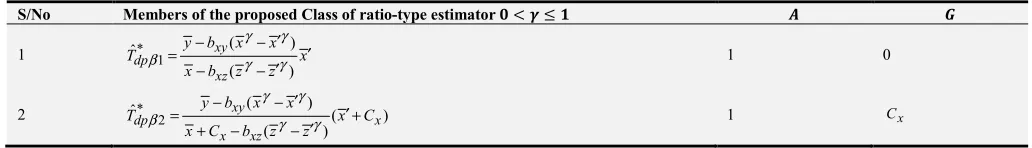
Estimators in this class of ratio type regression estimator are found in Table 1.
4. Theoretical Comparison of the
Proposed Estimator with Other
Existing Estimators Discussed
In this section, the performance of the proposed estimator
with other existing estimators were compared, through their mean square errors, like the sample mean, Tˆ0 =y , with variance V T(ˆ0)=
ω
1Y C2 y2, the estimator ˆTMby Mohanty, [12] found in (1); the estimators ˆTMRV by Mukerjee, [16] found in (2) and the estimator ˆTMNMby Muhammad[17] found in (3).The mean square errors of these existing estimators are:
2 2 2 2 2 2 2 2
1 3
ˆ
( M) { y ( xz z ( xy y xz z) ( z yz y) y yz}
MSE T =Y
ω
C +ω ρ
C −ρ
C −ρ
C + C −ρ
C −Cρ
(14)2 2 2 2
1 3
ˆ
( MRV) y{ ( xy yz 2 xy xz yz)}
MSE T =Y C
ω ω ρ
− +ρ
−ρ ρ ρ
(15)and
2 2 2 2
1 3
ˆ
( MNM) y{ ( xy ( yz xy xz) )}
MSE T =Y C
ω ω ρ
− +ρ
−ρ ρ
(16)The performance of the proposed estimator using the minimum MSE in (9) and MSE of the existing estimators presented in (14), (15) and (16).
The proposed estimatorTˆdp* is better, in terms of having smaller MSE, than the sample mean if and only if from (9)
*
ˆ ˆ
( dp opt) ( o) MSE T ≤V T iff
2 2 2 2
1 x 2 z 2(1 xy x y 2 zy z y 1 2 xz x z)
l C +l C ≤ l
ρ
C C +lρ
C C −l lρ
C C2 2 2 2 2 2 2 2 2 2
1 x 2 z 2(1 xy x y 2 zy z y 1 2 xz x z) 3( xz z ( xy y xz z) ( z yz y) y yz
l C +l C − l
ρ
C C +lρ
C C −l lρ
C C ≤ω ρ
C −ρ
C −ρ
C + C −ρ
C −Cρ
The proposed estimator Tˆdp* will be more efficient than the existing estimator ˆTMRVby Mukerjee et al., [16]. Using (9) and (15),MSE T(ˆdp opt*) ≤MSE T(ˆMRV)
iff
2 2 2 2 2 2
1 x 2 z 2(1 xy x y 2 zy z y 1 2 xz x z) ( xy yz 2 xy xz yz)
l C +l C − l
ρ
C C +lρ
C C −l lρ
C C ≤ −ρ
+ρ
−ρ ρ ρ
From (9) and (16) the proposed estimatorTˆdp* will be better than the existing estimator ˆTMNM by Muhammad et al., [17] iffMSE T(ˆdp opt* ) ≤MSE T(ˆMNM)
which is equivalent to
2 2 2 2 2 2
1 x 2 z 2(1 xy x y 2 zy z y 1 2 xz x z) ( xy ( yz xy xz) )
l C +l C − l
ρ
C C +lρ
C C −l lρ
C C ≤ −ρ
+ρ
−ρ ρ
Now comparing these estimators Tˆdp* andTˆdp*βusing (9) and (13), estimatorTˆdp* will be more efficient than Tˆdp*βiff
{
}
(
)
{
}
{
}
2 2 2 2 2 2 2 2 2 2
1 4 2 4 3
2 2 2
3 1 3 4 4 2 1 2
( ) ( ) 2
2 ( ) 2
xz x xz z xy y
xy y x xy x y zy x y zy z y xz x z
Y l q C l q C Yq C
q C YC C C Y l Yq q Y q C C l C C l l C C
λρ
ρ
ρ
ρ
λ
ρ
λ
ρ
ρ
ρ
+ + − +
≤ + − − + + + −
5. Empirical Comparison
In this section, the mean square errors, and percent relative efficiencies (PREs) of the existing and the proposed estimators with respect to the sample mean ˆTo were computed. The results are given in Tables 2 and 3. Real life
data set by Chattefuee and Hadi,[19] and details of the data are as shown below:
Y-Per capita expenditure on education in 1975
- Per capita income in 1973
− Number of residents per thousand living in urban areas in 1970
J = 50 L<= 35 L = 15 = 284.0612 = 4675.12 ̅ = 657.8
B = 0.60679 B = 0.31675 B = 0.61937 U = 733.1407 = 0.058228 = 2.764116 = 0.13756 @ = 0.21776 @ = 0.13786 @ = 0.2204 V$( )= 3817 V"( )= 3967 VW( )= 4243 VX( )= 4504 VY( )= 4697
VZ( )= 4827 V[( )= 4989 V\( )= 5309 V]( )= 5560 V$^= 5889
_"= −0.94843 _$= 0.05675
The Percent Relative Efficiencies (PREs) of the existing estimators mentioned in (1), (2)and (3) and the jth members of the proposed estimators ˆ*
j
dp
T β , j=1, 2, 3,…, 20 given in Table 1andTˆdp* (for minimum variance in (9)) with respect to the usual sample mean `, is of the form;
PRE =abc(def)
gh(.) ∗ 100where (.) = ˆTM or ˆTMRVor ˆTMNMor the
proposed estimator.
The higher the percent relative efficiencies, the more efficient the estimator.
Table 1. Members of the proposed class of double sampling ratio estimator using two auxiliary variables.
S/No Members of the proposed Class of ratio-type estimator i < j ≤ k l m
1 ˆ* 1 ( )
( )
xy dp
xz
y b x x
T x
x b z z
γ γ
β = − γ − ′γ ′ ′
− − 1 0
2 ˆ* 2 ( ) ( )
( )
xy
dp x
x xz
y b x x
T x C
x C b z z
γ γ
β = − −γ ′ γ ′+ ′
S/No Members of the proposed Class of ratio-type estimator i < j ≤ k l m
3 * 3 2( )
2( )
( )
ˆ ( )
( )
xy
dp x
x xz
y b x x
T x
x b z z
γ γ
β γ γ β
β ′ − − ′ = + ′
+ − − 1 β2( )x
4 * 4 2( )
2( )
( )
ˆ ( )
( )
xy
dp x x
x x xz
y b x x
T x C
x C b z z
γ γ
β = β − − ′γ ′γ ′β +
+ − − β2( )x Cx
5 * 5 2( )
2( )
( )
ˆ ( )
( )
xy
dp x x
x x xz
y b x x
T x C
xC b z z
γ γ
β γ γ β
β ′ − − ′ = + ′
+ − − @ _"( )
6 * 6
( )
ˆ ( )
( )
xy
dp xy
xy xz
y b x x
T x
x b z z
γ γ
β = ρ− −γ ′ ′γ ′+ρ
+ − − 1 ρxy
7 ˆ* 7 ( ) ( )
( )
xy
dp x xy
x xy xz
y b x x
T x C
xC b z z
γ γ
β = +−ρ − −γ′− ′γ ′ +ρ Cx ρxy
8 * 8
( )
ˆ ( )
( )
xy
dp xy x
xy x xz
y b x x
T x C
x C b z z
γ γ
β = ρ − −γ′ γ ′ρ +
′
+ − − B @
9 * 9 2( )
2( )
( )
ˆ ( )
( )
xy
dp x xy
x xy xz
y b x x
T x
x b z z
γ γ
β = β −ρ − ′γ ′γ ′β +ρ
+ − − _"( ) B
10 * 10 2( )
2( )
( )
ˆ ( )
( )
xy
dp xy x
xy x xz
y b x x
T x
x b z z
γ γ
β γ γ ρ β
ρ β ′ − − ′ = + ′
+ − − B _"( )
11 * 11 1( )
1( )
( )
ˆ ( )
( )
xy
dp x
x xz
y b x x
T x D
x D b z z
γ γ
β = − −γ′ ′γ ′+
+ − − 1 V$( )
12 * 12 2( )
2( )
( )
ˆ ( )
( )
xy
dp x
x xz
y b x x
T x D
x D b z z
γ γ
β = + − − −γ′− ′γ ′+ 1 V"( )
13 * 13 3( )
3( )
( )
ˆ ( )
( )
xy
dp x
x xz
y b x x
T x D
x D b z z
γ γ
β = − −γ′ γ ′+
′
+ − − 1 VW( )
14 * 14 4( )
4( )
( )
ˆ ( )
( )
xy
dp x
x xz
y b x x
T x D
x D b z z
γ γ
β = − −γ′ ′γ ′+
+ − − 1 VX( )
15 * 15 5( )
5( )
( )
ˆ ( )
( )
xy
dp x
x xz
y b x x
T x D
x D b z z
γ γ
β = − −γ′ γ ′+
′
+ − − 1 VY( )
16 * 16 6( )
6( )
( )
ˆ ( )
( )
xy
dp x
x xz
y b x x
T x D
x D b z z
γ γ
β = − −γ′ ′γ ′+
+ − − 1 VZ( )
17 * 17 7( )
7( )
( )
ˆ ( )
( )
xy
dp x
x xz
y b x x
T x D
x D b z z
γ γ
β = + − − −γ′− ′γ ′+ 1 V[( )
18 * 18 8( )
8( )
( )
ˆ ( )
( )
xy
dp x
x xz
y b x x
T x D
x D b z z
γ γ
β = − −γ′ γ ′+
′
+ − − 1 V\( )
19 * 19 9( )
9( )
( )
ˆ ( )
( )
xy
dp x
x xz
y b x x
T x D
x D b z z
γ γ
β = − −γ′ ′γ ′+
+ − − 1 V]( )
20 * 20 10( )
10( )
( )
ˆ ( )
( )
xy
dp x
x xz
y b x x
T x D
x D b z z
γ γ
β = − −γ′ γ ′+
′
+ − − 1 V$^( )
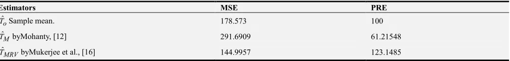
Table 2. The MSE and PRE with respect to ^ of the existing and proposed estimators.
Estimators MSE PRE
ˆ
o
T Sample mean. 178.573 100
ˆ
M
T byMohanty, [12] 291.6909 61.21548
ˆMRV
Estimators MSE PRE
ˆMNM
T by Muhammad et al., [17] 124.3938 143.5441
The proposed estimator(Tˆdp opt*) 124.076 143.91
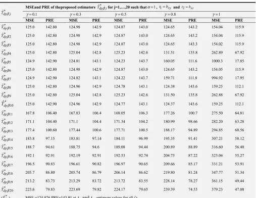
Table 3. The MSE and PREwith respect to ^ of the proposed estimators.
*
ˆ
dp j
T β
MSEand PRE of theproposed estimators Tˆdp j*β for j=1,…,20 such thatα=1, t1=bxy and t2=bxz
0.1
γ= γ=0.3 γ=0.5 γ=0.8 γ=1
MSE PRE MSE PRE MSE PRE MSE PRE MSE PRE
* 1
ˆ
dp
T β 125.0 142.80 124.98 142.9 124.87 143.0 124.65 143.2 154.04 115.9
* 2
ˆdp
T β 125.0 142.80 124.98 142.9 124.87 143.0 124.65 143.2 154.04 115.9
* 3
ˆ
dp
T β 125.0 142.80 124.98 142.9 124.87 143.0 124.65 143.3 154.02 115.9
* 4
ˆ
dp
T β 125.0 142.80 125.04 142.8 125.23 142.6 131.51 135.8 262.89 67.92
* 5
ˆ
dp
T β 124.9 142.90 124.81 143.1 124.23 143.7 160.05 111.6 1000.3 17.85
* 6
ˆ
dp
T β 125.0 142.80 124.98 142.9 124.87 143.0 124.65 143.2 154.05 115.9
* 7
ˆdp
T β 124.9 142.90 124.82 143.1 124.22 143.7 159.71 111.8 994.92 17.95
* 8
ˆ
dp
T β 125.0 142.80 124.96 142.9 124.78 143.1 124.38 143.6 159.25 112.1
* 9
ˆ
dp
T β 125.0 142.80 125.04 142.8 125.23 142.6 131.50 135.8 262.88 67.92
* 10
ˆ dp
T β 125.0 142.90 124.96 142.9 124.77 143.1 124.37 143.6 159.25 112.1
* 11
ˆ
dp
T β 167.8 106.40 167.83 106.4 168.05 106.3 177.26 100.7 275.50 64.81
* 12
ˆ
dp
T β 171.1 104.40 171.1 104.4 171.34 104.2 180.99 98.66 282.20 63.28
* 13
ˆ
dp
T β 177.4 100.60 177.44 100.6 177.71 100.5 188.17 94.89 294.85 60.56
* 14
ˆdp
T β 183.8 97.15 183.81 97.14 184.11 96.99 195.35 91.41 307.21 58.12
* 15
ˆ
dp
T β 188.7 94.61 188.75 94.6 189.08 94.44 200.89 88.89 316.60 56.40
* 16
ˆ
dp
T β 192.1 92.91 192.19 92.91 192.53 92.74 204.73 87.22 323.04 55.27
* 17
ˆ
dp
T β 196.5 90.83 196.61 90.82 196.97 90.65 209.66 85.17 331.21 53.91
* 18
ˆ
dp
T β 205.7 86.80 205.74 86.79 206.14 86.62 219.80 81.24 347.77 51.34
* 19
ˆdp
T β 213.2 83.73 213.29 83.72 213.72 83.55 228.14 78.27 361.15 49.44
* 20
ˆ
dp
T β 223.6 79.83 223.69 79.82 224.17 79.65 239.59 74.53 379.23 47.08
*
ˆ
(Tdp opt) MSE =124.076 PRE=143.91 at t1 and t2 optimum values for all j’s
6. Results and Discussion
6.1. Table 2 Results
The existing estimators ˆTMRV by Mukerjee et al.,[16] and estimator TˆMNM by Muhammad et al.,[17]for estimating the population mean of the study variable have significant improvement on the sample mean because they have smaller MSE and higher percent relative efficiency. The proposed estimator (Tˆdp opt*) is the most efficient estimator.
6.2. Table 3 Results
All the proposed estimators Tˆdp j*β , j=1,…,13 at 0.1 0.5
γ
= − , are more efficient than the sample meanbecause they have smaller MSE and higher percent relative efficiency while these proposed estimators Tˆdp j*β , j=14,…,20at
γ
=0.1 1− have no significant improvement on the sample mean because they have higher MSE and lower percent relative efficiency. The proposed estimators Tˆdp j*β , j=1,…,10 atγ
=0.1 0.5− are the most efficient estimators because they perform better than the sample mean, the existing estimators, ˆTM by Mohanty [12] and estimator,ˆ MNM
T by Muhammad et al.,[17]. The proposed estimators
*
ˆ dp j
that utilize the third to tenth deciles and they do not have significant improvement on the existing estimators.
In general, from Table 3 results, The proposed class of ratio type estimatorTˆdp* , att$and t" optimum values, is the most efficient estimator because it has the least MSE and the highest PRE and it slightly perform better than the existing estimators, ˆTMNMby Muhammad et al., [17]. Alternatively, a good guess of - for the sub-members,Tˆdp j*β , j=1,…,10, when
1 xy
t =b and t2 =bxz at
γ
=0.1 0.5− are efficient as estimator*
ˆ dp j
T β , j=1,…,20 att1and t2 optimum values.
7. Conclusion
In this work, a class of double sampling difference cum ratio-type estimator was proposed using two auxiliary variables with known population parameters of the auxiliary variable(X). The conditions under which the proposed estimators have minimum mean square errors are mentioned in section 4. In conclusion, the proposed class of double sampling ratio type estimator Tˆdp* att$and t" optimum values and sub-members of the proposed class of estimatorTˆdp j*β , j=1,…,10 at
γ
=0.1 0.5− performs better than the existing estimators by Mohanty, [12], Mukerjee et al., [16] and Muhammad et al., [17]. The proposed class of double sampling ratio type estimator is recommended for practical application.Acknowledgements
The authors are thankful to the anonymous learned referees for their constructive comments that led to the improvement of the paper.
References
[1] Kadilar, C. & Cingi, H. (2004), Ratio estimators in simple random sampling’, Applied Mathematics and Computation 151(3), 893–902.
[2] Kadilar, C. &Cingi, H. (2006), An improvement in estimating the population mean by using the correlation coefficient. Hacettepe Journal of Mathematics and Statistics 35(1), 103– 109.
[3] Raja, T. A., Subair, M., Maqbool, S. &Hakak, A.(2017) Enhancing the Mean Ratio Estimator for Estimating Population Mean Using Conventional Parameters; International Journal of Mathematics and Statistics Invention (IJSM)5(1),58-61.
[4] Sisodia, B. V. S. &Dwivedi, V. K.(1981) ‘A modified ratio estimator using coefficient of variation of auxiliary variable Journal of the Indian Society of Agricultural Statistics 33(1),13–18.
[5] Singh, H. P. & Kakran, M. S. (1993).: A modified ratio estimator using known coefficient of kurtosis of an auxiliary character. Revised version submitted to Journal of Indian Society of Agricultural Statistics, New Delhi, India.
[6] Singh, H. P. & Tailor, R. (2003), Use of known correlation coefficient in estimating the finite population means Statistics in Transition 6(4), 555–560.
[7] Subramani, J. &Kumarapandiyan, G.(2013)Estimation Of Finite Population Mean Using Decilesof an Auxiliary VariableStatistics in Transition-new series, Spring 2013 Vol. 14, No. 1, pp. 75–88.
[8] Upadhyaya, L. N. & Singh, H.(1999) Use of transformed auxiliary variable in estimating the finite population mean Biometrical Journal 41(5), 627–636.
[9] Yan, Z. &Tian, B., (2010). Ratio Method to the Mean Estimation Using Coefficient of Skewness of Auxiliary Variable, ICICA 2010, Part II, CCIS 106, pp. 103-110. [10] Cochran W. G. (1977), Sampling Techniques, 3rd edition,
Wiley Eastern Limited, New York.
[11] Kadilar, C., &Cingi, H. (2005). A new estimator using two auxiliary variables. Applied Mathematics and Computation, 162, 901-908.
[12] Mohanty, S.,(1967) Combination of regression and ratio estimate. J. Ind. Statist., 5:16-19.
[13] Olkin, I. (1958). Multivariate ratio estimation for finite populations. Biometrika, 45: 154-165.
[14] Singh, M. P. (1965). On the estimation of ratio and product of population parameters, Sankhya, Series C, 27, 321-328. [15] Swain A. K. P. C. (2012), On Classes Of Modified Ratio Type
and Regression-Cum-RatioTypeEstimators In Sample Surveys Using Two Auxiliary Variables Statistics In Transition-New series, Vol. 13, No. 3, pp. 473—494.
[16] Mukerjee, R., Rao T. J., &Vijayan, K., (1987), Regression type estimators using multiple auxiliary information. Austral. J. Statist., 29(3):244-254.
[17] Muhammad, H., Naqvi, H. & Muhammad Q. S., (2010)Some new regression type estimators in two phase sampling, World Applied Science Journal., 8(7):799-803.
[18] Tripathi, T. P., Das, A. K. & Khare, B. B., (1994). ‘Use of Auxiliary Information in Sample Surveys-A Review’ Aligarh Journal of Statistics, 14, 79-134.