R E S E A R C H A R T I C L E
Open Access
The appropriateness of Bland-Altman
’
s
approximate confidence intervals for limits
of agreement
Gwowen Shieh
Abstract
Background:Percentiles are widely used as reference limits for determining the relative magnitude and substantial importance of quantitative measurements. An important application is the advocated Bland-Altman limits of agreement.
Methods:To contribute to the data analysis and design planning of reference limit or percentile research, the purpose of this paper is twofold. The first is to clarify the statistical features of interval estimation procedures for normal percentiles. The second goal is to provide sample size procedures for precise interval estimation of normal percentiles.
Results:The delineation demonstrates the theoretical connections between different pivotal quantities for obtaining exact confidence intervals. Moreover, the seemingly accurate approximate methods with equidistant from the principal estimators are shown to have undesirable confidence limits. It is found that the optimal sample size has a minimum for median or mean, and increases as the percentile approaches the extremes.
Conclusions:The exact interval procedure should be used in preference to the approximate methods. Computer algorithms are presented to implement the suggested interval precision and sample size calculations for planning percentile research.
Keywords:Assurance probability, Expected width, Precision, Quantile, Sample size
Background
A percentile is a numerical measure that represents the reference point below which a given percentage of values in the target population fall. Because of the conceptual simplicity and context-free feature, percentiles are widely used for determining the relative magnitude and substantial importance of quantitative measurements in all scientific fields. For example, the children health conditions are often assessed by their weight and height in comparison to the national averages and percentiles found in the growth charts. Also, reference limits are extensively applied in medicine and related fields to iden-tify informative range of measurement from a reference population. The most typical reference limits contain the central 95% of the values in the population of interest. As an important application, the Bland and Altman [1, 2] 95% limits of agreement are comprised of the 2.5th
percentile and 97.5th percentile for the distribution of the difference between paired measurements.
The practical usage of percentiles is often represented by referring to a normal distribution. In this prominent case, the normal percentile is a linear function of the mean and standard deviation of the designated popula-tion. Note that the sample mean and sample variance are complete and sufficient statistics for the population mean and variance. Although estimation of normal percentile is not discussed in most standard texts, it is straightforward to obtain the minimum variance unbiased estimator of a normal percentile. However, the dominance property does not extend to other principles in decision theoretic analyses such as the mean square error criterion. Among others, Royston and Mathews [3] conducted a comparison of potential point estimators of normal percentiles with respect to bias and mean square error. More advanced and theoretical investigations of normal percentile estimators can be found in Keating,
Correspondence:[email protected]
Department of Management Science, National Chiao Tung University, Hsinchu 30010, Taiwan, Republic of China
Mason, and Balakrishnan [4], Keating and Tripathi [5], Parrish [6], Rukhin [7], and Zidek [8,9].
In view of the stochastic nature in statistical inference, it is more informative to construct confidence intervals for the target parameters than to provide a single esti-mate about their values. General expositions and com-prehensive guidelines of interval estimation are available in Hahn [10,11], Hahn and Meeker [12], and Vardeman [13]. Accordingly, various interval methods of normal percentiles have been described from different perspec-tives. The exact interval procedure of normal percentiles has been documented in the literature, for example, see Hahn and Meeker [12], Johnson, Kotz, and Balakrishnan [14], and Owen [15]. Moreover, the one-sided confi-dence intervals of normal percentiles have a close link to the one-sided tolerance bounds of a normal distribution as noted in David and Nagaraja [16], Krishnamoorthy and Mathew [17], and Odeh and Owen [18].
Notably, Bland and Altman [1, 2] suggested the 95% limits of agreement for evaluating the differences between measurements by two methods. The endpoints of the Bland-Altman 95% limits of agreement are the 2.5th percentile and 97.5th percentile for the distribution of the difference between paired measurements. To reflect the uncertainty due to sampling error, approximate inter-val formulas were presented for estimating the two indi-vidual percentiles. The large number of citations revealed that the Bland-Altman analysis has become the major technique for assessing agreement between two methods of clinical measurement. But the recent work of Carkeet [19] and Carkeet and Goh [20] provided detailed discus-sions in favor of exact confidence interval over the ap-proximate procedure considered in Bland and Altman [1, 2], especially when the sample sizes are small. Further considerations and reviews of measuring agreement in method comparison studies are available in Barnhart, Ha-ber, and Lin [21], Choudhary and Nagaraja [22], and Lin et al. [23].
Although the practical implementation of the exact inter-val procedure is well presented in Carkeet [19], the explica-tion of the differences between the exact and approximate methods mainly concentrated on the relative magnitudes and symmetric/asymmetric bounds of the resulting confi-dence limits. On the other hand, the endpoints of the Bland-Altman 95% limits of agreement are usually viewed as a pair of bound for measuring agreement in method comparison studies. Accordingly, Carkeet [19] and Carkeet and Goh [20] focused on the comparison of the approxi-mate confidence intervals for upper and lower limits of agreements as a pair and the exact two-sided tolerance intervals for a normal distribution. Therefore, the distinctive advantage of the exact interval procedures and the potential limitation of the approximate confidence intervals for the individual upper and lower limits of agreement were not
fully addressed in Carkeet [19] and Carkeet and Goh [20]. It is of practical importance to conduct a detailed appraisal of the accuracy and discrepancy between the exact and approximate interval procedures for an individual limit of agreement under a wide range of model configurations. The problem of obtaining a single confidence interval to cover both limits of agreement simultaneously is more involved and a detailed discussion of this topic is beyond the scope of the present study.
In addition to the abovementioned studies, a numerical comparison of several interval estimation methods of normal percentiles was presented in Chakraborti and Li [24]. They adopted a standardized minimum variance unbiased estimator as the pivotal quantity and proposed both exact and approximate confidence intervals of nor-mal percentiles. Their simulation study showed that the expected width and coverage probability of the suggested exact and approximate methods are nearly identical to that of the procedure described in Lawless ([25], p. 231). Despite the analytic arguments and empirical findings in Chakraborti and Li [24], the following two attentions to-ward their illustration should be noted. First, although it was demonstrated that Lawless’s [25] confidence intervals are the same as the existing formulas in Owen [15] and Odeh and Owen [18], they did not discuss the theoretical implications between their exact method and the estab-lished exact procedure. Second, in contrast to the asym-metry of the exact confidence intervals, the approximate confidence intervals of Chakraborti and Li [24] are equi-distant around the minimum variance unbiased estimate. Note that the two endpoints of a two-sided confidence interval can also be interpreted as the limits of one-sided confidence interval. Thus, the performance of the two limits of Chakraborti and Li’s [24] approximate interval method should be further evaluated with respect to the equal-tailed property. The analytic and numerical results in Chakraborti and Li [24] are not detailed enough to clar-ify these fundamental issues. It is prudent to elucidate these vital aspects of their methods to be accepted as a feasible technique.
magnitude of expected width, and the assurance prob-ability of interval width within a designated threshold. In view of the general availability of statistical software packages SAS and R, computer algorithms are developed to facilitate the implementation of the suggested confi-dence interval and sample size computations.
Methods
Assume X1, …, XN are a sample from a N(μ, σ2) population with unknown meanμand varianceσ2forN> 1. The sample meanX and sample varianceS2are defined as X ¼PNi¼1Xi=N and S2¼PNi¼1ðXi−XÞ
2
=ðN−1Þ , respectively. The 100pth percentile of the distribution N(μ,σ2) is denoted byθ, where
θ¼μþzpσ ð1Þ
and zp is the 100pth percentile of the standard normal
distribution N(0, 1). To estimate the percentile θ, the intuitive formula
^
θB¼XþzpS ð2Þ
is a biased estimator because E[S] <σ. As noted in Royston and Mathews [3], the minimum variance unbiased estimator is
^
θMU ¼XþzpcS: ð3Þ
where c= (ν/2)1/2Γ(ν/2)/Γ{(ν+ 1)/2} and ν=N– 1. Note that c is an adjusting factor so that cS is an unbiased estimator ofσorE[cS] =σ. Moreover, it can be shown that the variance and mean square error of the two estimators are Var[^θB] = {1 +N z2
p(1–1/c2)}(σ2/N), MSE[θ^B] = {1 +
2Nz2
p(1–1/c)}(σ2/N), andVar[^θMU] =MSE[^θMU] = {1 +Nz2p
(c2–1)}(σ2/N). Becausec is slightly larger than 1 forN> 1, further examinations assure the contrasting dominance phenomena:Var[^θMU] >Var[^θB] andMSE[^θMU] >MSE[^θB]. The relative numerical performance of ^θB, ^θMU, and alternative estimators of θ can also be found in Royston and Mathews [3].
To obtain confidence intervals for θ, standard deriva-tions show that
T¼ X−θ
S=N1=2∼t v;−zpN 1=2
; ð4Þ
where t(ν, –zpN1/2) is a noncentral t distribution with
degrees of freedomνand noncentrality parameter–zpN1/2
(Johnson, Kotz, & Balakrishnan [14], Chapter 31). Accordingly,T* yields a pivotal quantity for constructing confidence intervals of normal percentiles. An upper 100(1 – α)% one-sided confidence interval of θ is expressed as {^θL,∞} and the lower confidence limit is
^
θL¼X−t1−α v;−zpN1=2
S=N1=2
¼Xþtα v;zpN1=2
S=N1=2; ð5Þ
wheret1−α(ν,–zpN1/2) is the 100(1–α)th percentile of the
distributiont(ν,–zpN1/2) andt1−α(ν,–zpN1/2) =−tα(ν,zpN1/2)
for 0 <α< 1. Also, a lower 100(1–α)% one-sided confidence interval ofθis {−∞, ^θU} and the upper confidence limit has the form
^
θU¼X−tα v;−zpN1=2
S=N1=2
¼Xþt1−α v;zpN1=2
S=N1=2: ð6Þ
Furthermore, a 100(1 – α)% two-sided confidence interval of θ with equal tail probability can be readily obtained as {^θL,^θU} where
^
θL¼X−t1−α=2 v;−zpN1=2
S=N1=2
¼Xþtα=2 v;zpN1=2
S=N1=2
and
^
θU¼X−tα=2 v;−zpN1=2
S=N1=2
¼Xþt1−α=2 v;zpN1=2
S=N1=2: ð7Þ
Supplementary SAS/IML and R computer programs are provided to take advantage of the embedded statistical functions for calculating the exact confidence intervals.
In addition, it may be more appealing to modify the point estimators ^θBand ^θMU to acquire the alternative pivotal quantities
TB¼
^ θB−θ
S=N1=2 andTMU ¼
^ θMU−θ
S=N1=2 ð8Þ
for deriving the confidence intervals ofθ, respectively. It is easy to see that TB=T* +zpN1/2 and TMU=T* +zpcN1/2.
Therefore,TBandTMUdiffer fromT* only in the location
shift. Because the termszpN1/2andzpcN1/2do not depend
on the unknown parameters,TBand TMU give the same
one- and two-sided confidence intervals forθdescribed in Eqs.5–7. As a generalization of the simple location shifts between different pivotal quantities, the prescribed application of pivotal quantity for exact interval estimation extends to any linear function ofT*. For example, Lawless [25] constructed the confidence intervals of normal percentiles through the quantity
TL¼
^ θB−θ
S : ð9Þ
Evidently,TLcan be expressed as a linear transformation of T* by TL= (T* +zpN1/2)/N1/2. Assume qL, 1−α is the
qL, 1−α= {t1−α(v,−zpN1/2) +zpN1/2}/N1/2. Although the result in Lawless ([25], p. 231) is written in a different form, the quantity TL also leads to the same exact confidence interval {^θL,^θU} forθ.
On the other hand, Chakraborti and Li [24] considered the standardized quantity
TST ¼
^ θMU−θ
a1=2S=N1=2 ð10Þ
for interval estimation ofθ, where a= 1 +Nz2
p(c2–1). Their
method relies on direct computations with the derived probability density function and cumulative distribution function of TST. Therefore, a special purpose algorithm is required to compute the quantiles ofTSTand to obtain the
suggested confidence intervals ofθ. Note thatTSTis a linear function ofT* in terms ofTST= (T* +zpcN1/2)/a1/2. Hence, if
qST, 1−αdenotes the 100(1–α)th percentile ofTST, it has the identical linear transform with the 100(1–α)th percentile of
T* or qST, 1−α= {t1−α(v,−zpN1/2) +zpcN1/2}/a1/2. As noted
earlier, the actual valuet1−α(ν,–zpN1/2) can be obtained with the cumulative distribution function of a noncentral t distribution in major statistical packages such as SAS and R. Hence with the general availability of software systems and the underlying linear relationship between TST and T*, direct calculation is not required to compute the percentile
qST, 1−α. More importantly, using the standard pivotal procedure and the prescribed linear transformation ofT*, the pivotal quantity TST leads to the same interval estimators of θ with T* and the other three pivotal measuresTB,TMU, and TL. Although the pivotal quantity
TL was also examined in Chakraborti and Li [24], the
resulting interval estimators of TL and TSTare viewed as
two distinct procedures. However, the numerical assessments in Chakraborti and Li [24] reported that the performances of the two interval procedures ofTLandTST
are almost identical. The important connections between the pivotal quantities and the resulting confidence intervals of θ should be properly recognized. Essentially, the prescribed explication illuminates the conceptual equivalence between the five pivotal quantitiesT*,TB,TMU,
TL, andTSTfor constructing confidence intervals ofθ.
Results
Along with the exact confidence interval procedure of normal percentiles, Chakraborti and Li [24] also described an approximate interval estimator by assumingTSThas at distribution with degrees of freedomν:
TST∼t v_ ð Þ: ð11Þ
Thus, an approximate 100(1–α)% two-sided equal tail confidence interval {^θAL, ^θAU} of θ is immediately constructed as
^
θAL¼^θMU−t1−α=2ð Þva1=2S=N1=2¼XþτALS=N1=2
and
^
θAU ¼^θMUþt1−α=2ð Þva1=2S=N1=2¼XþτAUS=N1=2;
ð12Þ
where τAL=zpcN1/2 – t1−α/2(ν)a1/2, τAU=zpcN1/2 + t1−α/2(ν)a1/2, and t1−α/2(ν) is the 100(1 – α/2)th percentile of the distributiont(ν). Although the two-sided confidence interval is only an approximation, the simulation study of Chakraborti and Li [24] revealed that {^θAL, ^θAU} is very competitive with the exact interval estimator {^θL, ^θU} with respect to the coverage probability and interval width.
On the other hand, to construct confidence intervals of limits of agreement or percentiles, Bland and Altman [2] argued that Var[S] ≐ σ2/(2ν) and Var[^θB] ≐ bσ2/N where b¼1þz2
p=2 . With the approximation, they
suggested the simplified pivotal quantity
TBA¼
^ θB−θ
b1=2S=N1=2∼t v_ ð Þ: ð13Þ Accordingly, the widely used confidence intervals of Bland and Altman [2] can be derived fromTBAand they are written as {^θBAL,^θBAU} where
^
θBAL¼^θB−t1−α=2ð Þvb1=2S=N1=2¼XþτBALS=N1=2
and
^
θBAU¼^θBþt1−α=2ð Þv b1=2S=N1=2
¼XþτBAUS=N1=2; ð14Þ
with τBAL=zpN1/2 – t1−α/2(ν)b1/2 and τBAU=zpN1/2 + t1−α/2(ν)b1/2. For the particular case of α= 0.05, the general expressions reduce to the confidence intervals for the two endpoints of the 95% limits of agreement considered in Bland and Altman [2]:
X−ð1:96ÞSt0:975ð Þvð2:92Þ1=2S=N1=2 ð15Þ
and
Xþð1:96ÞSt0:975ð Þvð2:92Þ1=2S=N1=2; ð16Þ
respectively, because z0.025=−1.96, z0.975= 1.96, andb = 2.92.
interval estimation of the 97.5th percentile, the resulting exact and two approximate 95% confidence intervals are {^θL, ^θU} = {15.7970, 30.3701}, {^θAL, ^θAU} = {14.9954, 29.5235}, and {^θBAL, θ^BAU} = {14.9161, 29.3736}, respect-ively. Although the differences between these estimates may not be substantial, it is vital to point out that the con-fidence limits of the 2.5th percentile are in the ascending order of^θL<^θAL<^θBALand^θU<^θAU<^θBAU. Whereas the confidence limits of the 97.5th percentile have a reversed situation:^θBAL<^θAL<^θLand^θBAU<^θAU<^θU. This inherent relationship between the three interval pro-cedures is further justified as the usual occurrence in the simulation study.
In general, the actual distribution of the pivotal quantity T* is skewed, especially when sample size is small andp de-viates considerably from 0.5. This implies that the interval procedure should adopt asymmetric confidence intervals for θ. Notably, the exact two-sided interval estimates {^θL, θ^U} are not equidistant from the sample mean except for the special casep= 0.5. In contrast, the approximate confidence intervals {^θAL,θ^AU} of Chakraborti and Li [24] is equidistant about the unbiased estimate ^θUB. Therefore, the interval procedure is presumably inappropriate and the two confi-dence limits ^θALand ^θAUare methodologically inaccurate when one-sided coverage probabilities are considered. But the numerical investigations in Chakraborti and Li [24] did not cover these fundamental issues. Similarly, the confi-dence intervals {^θBAL, ^θBAU} of Bland and Altman [2] are symmetric around the estimate ^θBand thus also suffer the same shortcoming as the intervals {^θAL,^θAU} of Chakraborti and Li [24].
Note that the lower and upper confidence limits of a 100(1–α)% two-sided confidence interval are equivalent to the lower and upper confidence limits of the 100(1–α/2)% one-sided upper and lower confidence intervals, respect-ively. To demonstrate the potential drawback of the approximate interval procedures of Chakraborti and Li [24] and Bland and Altman [2], a simulation study was conducted to evaluate the coverage performance of their one- and two-sided confidence intervals. Although the approximate interval method of Bland and Altman [2] has been examined in Carkeet and Goh [20] under a different perspective, the particular method is included in the follow-ing appraisal for the sake of completeness and with the intention to explicate additional properties that were not reported before.
Specifically, Monte Carlo simulation studies of 10,000 iter-ations were performed to compute the simulated coverage probability of the exact and approximate confidence inter-vals for the percentiles of a standard normal distribution N(0, 1). The designated sample size has six different magni-tudes:N= 10, 20, 30, 50, 100, and 200. Also, a total of eight
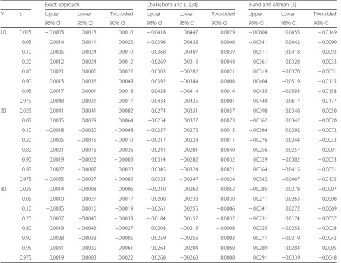
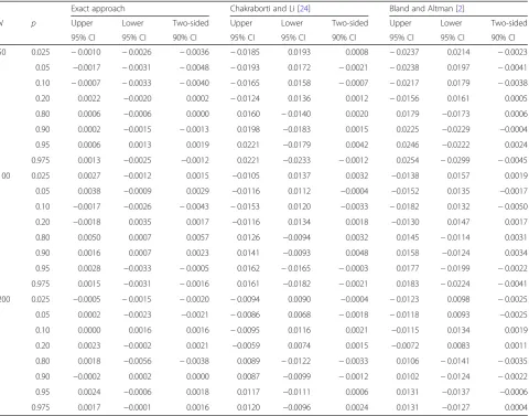
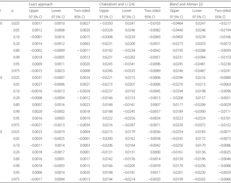
percentile probabilities are examined:p= 0.025, 0.05, 0.10, 0.20, 0.80, 0.90, 0.95, and 0.975. For each replicate, the lower and upper confidence limits {^θL,^θU}, {^θAL,^θAU}, and {^θBAL,θ^BAU} were computed to construct the 95 and 97.5% one-sided confidence intervals and the corresponding 90 and 95% two-sided confidence intervals. The simulated coverage probability was the proportion of the 10,000 rep-licates whose confidence interval contained the population normal percentile. Then, the adequacy of the one- and two-sided interval procedures is determined by the error = simulated coverage probability– nominal coverage prob-ability. The results are summarized in Tables1,2,3and4 for the exact and approximate confidence intervals with two-sided confidence coefficient 1 – α= 0.90 and 0.95, respectively.
Sample size determinations
From a study design viewpoint, it is essential to determine the optimal sample sizes so that the resulting confidence interval will meet the designated precision requirement. Two particularly useful criteria concern the control of the expected width and the assurance probability of the width within a designated bound (Beal [26]; Kupper & Hafner [27]).
The width of the 100(1 – α)% two-sided confidence intervals {^θL,^θU} given in Eq.7is
W¼ t1−α=2 v;zpN1=2
−tα=2 v;zpN1=2
n o
S=N1=2
: ð17Þ
Accordingly, it is desired to calculate the least sam-ple size such that the expected width of a 100(1 – α)
% two-sided confidence interval is within the given threshold:
E W½ ≤δ; ð18Þ
whereδ(> 0) is a constant. On the other hand, one may compute the minimum sample size needed to guarantee, with a given assurance probability, that the width of a 100(1 – α)% two-sided confidence interval will not exceed the planned value:
P Wð ≤ωÞ≥1−γ; ð19Þ
where 1 –γ is the specified assurance level andω (> 0) is a constant.
Under the normal assumption, the assessments of expected width and assurance probability are further simplified for brevity. Note that the expected width E[W] has the alternative form
Table 1The error between simulated coverage probability and nominal coverage probability for the 90% two-sided and 95% one-sided confidence intervals whenN= 10, 20, and 30
Exact approach Chakraborti and Li [24] Bland and Altman [2]
N p Upper Lower Two-sided Upper Lower Two-sided Upper Lower Two-sided 95% CI 95% CI 90% CI 95% CI 95% CI 90% CI 95% CI 95% CI 90% CI
10 0.025 −0.0003 0.0013 0.0010 −0.0418 0.0447 0.0029 −0.0604 0.0455 −0.0149
0.05 0.0014 0.0011 0.0025 −0.0396 0.0436 0.0040 −0.0541 0.0442 −0.0099
0.10 −0.0005 0.0024 0.0019 −0.0368 0.0407 0.0039 −0.0511 0.0418 −0.0093
0.20 0.0012 −0.0024 −0.0012 −0.0269 0.0313 0.0044 −0.0361 0.0328 −0.0033
0.80 0.0021 0.0006 0.0027 0.0303 −0.0282 0.0021 0.0319 −0.0370 −0.0051
0.90 0.0013 0.0036 0.0049 0.0392 −0.0384 0.0008 0.0404 −0.0519 −0.0115
0.95 0.0017 0.0001 0.0018 0.0428 −0.0414 0.0014 0.0435 −0.0593 −0.0158
0.975 −0.0048 0.0031 −0.0017 0.0434 −0.0435 −0.0001 0.0440 −0.0617 −0.0177
20 0.025 0.0041 0.0041 0.0082 −0.0274 0.0331 0.0057 −0.0398 0.0348 −0.0050
0.05 0.0035 0.0029 0.0064 −0.0254 0.0327 0.0073 −0.0362 0.0342 −0.0020
0.10 −0.0018 −0.0030 −0.0048 −0.0257 0.0272 0.0015 −0.0364 0.0292 −0.0072
0.20 0.0005 −0.0015 −0.0010 −0.0217 0.0228 0.0011 −0.0276 0.0244 −0.0032
0.80 0.0021 0.0015 0.0036 0.0241 −0.0201 0.0040 0.0256 −0.0257 −0.0001
0.90 0.0019 −0.0022 −0.0003 0.0314 −0.0282 0.0032 0.0329 −0.0382 −0.0053
0.95 0.0027 −0.0007 0.0020 0.0345 −0.0324 0.0021 0.0364 −0.0415 −0.0051
0.975 −0.0055 −0.0027 −0.0082 0.0323 −0.0347 −0.0024 0.0342 −0.0467 −0.0125
30 0.025 0.0014 −0.0008 0.0006 −0.0210 0.0262 0.0052 −0.0285 0.0278 −0.0007
0.05 0.0010 −0.0027 −0.0017 −0.0208 0.0238 0.0030 −0.0271 0.0263 −0.0008
0.10 −0.0035 0.0016 −0.0019 −0.0261 0.0255 −0.0006 −0.0341 0.0272 −0.0069
0.20 0.0007 −0.0040 −0.0033 −0.0184 0.0152 −0.0032 −0.0231 0.0174 −0.0057
0.80 0.0019 −0.0046 −0.0027 0.0208 −0.0216 −0.0008 0.0225 −0.0253 −0.0028
0.90 0.0028 −0.0033 −0.0005 0.0259 −0.0256 0.0003 0.0277 −0.0319 −0.0042
0.95 0.0031 0.0030 0.0061 0.0264 −0.0204 0.0060 0.0289 −0.0284 0.0005
E W½ ¼ t1−α=2 v;zpN1=2
−tα=2 v;zpN1=2
n o
σ=cN1=2
n o
:
ð20Þ
Hence, the inequality E[W]≤δ is expressed as {t1−α/2(ν, zpN1/2) – tα/2(ν, zpN1/2)}/(cN1/2)≤δ/σ. Also, the assurance probability is equivalent to
P Wð ≤ωÞ ¼P Kð <κÞ ¼Φ κð Þ; ð21Þ
whereK=νS2/σ2~χ2(ν) is a chi-square distribution withν degrees of freedom,κ= {N(N– 1)(ω/σ)2}/{t1−α/2(ν,zpN1/2)
– tα/2(ν, zpN1/2)}2, and Φ(·) is the cumulative distribution
function of the chi-square random variable K. With the exact computational formulas of expected width and assurance probability given in Eqs. 20 and 21, respectively, the sample size N needed to attain the specified precision can be found with a simple itera-tive search for the chosen parameter values {μ, σ2
}, percentile p, and confidence level 1 – α.
Evidently, the sample size determinations do not depend on the mean value μ and reduce to the sample size procedures of Kupper and Hafner [27] becauseθ=μ when p= 0.5. The precision evaluations of expected width and assurance probability depend on the thresholdsδandωthrough the relative magnitude ratios δ/σ and ω/σ, respectively. Accordingly, supplementary SAS/IML and R computer programs are presented to facilitate the required computations. Due to the prospective nature of advance research planning, the general guidelines suggest that typical sources like published findings or expert opinions can offer plausible and reasonable values for the vital characteristics of future study. For illustration, the sample statistics of the blood pressure data in Bland and Altman [2] are adopted as parameter valuesμ=−16.29 andσ= 19.61. Withδ=ω = (0.7)σ= 9.805 and 1 – γ= 0.9, the optimal sample sizes for precise 95% interval estimation of the 97.5th per-centile are 183 and 207 under the expected width Table 2The error between simulated coverage probability and nominal coverage probability for the 90% two-sided and 95% one-sided confidence intervals whenN= 50, 100, and 200
Exact approach Chakraborti and Li [24] Bland and Altman [2]
N p Upper Lower Two-sided Upper Lower Two-sided Upper Lower Two-sided 95% CI 95% CI 90% CI 95% CI 95% CI 90% CI 95% CI 95% CI 90% CI
50 0.025 −0.0010 −0.0026 −0.0036 −0.0185 0.0193 0.0008 −0.0237 0.0214 −0.0023
0.05 −0.0017 −0.0031 −0.0048 −0.0193 0.0172 −0.0021 −0.0238 0.0197 −0.0041
0.10 −0.0007 −0.0033 −0.0040 −0.0165 0.0158 −0.0007 −0.0217 0.0179 −0.0038
0.20 0.0022 −0.0020 0.0002 −0.0124 0.0136 0.0012 −0.0156 0.0161 0.0005
0.80 0.0006 −0.0006 0.0000 0.0160 −0.0140 0.0020 0.0179 −0.0173 0.0006
0.90 0.0002 −0.0015 −0.0013 0.0198 −0.0183 0.0015 0.0225 −0.0229 −0.0004
0.95 0.0006 0.0013 0.0019 0.0221 −0.0179 0.0042 0.0246 −0.0222 0.0024
0.975 0.0013 −0.0025 −0.0012 0.0221 −0.0233 −0.0012 0.0254 −0.0299 −0.0045
100 0.025 0.0027 −0.0012 0.0015 −0.0105 0.0137 0.0032 −0.0138 0.0157 0.0019
0.05 0.0038 −0.0009 0.0029 −0.0116 0.0112 −0.0004 −0.0152 0.0135 −0.0017
0.10 −0.0017 −0.0026 −0.0043 −0.0153 0.0120 −0.0033 −0.0182 0.0132 −0.0050
0.20 −0.0018 0.0035 0.0017 −0.0116 0.0134 0.0018 −0.0130 0.0147 0.0017
0.80 0.0050 0.0007 0.0057 0.0126 −0.0094 0.0032 0.0145 −0.0114 0.0031
0.90 0.0016 0.0007 0.0023 0.0141 −0.0093 0.0048 0.0158 −0.0124 0.0034
0.95 0.0028 −0.0033 −0.0005 0.0162 −0.0165 −0.0003 0.0177 −0.0199 −0.0022
0.975 0.0015 −0.0031 −0.0016 0.0161 −0.0182 −0.0021 0.0183 −0.0224 −0.0041
200 0.025 −0.0005 −0.0015 −0.0020 −0.0094 0.0090 −0.0004 −0.0123 0.0098 −0.0025
0.05 0.0002 −0.0023 −0.0021 −0.0086 0.0068 −0.0018 −0.0118 0.0093 −0.0025
0.10 0.0000 0.0016 0.0016 −0.0095 0.0116 0.0021 −0.0115 0.0134 0.0019
0.20 0.0023 −0.0002 0.0021 −0.0059 0.0074 0.0015 −0.0072 0.0083 0.0011
0.80 0.0018 −0.0056 −0.0038 0.0089 −0.0122 −0.0033 0.0106 −0.0141 −0.0035
0.90 −0.0002 0.0002 0.0000 0.0087 −0.0099 −0.0012 0.0102 −0.0124 −0.0022
0.95 0.0024 −0.0006 0.0018 0.0117 −0.0111 0.0006 0.0131 −0.0137 −0.0006
and assurance probability criteria, respectively. For ease of application, the prescribed configurations are incorporated in the user specification sections of the SAS/IML (Additional files 1, 2 and 3) and R programs (Additional files 4, 5 and 6).
To further demonstrate the features and differences of the two suggested sample size procedures for precise interval estimation of the normal percentiles, numerical computations are performed forp= 0.025, 0.05, 0.10, 0.20, 0.30, 0.40, 0.50, 0.60, 0.70, 0.80, 0.90, 0.95, and 0.975 under the expected width and assurance probability criteria. The parameter configurations are fixed asμ= 0,σ2= 1, 1–α= 0.95 throughout the empirical appraisal. Moreover, the selected two thresholds of expected width are δ= 0.5 and 1.0. For assurance evaluation, the four designated settings are 1 – γ= 0.80 and 0.9 combined withω= 0.5 and 1.0. These configurations are chosen to reflect common sample sizes used in typical research settings.
For ease of illustration, the computed sample sizes are plotted in Fig.2.
It is seen from Fig.2for the six types of precision that the graphs of the optimal sample size are symmetric with respect to p= 0.5 and are monotonously increasing with the absolute difference |p – 0.5|. Therefore, the required sample size for precise interval estimation of median or mean is smaller than those of the other nor-mal percentiles. Also, the optinor-mal sample size increases with a smaller width bound of δ and ω when all other factors are fixed. As expected, more sample size is needed to attain a higher assurance level 1–γwhen the designated width ω and other configurations remain identical. Regarding the difference between the two pre-cision principles, it typically requires a larger sample size to meet the necessary precision of assurance probability than the control of a designated expected width. With the same interval bound δ=ω, the sample sizes Table 3The error between simulated coverage probability and nominal coverage probability for the 95% two-sided and 97.5% one-sided whenN= 10, 20, and 30
Exact approach Chakraborti and Li [24] Bland and Altman [2]
N p Upper Lower Two-sided Upper Lower Two-sided Upper Lower Two-sided 97.5% CI 97.5% CI 95% CI 97.5% CI 97.5% CI 95% CI 97.5% CI 97.5% CI 95% CI
10 0.025 0.0017 0.0010 0.0027 −0.0350 0.0247 −0.0103 −0.0464 0.0247 −0.0217
0.05 0.0012 0.0008 0.0020 −0.0328 0.0246 −0.0082 −0.0440 0.0246 −0.0194
0.10 −0.0001 0.0016 0.0015 −0.0308 0.0239 −0.0069 −0.0405 0.0239 −0.0166
0.20 0.0014 −0.0012 0.0002 −0.0231 0.0200 −0.0031 −0.0275 0.0203 −0.0072
0.80 −0.0002 −0.0009 −0.0011 0.0192 −0.0234 −0.0042 0.0195 −0.0288 −0.0093
0.90 0.0018 −0.0005 0.0013 0.0231 −0.0282 −0.0051 0.0231 −0.0384 −0.0153
0.95 0.0009 0.0011 0.0020 0.0245 −0.0341 −0.0096 0.0245 −0.0481 −0.0236
0.975 −0.0015 0.0023 0.0008 0.0246 −0.0335 −0.0089 0.0246 −0.0487 −0.0241
20 0.025 0.0031 −0.0007 0.0024 −0.0221 0.0215 −0.0006 −0.0296 0.0216 −0.0080
0.05 0.0027 −0.0006 0.0021 −0.0213 0.0207 −0.0006 −0.0276 0.0213 −0.0063
0.10 −0.0016 −0.0013 −0.0029 −0.0237 0.0192 −0.0045 −0.0294 0.0198 −0.0096
0.20 −0.0008 −0.0004 −0.0012 −0.0166 0.0153 −0.0013 −0.0208 0.0157 −0.0051
0.80 0.0007 0.0016 0.0023 0.0168 −0.0161 0.0007 0.0177 −0.0206 −0.0029
0.90 0.0020 −0.0002 0.0018 0.0188 −0.0245 −0.0057 0.0189 −0.0300 −0.0111
0.95 0.0016 0.0003 0.0019 0.0222 −0.0256 −0.0034 0.0223 −0.0324 −0.0101
0.975 −0.0021 −0.0013 −0.0034 0.0216 −0.0287 −0.0071 0.0220 −0.0372 −0.0152
30 0.025 0.0023 −0.0019 0.0004 −0.0215 0.0179 −0.0036 −0.0254 0.0183 −0.0071
0.05 0.0024 −0.0025 −0.0001 −0.0200 0.0162 −0.0038 −0.0245 0.0172 −0.0073
0.10 −0.0011 0.0014 0.0003 −0.0206 0.0164 −0.0042 −0.0256 0.0170 −0.0086
0.20 0.0018 −0.0017 0.0001 −0.0131 0.0131 0.0000 −0.0161 0.0136 −0.0025
0.80 0.0016 0.0001 0.0017 0.0142 −0.0156 −0.0014 0.0150 −0.0196 −0.0046
0.90 0.0018 −0.0003 0.0015 0.0166 −0.0205 −0.0039 0.0170 −0.0256 −0.0086
0.95 0.0006 0.0014 0.0020 0.0198 −0.0181 0.0017 0.0201 −0.0230 −0.0029
associated with the assurance criterion are larger than those under the expected width consideration. For the precision settings considered here, the sample sizes for δ/σ=ω/σ= 1.0 are within the range of [40, 60] forp= 0.95 and 0.975. With δ/σ=ω/σ= 0.5, the computed sample sizes for the same percentiles are much larger and have a wider interval [148, 207]. These numerical illustrations suggest that the width boundsδ/σ=ω/σ= 0.5 and 1.0 and the assurance level 1–γ= 0.80 and 0.90 lead to sensible sample sizes and are suitable benchmark precision setups for designing percentile studies. Deciding on the appropri-ate precision requirements always requires careful thought and should be determined by the research context and study goal within a particular scientific field.
Discussion
In view of the wide application in medical studies, this article aims to explicate the theoretical and empirical features of interval procedures of percentiles. An
integrated discussion is presented to address the similar-ities and differences of exact and approximate confi-dence intervals constructed with various pivotal quantities described in the literature. Although there are distinct selections of pivotal quantities, it is shown that they yield the same exact confidence intervals. Notably, the exact interval procedure requires the use of the cumulative distribution function of a noncentralt distri-bution. The difficulty of applying the exact approach has been alleviated because of the availability of specialized routines in popular software packages. In contrast, the approximate interval methods are computationally simple and do not require specialized software because they only involve the quantiles of a regulartdistribution. However, the approximate confidence intervals carry the symmetry property of a t distribution whereas the noncentral tdistribution is skewed so that the resulting exact confidence intervals are not equidistant around the primary statistic.
Table 4The error between simulated coverage probability and nominal coverage probability for the 95% two-sided and 97.5% one-sided confidence intervals whenN= 50, 100, and 200
Exact approach Chakraborti and Li [24] Bland and Altman [2]
N p Upper Lower Two-sided Upper Lower Two-sided Upper Lower Two-sided 97.5% CI 97.5% CI 95% CI 97.5% CI 97.5% CI 95% CI 97.5% CI 97.5% CI 95% CI
50 0.025 −0.0004 −0.0022 −0.0026 −0.0188 0.0144 −0.0044 −0.0221 0.0157 −0.0064
0.05 −0.0002 −0.0026 −0.0028 −0.0169 0.0131 −0.0038 −0.0208 0.0145 −0.0063
0.10 0.0007 −0.0018 −0.0011 −0.0135 0.0104 −0.0031 −0.0164 0.0120 −0.0044
0.20 0.0009 −0.0020 −0.0011 −0.0083 0.0084 0.0001 −0.0105 0.0089 −0.0016
0.80 −0.0001 −0.0008 −0.0009 0.0102 −0.0114 −0.0012 0.0112 −0.0132 −0.0020
0.90 0.0020 −0.0017 0.0003 0.0138 −0.0161 −0.0023 0.0146 −0.0189 −0.0043
0.95 0.0031 0.0006 0.0037 0.0159 −0.0145 0.0014 0.0161 −0.0183 −0.0022
0.975 0.0014 −0.0010 0.0004 0.0160 −0.0182 −0.0022 0.0167 −0.0227 −0.0060
100 0.025 0.0015 −0.0017 −0.0002 −0.0096 0.0105 0.0009 −0.0119 0.0116 −0.0003
0.05 0.0007 −0.0030 −0.0023 −0.0090 0.0091 0.0001 −0.0108 0.0106 −0.0002
0.10 0.0002 −0.0008 −0.0006 −0.0106 0.0095 −0.0011 −0.0128 0.0101 −0.0027
0.20 −0.0002 0.0035 0.0033 −0.0090 0.0110 0.0020 −0.0104 0.0115 0.0011
0.80 0.0014 0.0008 0.0022 0.0088 −0.0075 0.0013 0.0092 −0.0094 −0.0002
0.90 0.0005 0.0000 0.0005 0.0111 −0.0096 0.0015 0.0121 −0.0120 0.0001
0.95 0.0013 −0.0012 0.0001 0.0115 −0.0143 −0.0028 0.0117 −0.0164 −0.0047
0.975 0.0014 −0.0011 0.0003 0.0118 −0.0140 −0.0022 0.0125 −0.0160 −0.0035
200 0.025 0.0006 −0.0019 −0.0013 −0.0066 0.0077 0.0011 −0.0084 0.0084 0.0000
0.05 0.0021 −0.0013 0.0008 −0.0056 0.0075 0.0019 −0.0077 0.0079 0.0002
0.10 0.0005 0.0023 0.0028 −0.0068 0.0088 0.0020 −0.0079 0.0095 0.0016
0.20 0.0012 −0.0012 0.0000 −0.0042 0.0047 0.0005 −0.0052 0.0053 0.0001
0.80 0.0029 −0.0017 0.0012 0.0077 −0.0077 0.0000 0.0080 −0.0095 −0.0015
0.90 −0.0015 −0.0001 −0.0016 0.0054 −0.0070 −0.0016 0.0061 −0.0085 −0.0024
0.95 0.0020 −0.0021 −0.0001 0.0100 −0.0089 0.0011 0.0104 −0.0100 0.0004
Fig. 1Coverage probability of 97.5% one-sided confidence interval forN= 10
Conclusions
Despite the positive findings in previous research, detailed numerical assessments are presented to reveal the under-lying drawbacks of the approximate methods under the notion that the endpoints of a two-sided confidence interval have a corresponding interpretation as a lower or upper confidence limit of a one-sided confidence interval. Essen-tially, the simplicity and symmetry of an approximate confi-dence interval generally do not maintain the assumption of equal-tailed error rates for the two individual endpoints. For the purpose of planning percentile studies so that the results will help confirm meaningful reference targets, sample size procedures for precise interval estimation of normal percentiles are described under the precision criteria of expected width and assurance probability. To enhance the applicability of the exact interval approach and corresponding sample size methodologies, computer codes are also presented to perform the required computations.
Additional files
Additional file 1:SAS/IML program for computing the exact confidence interval of percentile. (DOCX 64 kb)
Additional file 2:SAS/IML program for computing sample size required to meet the designated expected width for confidence interval of percentile. (DOCX 64 kb)
Additional file 3:SAS/IML program for computing sample size required to ensure adequate assurance probability of achieving the desired width for confidence interval of percentile. (DOCX 67 kb)
Additional file 4:R program for computing the exact confidence interval of percentile. (DOCX 62 kb)
Additional file 5:R program for computing sample size required to meet the designated expected width for confidence interval of percentile. (DOCX 64 kb)
Additional file 6:R program for computing sample size required to ensure adequate assurance probability of achieving the desired width for confidence interval of percentile. (DOCX 20 kb)
Funding
This work was supported by a grant from the Ministry of Science and Technology of Taiwan (MOST 105–2410-H-009-035-MY2). The fund supported the author to design the study, conduct statistical analysis, and write the manuscript.
Availability of data and materials
The summary statistics are available from the following article: [2].
Author’s contributions
GS conceived of the study, conducted the theoretical examination, carried out the numerical computations, and drafted the manuscript. The author read and approved the final manuscript.
Ethics approval and consent to participate
Not applicable.
Competing interests
The author declares that she has no competing interests.
Publisher’s Note
Springer Nature remains neutral with regard to jurisdictional claims in published maps and institutional affiliations.
Received: 14 July 2017 Accepted: 3 May 2018
References
1. Bland JM, Altman D. Statistical methods for assessing agreement between two methods of clinical measurement. Lancet. 1986;327:307–10.
2. Bland JM, Altman DG. Measuring agreement in method comparison studies. Stat Methods Med Res. 1999;8:135–60.
3. Royston P, Matthews JNS. Estimation of reference ranges from normal samples. Stat Med. 1991;10:691–5.
4. Keating JP, Mason RL, Balakrishnan N. Percentile estimators in location-scale parameter families under absolute loss. Metrika. 2010;72:351–67.
5. Keating JP, Tripathi RC. Percentiles, estimation of, encyclopedia of statistical sciences, vol. VI. New York: Wiley; 1985. p. 668–74.
6. Parrish RS. Comparison of quantile estimators in normal sampling. Biometrics. 1990;46:247–57.
7. Rukhin AL. A class of minimax estimators of a normal quantile. Stat Probabil Lett. 1983;1:217–21.
8. Zidek JV. Inadmissibility of the best invariant estimator of extreme quantiles of the normal law under squared error loss. Ann Math Stat. 1969;40:1801–8. 9. Zidek JV. Inadmissibility of a class of estimators of a normal quantile. Ann
Math Stat. 1971;42:1444.
10. Hahn GJ. Statistical intervals for a normal population, part I. Tables, examples and applications. J Qual Technol. 1970;2:115–25.
11. Hahn GJ. Statistical intervals for a normal population, part II. Formulas, assumptions, some derivations. J Qual Technol. 1970;2:195–206. 12. Hahn GJ, Meeker WQ. Statistical intervals: a guide for practitioners. New
York: Wiley; 1991.
13. Vardeman SB. What about the other intervals? Am Stat. 1992;46:193–7. 14. Johnson NL, Kotz S, Balakrishnan N. Continuous univariate distributions, vol.
2. 2nd ed. New York: Wiley; 1995.
15. Owen DB. A survey of properties and applications of the noncentral t-distribution. Technometrics. 1968;10:445–78.
16. David HA, Nagaraja HN. Order statistics. 3rd ed. New York: Wiley; 2003. 17. Krishnamoorthy K, Mathew T. Statistical tolerance regions: theory,
applications, and computation, vol. 744. New York: Wiley; 2009.
18. Odeh RE, Owen DB. Tables for normal tolerance limits, sampling plans, and screening. New York: Marcel Dekker; 1980.
19. Carkeet A. Exact parametric confidence intervals for Bland-Altman limits of agreement. Optom Vis Sci. 2015;92:e71–80.
20. Carkeet A, Goh YT. Confidence and coverage for Bland-Altman limits of agreement and their approximate confidence intervals. Stat Methods Med Res. 2018;27:1559–74.
21. Barnhart HX, Haber MJ, Lin LI. An overview on assessing agreement with continuous measurements. J Biopharm Stat. 2007;17:529–69.
22. Choudhary PK, Nagaraja HN. Measuring agreement in method comparison studies–a review. In: Balakrishnan N, Kannan N, Nagaraja HN, editors. Advances in ranking and selection, multiple comparisons, and reliability. Boston: Birkhauser; 2004. p. 215–44.
23. Lin LI, Hedayat AS, Sinha B, et al. Statistical methods in assessing agreement: models, issues and tools. J Am Stat Assoc. 2002;97:257–70. 24. Chakraborti S, Li J. Confidence interval estimation of a normal percentile.
Am Stat. 2007;61:331–6.
25. Lawless JF. Statistical models and methods for lifetime data. 2nd ed. New York: Wiley; 2003.
26. Beal SL. Sample size determination for confidence intervals on the population mean and on the difference between two population means. Biometrics. 1989;45:969–77.