Interim analyses of data as they accumulate in laboratory experimentation

Open Access

Debate

Interim analyses of data as they accumulate in laboratory

experimentation

John Ludbrook*

Address: Department of Surgery, The University of Melbourne, Parkville, Victoria, Australia (563 Canning Street, Carlton North, Victoria 3054, Australia)

Email: John Ludbrook* - [email protected] * Corresponding author

Abstract

Background: Techniques for interim analysis, the statistical analysis of results while they are still accumulating, are highly-developed in the setting of clinical trials. But in the setting of laboratory experiments such analyses are usually conducted secretly and with no provisions for the necessary adjustments of the Type I error-rate.

Discussion: Laboratory researchers, from ignorance or by design, often analyse their results before the final number of experimental units (humans, animals, tissues or cells) has been reached. If this is done in an uncontrolled fashion, the pejorative term 'peeking' has been applied. A statistical penalty must be exacted. This is because if enough interim analyses are conducted, and if the outcome of the trial is on the borderline between 'significant' and 'not significant', ultimately one of the analyses will result in the magical P = 0.05. I suggest that Armitage's technique of matched-pairs sequential analysis should be considered. The conditions for using this technique are ideal: almost unlimited opportunity for matched pairing, and a short time between commencement of a study and its completion. Both the Type I and Type II error-rates are controlled. And the maximum number of pairs necessary to achieve an outcome, whether P = 0.05 or P > 0.05, can be estimated in advance.

Summary: Laboratory investigators, if they are to be honest, must adjust the critical value of P if they analyse their data repeatedly. I suggest they should consider employing matched-pairs sequential analysis in designing their experiments.

Background

What does the term 'interim analysis' mean? A short defi-nition is that it refers to the repeated analyses of data as they accumulate. This is not a bad definition, since it can be applied not only to clinical trials but also to laboratory experiments.

Why does it matter? It matters in a statistical sense that is

of Type I error (false-positive inference) increases progres-sively as the number of tests of significance increases. I have reviewed elsewhere the problem of making multiple comparisons and ways of solving it [1,2]. Here I review the topic of making serial comparisons on data as they accu-mulate. To state this problem in a very crude, but none-theless broadly accurate, fashion it is almost inevitable that if the outcome is on the borderline of significance,

≤ Published: 21 August 2003

BMC Medical Research Methodology 2003, 3:15

Received: 23 April 2003 Accepted: 21 August 2003

This article is available from: http://www.biomedcentral.com/1471-2288/3/15

In the context of clinical trials, the issue of interim analy-sis is not a new one. It has been discussed in the statistical literature since the 1960s, and has reached the level of consciousness of clinical trialists over the last few years. For instance, the number of 'hits' in a PubMed search (National Library of Medicine, Washington DC) that I conducted for (interim AND analysis) were: 1968–70 (0), 1978–80 (10), 1988–90 (67), 1998–2000 (214). In 2001–2003 there were 252 hits. In the earlier periods, papers dealt chiefly with theoretical issues. In the later periods, most were concerned with actual clinical trials.

Discussion

Clinical trials

Several statistical techniques for dealing with interim analyses of clinical trials have been described. These include, in order of appearance, the Armitage-McPherson [3], Pocock [4,5], Haybittle-Peto [6,7] and O'Brien-Flem-ing [8] methods. All these techniques depend on the interim analyses being planned in advance. Excellent, simple descriptions of these can be found in the book by Friedman et al. [9]. A simulation study suggests that the O'Brien-Fleming technique is the most powerful of these [10]. Lan & DeMets introduced the notion of the adaptive,

α-spending, function, that could be applied to unplanned interim analyses [11,12]. However, this has been severely criticised by theoretical statisticians [13]. Then there is the Bayesian approach, well-described by Jennison & Turn-bull [14], but rarely employed.

Laboratory experiments

None of the techniques for interim analysis of clinical tri-als is applicable, or easily adaptable, to the unplanned sta-tistical analyses of laboratory experiments, usually undertaken covertly rather than overtly.

There are good reasons and bad reasons for performing interim analyses of laboratory experiments.

A good reason is that the investigators have made, in advance, an estimate of minimal group (sample) size. But they are not confident that it is a good estimate. This may be, for instance, because they have had to base their

esti-mate on others' published data or because it is based on a small set of pilot experiments. It is reasonable, therefore, that they should analyze the results when their estimated minimal group size has been attained. If their null hypothesis is rejected, they can stop. If not, they can then use these results to re-estimate minimal group size and carry on.

A bad reason is that the investigators have not formally estimated minimal group size, but have merely made a guess. They carry out the first round of experiments, test the results, and find that they are not quite 'significant'. So they do a few more experiments. Still not quite there. So they do a few more experiments – and so on until they achieve P = 0.05, or give up.

What solutions are there to this problem? One is to employ relatively simple methods for adjusting the critical value of P. An altogether different approach is to use a technique called matched-pairs sequential analysis. A third approach, already hinted at, is to re-estimate mini-mal group size.

Simple methods for adjusting the critical value of P

The Šidák inequality [15] plays an important role in mul-tiple comparison procedures [1,2]. This means that the adjusted critical value of P is given by the formula 1 (1

-P)k_{, where k is the number of interim analyses and the} nominal critical value of P is usually 0.05. Alternatively, the raw P value resulting from a test of significance can be adjusted by the formula P' = 1 - (1 - P)1/k_.

The Šidák adjustment is a severe one (Table 1). Why is this? It is appropriate for multiple comparisons when these are completely independent. But it is obvious that successive interim analyses are not independent of each other, but to some degree correlated. This is also true of many (most) sets of multiple comparisons [2]. For this reason the Šidák adjustment is unsuited to planned interim analyses. However, it may have a place for the sin-gle, unplanned, interim analysis when, to put it bluntly, the investigators should pay a high penalty.

Table 1: The results of applying the Šidák [15] and Armitage-McPherson [3] adjustments

No. of interim analyses (k) Nominal critical

P value

Adjusted critical P value

(Šidák) (Armitage-McPherson)

1 0.05 0.050 0.050

2 0.05 0.025 0.030

5 0.05 0.010 0.016

10 0.05 0.005 0.011

The Armitage-McPherson adjustment [16,17] is a little less severe than the Šidák adjustment (Table 1), but has the same drawback that independence of the interim anal-yses is assumed.

Matched-pairs sequential analysis

This technique is attributed to Wald [18]. He was able to publish it only after World War II because during the war it had been classified as an economical and sensitive tech-nique for testing munitions. Armitage suggested it as a

technique for use in clinical trials [19,20]. However, it has been used infrequently in this connection, for reasons given below. Kilpatrick & Oldham were the first to use the technique in an actual clinical trial [21], though in a rather crude, one-sided, fashion. An interesting example of its use is in a clinical trial of the therapeutic efficacy of prayer [22]. My own experience with it is confined to a trial of the efficacy of rose-preserving solutions (see Fig. 1) [23].

An example of matched-pairs sequential analysis [23]

Figure 1

An example of matched-pairs sequential analysis [23]. The experiment was designed to test the relative efficacy of: (A) a solu-tion of inorganic chemicals dissolved in rainwater (Kaltaler solusolu-tion); and (B) rainwater (tankwater), on the vase-life of roses. The end-point was time to first petal-fall. The graphical design relied on 2α = 0.05 or 0.01, 1 - β (power) = 0.95. θ was set at 0.90. Left panel: 2α set at 0.05. Kaltaler solution was superior to rainwater because the upper boundary was crossed at N =

11. A preference for B occurred only at preference number 5. Right panel: 2α set at 0.01. There was no significant difference

because the right boundary was crossed at N = 23. A preference for B occurred only at preference numbers 5, 12, 17, 18 and 23. Confirmatory post hoc exact, two-sided, tests of the null hypothesis that for a single binomial p = 0.50 gave P = 0.012 for the left-hand panel (ie. P = 0.05), and P = 0.011 (ie. P > 0.01) for the right-hand panel (StatXact 5, Cytel Software Corporation, Cambridge MA).

5

10

15

5

10

15

2

α

= 0.05

2

α

= 0.01

Preference

for A

Preference

for A

Preference

for B

Preference

_{for B}

0

0

No Preference

No Preference

A simplified description of the technique is as follows. Matched pairs of subjects are assembled, and the mem-bers of each pair are assigned randomly to one or the other treatment to be investigated. The analysis is graphi-cal. Horizontal, V-shaped, statistically-defined, upper and lower boundaries are constructed. The outcome of the trial for each pair is scored as a preference for treatment A or treatment B, and entered into the graph. If the zigzag line described by successive pairs crosses one or the other boundary, it can safely be concluded that A is superior to B (or vice versa) at a specified nominal level of significance (for instance, two-sided P = 0.05). In the preferred closed, or restricted, design a third boundary is placed across the open end of the V. If this is crossed first, then at a specified Type II error-rate it can be concluded that there is no sig-nificant difference between the treatments [20]. The advantage of this approach is that both the Type I and Type II error-rates are controlled, and the maximum number of matched pairs necessary to cross one or another boundary can be predicted. The coordinates of the graphical boundaries are determined by: (a) the selected two-sided Type I error-rate (2α = 0.05, 0.01); (b) the selected Type II error-rate, β, where (1 - β) = power to reject the null hypothesis; and (c) the θ statistic. Typical values of these are 2α = 0.05 or 0.01, β = 0.05, θ = 0.90 (see Fig. 1).

The strength of the matched-pairs technique is that it ensures that an inference will be reached (A>B, B>A or A = B) with a predictable maximum number of paired sub-jects. However, it has serious practical limitations that have greatly restricted its use in clinical trials. These are that: (a) there must be a large reservoir of eligible patients so that matching can be done; (b) the time from entry to outcome must be short compared with the expected dura-tion of the trial; and (c) the technique cannot be applied to tests on survival curves such as the logrank (Mantel-Haenszel) test. For these reasons, group sequential

analy-sis has been the technique preferred for clinical trials [24– 26].

If even amateur biostatisticians follow the instructions given by Armitage [19,20], they should be able to design the graphical boundaries for a closed (restricted) matched-pairs sequential analysis. If they (or reviewers) have doubts about the outcome, they can use an exact test on a single binomial to confirm the inferences (see Fig. 1).

I have been unable to find an example of its use in labo-ratory experiments, with the exception of my obscurely-published trial of rose preservatives [23]. Yet there is an almost unlimited supply of laboratory animals that can be matched for characteristics such as sex, age and weight. The outcome of the experiment is usually available within hours, days or weeks. The only reservation is that if the outcome of the experiment is measured on a continuous scale, there may be some loss of power because for the purpose of graphical analysis the outcomes are converted into a binomial preference for one treatment over another.

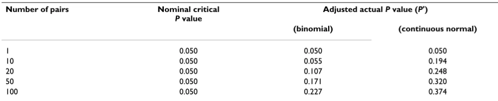
Later, Armitage and colleagues [16], and McPherson & Armitage [3] addressed the matter from a somewhat dif-ferent perspective and by difdif-ferent statistical techniques. They called this 'repeated significance testing' (RST). The requirement of matched-pairs remained, but they calcu-lated (or obtained by simulation) the actual significance levels corresponding to nominal levels for serial repeated testing, for both binomial and continuous (normally-dis-tributed) outcomes. This results in parabolic boundaries, rather than the linear boundaries of Fig. 1[3]. If N (the number of matched-pairs) is greater than 10–15, the par-abolic and linear boundaries are very similar. An example of their work is in Table 2 and Figure 2. If the outcome measure is normally-distributed, the RST approach is to be preferred. If investigators consider using this, it is best that they consult an experienced biostatistician.

Table 2: Adjusted P values corresponding to a raw P = 0.05 for binomial and continuous outcomes, according to the number of matched-pairs tested. After Armitage et al. [16]

Number of pairs Nominal critical

P value

Adjusted actual P value (P')

(binomial) (continuous normal)

1 0.050 0.050 0.050

10 0.050 0.055 0.194

20 0.050 0.107 0.248

50 0.050 0.171 0.320

Armitage gave an easily-understood account of the matched-pairs technique in 1975 [20]. His book is out of print, but is available in libraries. Alternatively, biomedi-cal investigators and biostatisticians can consult the origi-nal accounts [3,16,19], or Whitehead's book [24].

A third approach

In planning a prospective clinical trial, it is mandatory that minimal group sizes are estimated before the trial starts. This is insisted on by institutional human ethics committees.

Institutional animal ethics committees, at any rate in Aus-tralia, now also insist that minimal group sizes are esti-mated in advance. This can be done on the basis of earlier studies in the same laboratory or, second best, studies published by others. The convention is to make the esti-mate on the basis that the critical value of P is 0.05 at a power of 0.80 (80%). Very useful aids to making these estimates are published tables [27], or interactive compu-ter programs (for instance, nQuery Advisor, Statistical Solutions, Boston MA).

But minimal group size estimates are only as accurate as the data on which they are based. Often these data are sus-pect, or the dataset is too small. So when investigators have done the necessary number of experiments, analysed the results, and find that P is just a little greater than 0.05, it is not unreasonable that they should re-estimate

mini-new estimate exceeds their original one, it is not unrea-sonable that they should carry out further experiments so that the revised estimate is achieved. Then, it is argued, their new and definitive analysis needs no adjustment of the P value.

Summary

There has been a twofold purpose to this review. One has been to remind clinical investigators of the rules govern-ing the interim analysis of results as they accumulate in clinical trials. These rules are very firmly established, thanks to the work of biostatisticians and of regulatory bodies. The second, and more original, reason is to acquaint biologists who are conducting laboratory exper-iments with the price they should pay for analyzing their results as they accumulate, usually to decide whether they need to do more experiments to 'achieve' a magical P = 0.05. Whenever I chastise experimentalists for conducting interim analyses and suggest that they are acting unstatis-tically, if not unethically, they react with surprise.

I hope that this review may bring experimentalists and clinical trialists closer together in their attitudes towards the interim analysis of accumulating results. I believe that laboratory experimenters have a good deal to learn from clinical trialists. In particular, I commend to them matched-pairs sequential analysis as a technique for designing and analyzing their experiments.

Author Contributions

The author was responsible for all aspects of this paper.

Competing Interests

None declared.

Acknowledgements

I am most grateful for the critical comments and suggestions on earlier ver-sions of the manuscript from epidemiologists and laboratory biomedical sci-entists, and from the two reviewers. I do not name them for fear that it might be thought that they approved. Blackwell Publications gave permis-sion for me to reproduce Figure 5.3 from Armitage [20] as Figure 2.

References

1. Ludbrook J: Repeated measurements and multiple compari-sons in cardiovascular research. Cardiovasc Res 1994, 28:303-311. 2. Ludbrook J: Multiple comparison procedures updated. Clin Exp

Pharmacol Physiol 1998, 25:1032-1037.

3. McPherson CK and Armitage P: Repeated significance tests on accumulating data when the null hypothesis is not true. J R Stat Soc A 1971, 134:15-25.

4. Pocock SJ: Group sequential methods in the design and analy-sis of clinical trials. Biometrika 1977, 64:191-199.

5. Pocock SJ: Interim analyses for randomized clinical trials: the group sequential approach. Biometrics 1982, 38:153-162. 6. Haybittle JL: Repeated assessment of results in clinical trials of

cancer treatment. Br J Radiol 1971, 44:793-797.

7. Peto R, Pike MC, Armitage P, Breslow NE, Cox DR, Howard SV, Man-tel N, McPherson K, Peto J and Smith PG: Design and analysis of randomized clinical trials requiring prolonged observation of Redrawn from Fig. 5.3 of Armitage [20], with the kind

per-mission of Blackwell Publishing

Figure 2

Redrawn from Fig. 5.3 of Armitage [20], with the kind per-mission of Blackwell Publishing. 2α = 0.05. β = 0.05. d = dif-ference between means for each matched-pair. γ =

cumulative sum of differences between means. σ = common standard deviation. N = number of matched pairs. _____ = restricted plan. - - - = RST plan.

10 10

-10 20

-20 30

-30

20 30 0

40 50 60 70 80 N

Publish with BioMed Central and every scientist can read your work free of charge

"BioMed Central will be the most significant development for disseminating the results of biomedical researc h in our lifetime."

Sir Paul Nurse, Cancer Research UK

Your research papers will be:

available free of charge to the entire biomedical community

peer reviewed and published immediately upon acceptance

cited in PubMed and archived on PubMed Central

yours — you keep the copyright

Submit your manuscript here:

http://www.biomedcentral.com/info/publishing_adv.asp

BioMedcentral 8. O'Brien PC and Fleming TR: A multiple testing procedure for

clinical trials. Biometrics 1979, 35:549-556.

9. Friedman LM, Furberg CD and DeMets DL: Fundamentals of Clin-ical Trials. St Louis, Mosby 31996.

10. Skovlund E: Repeated significance tests on accumulating data.

J Clin Epidemiol 1999, 52:1083-1088.

11. Lan KKG and DeMets DJ: Discrete sequential boundaries for clinical trials. Biometrika 1983, 70:659-663.

12. Lan KKG and DeMets DL: Changing frequency of interim anal-ysis in sequential monitoring. Biometrics 1989, 45:1017-1020. 13. Tsiatis AA and Mehta C: On the inefficiency of the adaptive

design for monitoring clinical trials. Biometrika 2003, 90:367-378.

14. Jennison C and Turnbull BW: Statistical approaches to interim monitoring of medical trials: a review and commentary. Sta-tistical Science 1990, 5:299-317.

15. Šidák Z: Rectangular confidence regions for the means of mul-tivariate normal distributions. J Am Statist Assoc 1967, 62:626-633.

16. Armitage P, McPherson CK and Rowe BC: Repeated significance tests on accumulating data. J R Stat Soc A 1969, 132:235-244. 17. McPherson K: Statistics: the problem of examining

accumulat-ing data more than once. N Engl J Med 1974, 290:501-502. 18. Wald A: Sequential Analysis. New York, John Wiley & Sons 1947. 19. Armitage P: Sequential tests in prophylactic and therapeutic

trials. Q J Med 1954, 23:255-274.

20. Armitage P: Sequential Medical Trials. Oxford, Blackwell Scientific Publications 21975.

21. Kilpatrick GS and Oldham PD: Calcium chloride and adrenaline as bronchial dilators compared by sequential analysis. Br Med J 1954, ii:1388-1399.

22. Joyce CRB and Welldon RMC: The objective efficacy of prayer: a double-blind clinical trial. J Chron Dis 1965, 18:367-377. 23. Campbell AG, Campbell IAO and Ludbrook J: Lengthening the

vase life of roses. In: The Australian Rose, The National Rose Society of Australia 1975:40-45.

24. Whitehead J: The Design and Analysis of Sequential Clinical Trials. New York, John Wiley & Sons 21997.

25. Chow S-C and Liu J-P: Design and Analysis of Clinical Trials: Concepts and Methodologies. New York, John Wiley & Sons 1998. 26. Jennison C and Turnbull BW: Group Sequential Methods with Applications to Clinical Trials. Boca Raton, Chapman & Hall/CRC

2000.

27. Machin D, Campbell MJ, Fayers PM and Pinol ABY: Sample Size Tables for Clinical Studies. Oxford, Blackwell Science 21997.

Pre-publication history

The pre-publication history for this paper can be accessed here: