R E S E A R C H A R T I C L E
Open Access
Low income, community poverty and risk of end
stage renal disease
Deidra C Crews
1,2*, Orlando M Gutiérrez
3,4, Stacey A Fedewa
5, Jean-Christophe Luthi
5,6, David Shoham
7,
Suzanne E Judd
8, Neil R Powe
9,10and William M McClellan
5,11Abstract
Background:The risk of end stage renal disease (ESRD) is increased among individuals with low income and in low income communities. However, few studies have examined the relation of both individual and community socioeconomic status (SES) with incident ESRD.
Methods:Among 23,314 U.S. adults in the population-based Reasons for Geographic and Racial Differences in Stroke study, we assessed participant differences across geospatially-linked categories of county poverty [outlier poverty, extremely high poverty, very high poverty, high poverty, neither (reference), high affluence and outlier affluence]. Multivariable Cox proportional hazards models were used to examine associations of annual household income and geospatially-linked county poverty measures with incident ESRD, while accounting for death as a competing event using the Fine and Gray method.
Results:There were 158 ESRD cases during follow-up. Incident ESRD rates were 178.8 per 100,000 person-years (105py) in high poverty outlier counties and were 76.3 /105py in affluent outlier counties, p trend = 0.06. In unadjusted competing risk models, persons residing in high poverty outlier counties had higher incidence of ESRD (which was not statistically significant) when compared to those persons residing in counties with neither high poverty nor affluence [hazard ratio (HR) 1.54, 95% Confidence Interval (CI) 0.75-3.20]. This association was markedly attenuated following adjustment for socio-demographic factors (age, sex, race, education, and income); HR 0.96, 95% CI 0.46-2.00. However, in the same adjusted model, income was independently associated with risk of ESRD [HR 3.75, 95% CI 1.62-8.64, comparing the < $20,000 income group to the > $75,000 group]. There were no statistically significant associations of county measures of poverty with incident ESRD, and no evidence of effect modification.
Conclusions:In contrast to annual family income, geospatially-linked measures of county poverty have little relation with risk of ESRD. Efforts to mitigate socioeconomic disparities in kidney disease may be best appropriated at the individual level.
Keywords:ESRD, Chronic kidney disease, Socioeconomic status, Disparity, Geospatial
Background
The risk of end-stage renal disease (ESRD) is increased among low income individuals and in low income com-munities [1]. Low income or poverty status is one of the most frequently studied indicators of low socioeconomic status (SES) at the individual level [2]. Poverty has been associated with multiple risk factors for kidney disease
including hypertension [3], diabetes [4], and obesity [5]; and multiple studies have documented an association of poverty with kidney disease [6-10].
Community measures of SES have also been examined in relation to kidney disease. Volkovaet al.reported that residence in poor U.S. neighborhoods in Georgia, North Carolina, or South Carolina, defined by the proportion of the census tract population living below the poverty level, were associated with higher rates of incident ESRD. [9] Graceet al. documented that incidence of renal replace-ment therapy was inversely associated with area advantage among non-indigenous Australian patients [11]. Upstream * Correspondence:dcrews1@jhmi.edu
1
Division of Nephrology, Department of Medicine, Johns Hopkins Medical Institutions, 301 Mason F. Lord Drive, Suite 2500, Baltimore, MD 21224, USA 2
Welch Center for Prevention, Epidemiology and Clinical Research, Johns Hopkins Medical Institutions, Baltimore, MD, USA
Full list of author information is available at the end of the article
from ESRD, Merkinet al.found in two separate popula-tions that living in a low SES area was independently asso-ciated with greater risk for progressive chronic kidney disease (CKD) [12,13]. Additionally, Hossain et al. docu-mented that area level SES was inversely correlated with rapid CKD progression among a hospital-based cohort in the U.K. [14]. We have also previously reported that household, but not community poverty, is associated with lower estimated glomerular filtration rate [8]. Additionally, residence in disadvantaged communities has been associ-ated with other adverse health outcomes including im-paired physical fitness [15], greater biological ‘wear and tear’ (as measured by allostatic load) [16], greater preva-lence of hypertension [17], greater risk of coronary heart disease [18] and diabetes [4]; all of which can influence outcomes among persons with CKD.
A limitation of these prior analyses is that the associa-tions of both community and individual SES with ESRD incidence were not examined, and it is possible that socio-economic disparities may represent interactions between these two distinct influences [19,20]. Understanding the associations of community and individual SES with kidney disease, and their potential interaction, could lead to more meaningful appropriation of resources aimed at the miti-gation of disparities in CKD.
The objective of our study was to examine the inde-pendent associations of both individual and community SES with incident ESRD, focusing particularly on the con-centration of poverty in communities. We hypothesized that residence in a poor community surrounded by other poor communities may pose a greater threat to an
individ-ual’s health than would residence in a poor community
surrounded by more affluent communities. In the latter case, resources in the more affluent community may be accessible by those in the poor community. We examined these associations in the Reasons for Geographic and Racial Differences in Stroke (REGARDS) study.
Methods
Study design and population
REGARDS is a population-based cohort of black and white U.S. adults aged 45 years and older [21,22]. A stratified random sample of eligible individuals was recruited from North Carolina, South Carolina, and Georgia, Alabama, Mississippi, Tennessee, Arkansas and Louisiana (56%), with the remaining 44% of the sample recruited from the other 40 contiguous U.S. states and the District of Columbia. Recruitment was from January 2003 to October 2007. Written consent was obtained from each participant. The institutional review boards (research ethics committees) of the participating institu-tions approved the study [21]. A full list of participating REGARDS investigators and institutions can be found at http://www.regardsstudy.org.
There were 30,183 REGARDS participants who com-pleted an in-home examination. For this study, we ex-cluded participants with addresses that could not be geocoded (due to their only providing post office boxes rather than street addresses; n = 6,333), those treated with dialysis at study enrollment (n = 116), and those missing follow up data within the study period (n = 420); final N = 23,314.
Data collection and measures
Individual participant data were obtained during a tele-phone interview and subsequent in-home examination. During the interview, we ascertained participant’s age, sex, race, educational attainment, health insurance status, an-nual household income, and history of hypertension and/ or diabetes. Home addresses used for the in-home visit were geocoded to the U.S. census tract level. Blood pres-sure was meapres-sured twice during the in-home visit with an aneroid sphygmomanometer following three minutes of sitting with both feet on the floor. The average of the two blood pressure measurements was used. Hypertension was defined as self-reported use of antihypertensive
medications, a systolic blood pressure ≥140 mmHg, or a
diastolic blood pressure ≥90 mmHg. Venous blood was
collected for serum creatinine and glucose. Diabetes was defined by either self-report, prescribed oral hypoglycemic
medications or insulin, fasting glucose ≥126 mg/dL or
non-fasting glucose ≥200 mg/dL. Serum creatinine was
measured by colorimetric reflectance spectrophotometry using the Ortho Vitros Clinical Chemistry System 950IRC instrument (Johnson & Johnson Clinical Diagnostics, Rochester, NY). The creatinine assay was calibrated to a creatinine standard determined by isotope dilution mass spectrometry [23]. Estimated glomerular filtration rate (eGFR) was calculated using the available single serum creatinine measurement for each participant, and the 4-variable estimating equation modified for the inter-national calibration standards published by the Chronic Kidney Disease Epidemiology Collaboration [24].
Self-reported household income and the degree of con-centrated poverty in the community of residence at the time of the in-home interview were used as individual and community level exposures in our hierarchical models described below. Annual household income for a parti-cipant was ascertained by asking “Is your annual
house-hold income from all sources less than…?”, and then
specifying income levels from U.S. dollars (USD) <5,000 to USD >150,000 [25]. We grouped income levels into five categories: refused to provide, <$20,000; ≥$20,000 and < $35,000;≥$35,000 and < $75,000; and≥$75,000.
attributes: 1) a standardized Z score (Z = [county mean poverty level- mean poverty level across all counties]/ [standard deviation of county poverty across all counties]); and 2) the degree of local spatial autocorrelation of the Z score with the score of nearby counties [26]. The Z-score is a dimensionless measure of the deviation of a value from the overall group mean in units of the measure’s standard deviation. For example, a Z-score of 2.0 for any variable means that the value is 2 SD above and a Z-score of–2.0 is 2 SD below the overall mean for that measure and is comparable to a similar Z-score for any other measure. We defined concentrated poverty as counties with a Z-score greater than 2 above the mean poverty rate for U.S. counties and a local spatial autocorrelation (Moran’s score) Z-score greater than 2. In a similar fashion we categorized counties having concentrated affluence and those with nei-ther concentrations of poverty or affluence. After inspec-tion of the resulting distribuinspec-tion of counties on the U.S. map we defined the following categories of concentrated spatial wealth: outlier poverty, extremely high poverty, very high poverty, high poverty, neither, high affluence and out-lier affluence [26]. Outout-lier counties are those that are more impoverished or affluent than would be expected given the level of poverty or affluence of the adjoining counties.
To confirm that geographically concentrated county poverty data from 2000 reflected more recent data, we ex-amined community material disadvantage across county poverty levels using a measure developed and validated by Diez-Roux and colleagues [27]. Briefly, a neighborhood poverty score was calculated as the sum of the Z-scores of six measures of material well-being collected by the 2010 US Census at the census block level. The variables used in the construction of the neighborhood score included log of the median household income; log of the median value of housing units; the percentage of households receiving interest, dividend, or net rental income; the percentage of adults 25 years of age or older who had completed high school; the percentage of adults 25 years of age or older who had completed college; and the percentage of employed persons 16 years of age or older in executive, managerial, or professional specialty occupations. A sum-mary score (neighborhood poverty Z-score) was defined as the sum of the six Z-scores. Additionally, we examined the Gini index, which is a measure of wealth inequality (range of 0-1, with 0 equal to complete equality, and 1 complete inequality) [28]. We also assessed the percentage of households in each county poverty category who were (a) living below poverty threshold, (b) female-headed, (c) with household income < $30,000, (d) without a vehicle, (e) va-cant, (f) receiving public assistance, and (g) unemployed. Finally, we examined the rural urban commuting area (RUCA) codes for each participant’s zip code to determine whether they resided in a metropolitan (RUCA score 1-3), micropolitan (score 4-6) or rural (score 7-10) area [29].
Our outcome of interest was incident ESRD identified through linkage of REGARDS study participants with the United States Renal Data System (USRDS). The USRDS ESRD database is a national registry of patients receiving renal replacement therapy [30]. This analysis included incident ESRD cases through August 2009 de-fined as the first date of dialysis documented on the ESRD Medical Evidence Form of the Centers for Medi-care and Medicaid Services (form CMS-2728) and re-corded by the USRDS. Person-time was censored at ESRD, death, or date of last follow-up phone contact, whichever occurred first.
Statistical analysis
We used ANOVA and chi-square tests to assess differ-ences across county poverty category. We used multivar-iable Cox proportional hazards models to examine the independent association between income and county poverty measures and incident ESRD, while accounting for death as a competing risk using the Fine and Gray method [31]. We began with models that included inter-action terms between individual income and county pov-erty. An interaction was assessed based on the statistical significance of these interaction terms. As none were statistically significant, our adjusted Model 1 included age, sex, race, and education. Model 2 also included in-come. The proportional hazards assumption was tested by examining the log-log survival plots-2 * log likelihood plots. Statistical analyses were performed using SAS ver-sion 9.2 (SAS Institute, Cary NC).
Results
Participant characteristics by county poverty category
Our study cohort consisted of 23,314 REGARDS partici-pants (Table 1). Their mean age (SD) was 64.8 (9.4) years, 55.5% were female, and 41.0% were black. The majority of participants resided in the “stroke belt” (inland areas of North Carolina, South Carolina, and Georgia; as well as Alabama, Mississippi, Tennessee, Arkansas and Louisiana) and in metropolitan areas. Less than a high school educa-tion was reported by 12.5%. Few participants (6.7%) lacked health insurance. Household income was reported as less than $20,000 per year by 29.8%, $20-34,999 by 24.1%, $35,000 to 74,999 by 18.0%, greater than $75,000 by 12.5% and 15.5% refused to report their income.
education. As was expected from the original description of the concentrated poverty counties by Holt [26] nearly all of the respondents living in counties with concen-trated poverty were residents of the U.S. “stroke belt” and these individuals were more likely to live in rural areas than those residing in affluent counties. In con-trast, none of the respondents living in outlier poverty
counties were “stroke belt” residents and nearly all
(98.4%) resided in metropolitan areas.
The association between reported household income and concentrated county poverty was as expected. In-comes of less than $20,000 were more frequently reported by individuals living in the most concentrated poverty.
There was no clear pattern for incomes in the $20,000 to $34,999 category, while participants with incomes > $35,000 or > $75,000 comprised a greater proportion of those residing in more affluent counties (Table 1). For ample, 10.9% of individuals living in counties in the ex-tremely concentrated poverty category reported personal household incomes of $75,000 or greater compared to 17.2% of individuals in the more affluent category. Partici-pants who refused to report household income comprised a greater proportion of those residing in concentrated poverty counties than those in the affluent counties.
Several clinical factors varied across county poverty categories. Individuals living in concentrated poverty Table 1 REGARDS participant characteristics by county poverty level
All Concentrated poverty Neither Affluence
County poverty High outlier Extremely high
Very high High Low/Very low poverty
Low outlier poverty
23,314 793 (3.4%) 786 (3.4%) 1,747 (7.5%) 4,198 (18.0%) 11,631 (49.9%) 2,147 (9.2%) 2,012 (8.6%)
Demographics
Age in years (SD) 64.8 (9.4) 64.8 (9.3) 64.3 (9.4) 64.1 (9.5) 64.4 (9.4) 65.2 (9.5) 65.0 (9.4) 64.8 (9.3)
Female, % 55.5 57.1 53.3 58.2 58.0 56.2 48.1 51.7*
Black race, % 41.0 77.8 52.8 37.5 47.5 42.3 26.7 18.3*
Stroke belt resident, % 61.8 0 98.8 96.5 91.4 57.1 0 72.5*
Urban/Rural status, %
Rural 9.3 0.8 33.6 41.1 7.6 5.5 8.0 2.7*
Micropolitan 13.4 0.9 34.1 41.8 14.2 9.5 7.4 13.2*
Metropolitan 77.2 98.4 32.3 17.1 78.2 85.0 84.6 84.1*
Socioeconomic status
Education (%)
Less than high school 12.5 18.1 18.1 18.4 16.1 11.1 8.5 8.2*
High school graduate 25.8 30.0 26.5 29.9 27.6 24.6 27.0 22.4
Some college 27.1 29.6 22.3 22.8 26.2 27.5 29.8 28.7
College graduate and above 34.6 22.4 33.2 28.9 30.0 36.9 34.7 40.7
No health insurance, % 6.7 6.7 10.9 9.2 8.3 6.3 4.7 4.2*
Annual household income, %
<$20,000 18.0 24.1 26.1 24.5 21.6 16.7 13.5 11.9*
$20,000 to <35,000 24.1 28.2 24.4 24.8 25.2 23.5 25.2 21.7*
$35,000 to <75,000 29.8 24.6 24.7 26.5 28.8 30.4 32.4 33.2*
≥$75,000 15.5 10.1 10.9 12.9 11.7 16.6 17.2 21.5*
Refused to provide income 12.5 13.0 13.9 11.2 12.7 12.8 11.8 11.7*
Clinical factors
Estimated GFR (CKD-EPI) (SD) 85.1 (19.9) 87.1 (22.8) 87.3 (20.5) 85.3 (20.2) 86.5 (20.3) 84.6 (19.9) 84.2 (18.7) 84.7 (18.1)*
Diabetes mellitus, % 22.0 23.7 26.4 26.3 25.2 21.6 16.4 17.4*
Hypertension, % 59.4 69.2 64.1 62.8 64.4 58.1 53.9 53.4*
Note:Categories of county poverty were defined as: high outlier poverty, extremely high poverty, very high poverty, high poverty, neither, high affluence (low/very low
poverty) and outlier affluence (low outlier poverty) [26]. Outlier counties are those that are more impoverished or affluent than would be expected given the level of poverty or affluence of the adjoining counties. The“stroke belt”includes inland areas of North Carolina, South Carolina, and Georgia; as well as Alabama, Mississippi, Tennessee, Arkansas and Louisiana.
*p < 0.05, chi-square test or ANOVA method.
counties had a greater prevalence of diabetes and hyper-tension than those in affluent counties; and estimated GFR was slightly higher among persons in concentrated poverty counties.
County characteristics by county poverty category
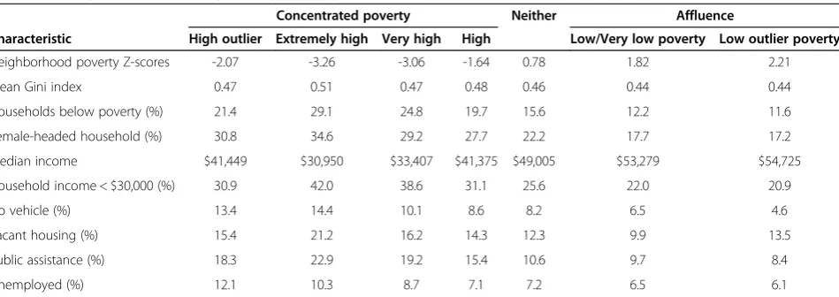
Measures of material disadvantage were associated with a greater degree of concentrated county poverty (Table 2). The proportion of households with incomes below the U.S. federal poverty line, headed by females, with incomes less than $30,000 per year, reporting no automobiles avail-able to the household, vacant housing, on public assist-ance and unemployed were all higher among counties with concentrated poverty (Table 2). Median household incomes ranged from $30,905 in counties with the highest degree of concentrated poverty to $53,279 in affluent counties. The Gini index, a measure of income inequality within a county, with higher values indicative of greater inequality [28], were slightly higher in poor counties.
Incident ESRD by county poverty category
Median follow up for our study was 6.0 years, and a total of 2,615 participants died during follow up. There were 158 incident cases of ESRD of follow up. Incident ESRD rates were 178.8 per 100,000 person-years (105py) (95% confidence interval [CI], 83.0 to 339.5/105py) among in-dividuals in high poverty outlier counties and were 76.3 /105py (95% CI 34.9 to 144.9/105py) in affluent outlier counties, p for trend = 0.06 (Figure 1). In unadjusted competing risk models, persons residing in high poverty outlier counties had higher incidence of ESRD (which was not statistically significant) when compared to those persons residing in counties with neither high poverty nor affluence [hazard ratio (HR) 1.54, 95% Confidence
Interval (CI) 0.75-3.20]. This association was markedly attenuated following adjustment for socio-demographic factors (age, sex, race, education, and income); HR 0.96, 95% CI 0.46-2.00. In this multivariable competing risk model, only income was independently associated with risk of ESRD [hazard ratio (HR) 3.75, 95% confidence interval (CI) (1.62-8.64) comparing the < $20,000 group to the > =$75,000 group] (Table 3). There were no statis-tically significant associations of county poverty with in-cident ESRD. Furthermore, there was no statistically significant interaction between income and county pov-erty category. We did not perform further adjustment of our models for other factors noted in Table 1, such as baseline kidney function, diabetes and hypertension sta-tus, out of concern for potentially inducing biased esti-mates [32].
Discussion
Among a population-based cohort of U.S. adults, we found that socio-demographic factors, including household in-come, varied in an expected direction across county pov-erty levels, and the county povpov-erty metric clearly defined levels of material disadvantage for this population. We re-port that the well-known association of low income with increased risk of ESRD is strong and independent of geospatially-linked measures of county poverty.
There are several potential explanations for our findings. First, we found that REGARDS participant characteristics well-known to be associated with poverty and CKD varied in an expected direction across geospatially-linked mea-sures of county poverty. We also found a non-statistically significant association between high poverty outlier coun-ties and higher incidence of ESRD in our unadjusted ana-lyses (Figure 1). However, the county poverty association
Table 2 County characteristics by county poverty levels (based on 2010 U.S. census data)
Concentrated poverty Neither Affluence
Characteristic High outlier Extremely high Very high High Low/Very low poverty Low outlier poverty
Neighborhood poverty Z-scores -2.07 -3.26 -3.06 -1.64 0.78 1.82 2.21
Mean Gini index 0.47 0.51 0.47 0.48 0.46 0.44 0.44
Households below poverty (%) 21.4 29.1 24.8 19.7 15.6 12.2 11.6
Female-headed household (%) 30.8 34.6 29.2 27.7 22.2 17.7 17.2
Median income $41,449 $30,950 $33,407 $41,375 $49,005 $53,279 $54,725
Household income < $30,000 (%) 30.9 42.0 38.6 31.1 25.6 22.0 20.9
No vehicle (%) 13.4 14.4 10.1 8.6 8.2 6.5 4.6
Vacant housing (%) 15.4 21.2 16.2 14.3 12.3 9.9 13.5
Public assistance (%) 18.3 22.9 19.2 15.4 10.6 9.7 8.4
Unemployed (%) 12.1 10.3 8.7 7.1 7.2 6.5 6.1
Note:P-values for all rows were <0.05. Categories of county poverty were defined as: high outlier poverty, extremely high poverty, very high poverty, high poverty,
178.8
164.3
137 135.5 116.7
109.1
76.3
0 50 100 150 200 250 300 350 400
High Outlier
Extremely High
Very High
High Neither Low Low
Outlier
Incident ESRD rate/100,000 person-years
County Poverty Category
Figure 1Incident ESRD rate/100,000 person years (95% confidence interval) by County Poverty Category.There were 158 ESRD cases during follow-up. Incident ESRD rates declined from 178.8 per 100,000 person-years (105py) in high poverty outlier counties to 76.3 /105py in affluent outlier counties, p trend = 0.06.
Table 3 Hazard ratios for incident ESRD by county poverty and individual household income accounting for the competing risk of mortality
Unadjusted Model 1* Model 2**
n = 23,314 n = 23,295 n = 23,295
ESRD, total events = 158
County poverty levels (number of ESRD events)
High outliers (8) 1.54 (0.75-3.20) 1.03 (0.50-2.13) 0.96 (0.46-2.00)
Extremely high (7) 1.36 (0.63-2.95) 1.20 (0.55-2.61) 1.10 (0.51–2.39)
Very high (13) 1.14 (0.63-2.05) 1.25 (0.69-2.28) 1.16 (0.64-2.10)
High (31) 1.13 (0.74-1.72) 1.09 (0.71-1.66) 1.04 (0.68-1.58)
Neither (76) Ref Ref Ref
Low and very low (14) 1.00 (0.56-1.76) 1.21 (0.69-2.14) 1.19 (0.68-2.10)
Low outliers (9) 0.68 (0.34-1.36) 1.00 (0.49-2.04) 1.01 (0.50-2.06)
Demographics
Age, years, continuous 1.02 (1.01-1.04) 1.02 (1.00-1.03)
Male 1.63 (1.19-2.22) 1.82 (1.34-2.49)
Black (compared to white) race 4.18 (2.89-6.06) 3.59 (2.47-5.23)
Socioeconomic status
Education < High School (H.S.) compared to > =H.S. 1.18 (0.78, 1.78) 0.98 (0.64-1.51)
Income category, %
Refused 2.17 (0.87-5.43)
<$20,000 3.75 (1.62-8.64)
$20,000 to <35,000 4.55 (2.04-10.13)
$35,000 to <75,000 1.56 (0.66-3.64)
≥$75,000 Ref
was almost entirely accounted for by differences in race and income (Table 3). Thus, constitutional factors (e.g. genetic background) and individual income may be far more potent predictors of ESRD than community SES. Second, the well-established and plausible association of community SES and health outcomes may vary for differ-ent patidiffer-ent populations. For example, in contrast to our findings, Merkinet al.reported that among male and fe-male adults 65 years and older, residence in a low SES area was associated with progressive CKD, however individual level income was not [13]. Notably, Merkinet al. found in a younger population that residence in a low SES area was independently associated with progressive CKD only among white men, with no significant associations documented for white women or African Americans [12]. Their findings also raise a third potential explan-ation for our study findings, which is that individual versus community resources may play different roles in different stages of CKD. One could envisage, for ex-ample, that community resources may play a greater role in early development of CKD via their influence on the development and management of key risk factors for CKD (e.g. type 2 diabetes that develops as a conse-quence of limited physical activity). However, a recent study by Gaskinet al.found that household poverty sta-tus, but not neighborhood poverty concentration, was independently associated with odds of having diabetes [33]. Thus individual income, as compared to commu-nity SES, may be a more important determinant of CKD risk factors as well as CKD progression.
Our findings have important implications. The Healthy People 2020 initiative, the U.S. national blueprint for pub-lic health goals, aims to eliminate socioeconomic health disparities among patients with kidney disease in the U.S. by 2020 [34]. Achieving this goal will require the identifi-cation of the root cause of socioeconomic disparities in CKD, as well as targeted public and clinical interventions to mitigate these disparities. The findings of our study support a focus on individual rather than community re-sources when attempting to reduce disparities in ESRD, and emphasize the need to prevent and better manage established CKD risk factors such as diabetes and hyper-tension among low income individuals.
Conclusions
Our study had limitations. First, not all participants’ resi-dences could be geocoded and many did not provide in-formation about their annual household income. Those who did not provide their incomes comprised a greater proportion of the participants residing in less affluent communities than they did those living in more affluent communities. We also found a non-statistically significant trend towards greater risk of ESRD in this population, compared to those reporting earning at least $75,000/year.
Second, our measure of annual household income did not take into account household size and therefore may have failed to classify individuals with larger household income and a large family as economically disadvantaged. There-fore, our estimates of the relation between income and ESRD are conservative. Third, the small number of ESRD events in certain county poverty categories may have lim-ited our power to detect statistically significant associa-tions. Fourth, we lacked a measure of SES across the life course [35] and participants may have changed residence (and potentially, county poverty category) during the follow-up period. Additionally, it is possible that advanced kidney disease could have led to economic disadvantage over the life course for some participants (ie. reverse causality). Fifth, the majority of participants in our study resided in the U.S.‘stroke belt’, thus our results may not be generalizable to other U.S. population samples. While we found that income was strongly and independently asso-ciated with risk of ESRD, an analysis of the Kidney Early Evaluation Program, a nationwide community-based screening study of persons at high risk of kidney disease, found that other measures of individual SES (education and health insurance) were not independently associated with incident ESRD [36]. Finally, and importantly, coun-ties may not be the optimal proxies for geography (e.g. they may be too large of an area) and our analysis is sub-ject to potential bias due to the modifiable areal unit prob-lem [37]. Neighborhood, census tract or ZIP code level poverty measures may have yielded different findings in our study. The limitations of our study are balanced by its large number of participants with well-balanced represen-tation of white and black adults, and this being the first study to examine the relative associations of individual and community SES with incident ESRD.
In conclusion, as compared to annual family income, geospatially-linked measures of community poverty have little relation with risk of ESRD. Efforts to mitigate so-cioeconomic disparities in CKD may be best appropri-ated at the individual level.
Competing interest
Funding for this study was provided by an investigator-initiated grant-in-aid from Amgen Corporation. Representatives from Amgen did not have any role in the design and conduct of the study, the collection, management, analysis, and interpretation of the data, or the preparation or approval of the manuscript.
Authors’contributions
DC and WM conceived of the study design, analyzed and interpreted the data, and drafted the manuscript. OG and DS contributed substantially to the interpretation of the data and revised the manuscript. SF and J-CL analyzed the data and contributed to the drafting of the manuscript. SJ and NP contributed to the interpretation of the data and revised the manuscript. All authors read and approved the final manuscript.
Acknowledgements
represent the official views of the National Institute of Neurological Disorders and Stroke or the National Institutes of Health. Representatives of the funding agency have been involved in the review of the manuscript but not directly involved in the collection, management, analysis or interpretation of the data. The authors thank the other investigators, the staff, and the participants of the REGARDS study for their valuable contributions. A full list of participating REGARDS investigators and institutions can be found at http://www.regardsstudy.org. The authors thank Dr. James B. Holt for his contributions to this manuscript. Dr. Crews was supported by the Harold Amos Medical Faculty Development Program of the Robert Wood Johnson Foundation, Princeton, NJ, grant K23DK097184 from the National Institute of Diabetes and Digestive and Kidney Diseases (NIDDK), Bethesda, MD and the Gilbert S. Omenn Anniversary Fellowship of the Institute of Medicine. Dr. Powe was supported, in part, by grant R01 DK78124 from the NIDDK. Publication of this article was funded in part by the Open Access Promotion Fund of the Johns Hopkins University Libraries.
Author details
1
Division of Nephrology, Department of Medicine, Johns Hopkins Medical Institutions, 301 Mason F. Lord Drive, Suite 2500, Baltimore, MD 21224, USA. 2
Welch Center for Prevention, Epidemiology and Clinical Research, Johns Hopkins Medical Institutions, Baltimore, MD, USA.3Division of Nephrology, Department of Medicine, University of Alabama Birmingham, Birmingham, AL, USA.4Department of Epidemiology, University of Alabama Birmingham, Birmingham, AL, USA.5Department of Epidemiology, Emory University, Atlanta, GA, USA.6Institute of Social and Preventive Medicine, Centre Hospitalier Universitaire Vaudois and University of Lausanne, Lausanne, Switzerland.7Department of Public Health Sciences, Loyola University Chicago, Maywood, IL, USA.8Department of Biostatistics, University of Alabama Birmingham, Birmingham, AL, USA.9Department of Medicine, San Francisco General Hospital, San Francisco, CA, USA.10Department of Medicine, University of California at San Francisco, San Francisco, CA, USA. 11
Department of Medicine, Emory University, Atlanta, GA, USA.
Received: 14 August 2014 Accepted: 27 November 2014 Published: 4 December 2014
References
1. Patzer RE, McClellan WM:Influence of race, ethnicity and socioeconomic status on kidney disease.Nat Rev Nephrol2012,8(9):533–541.
2. Galobardes B, Shaw M, Lawlor DA, Davey Smith G, Lynch J:Methods in Social Epidemiology 1st Edition.San Francisco: Jossey-Bass; 2006. 3. Coresh J, Wei GL, McQuillan G, Brancati FL, Levey AS, Jones C, Klag MJ:
Prevalence of high blood pressure and elevated serum creatinine level in the United States: findings from the third National Health and Nutrition Examination Survey (1988-1994).Arch Intern Med2001,161(9):1207–1216. 4. Robbins JM, Vaccarino V, Zhang H, Kasl SV:Socioeconomic status and type
2 diabetes in African American and non-Hispanic white women and men: evidence from the Third National Health and Nutrition Examination Survey.Am J Public Health2001,91(1):76–83.
5. Grabner M:BMI trends, socioeconomic status, and the choice of dataset. Obes Facts2012,5(1):112–126.
6. Martins D, Tareen N, Zadshir A, Pan D, Vargas R, Nissenson A, Norris K:The association of poverty with the prevalence of albuminuria: data from the Third National Health and Nutrition Examination Survey (NHANES III). Am J Kidney Dis2006,47(6):965–971.
7. Crews DC, Charles RF, Evans MK, Zonderman AB, Powe NR:Poverty, race, and CKD in a racially and socioeconomically diverse urban population. Am J Kidney Dis2010,55(6):992–1000.
8. McClellan WM, Newsome BB, McClure LA, Howard G, Volkova N, Audhya P, Warnock DG:Poverty and racial disparities in kidney disease: the REGARDS study.Am J Nephrol2010,32(1):38–46.
9. Volkova N, McClellan W, Klein M, Flanders D, Kleinbaum D, Soucie JM, Presley R:Neighborhood poverty and racial differences in ESRD incidence.J Am Soc Nephrol2008,19(2):356–364.
10. Crews DC, McClellan WM, Shoham DA, Gao L, Warnock DG, Judd S, Muntner P, Miller ER, Powe NR:Low income and albuminuria among REGARDS (Reasons for Geographic and Racial Differences in Stroke) study participants.Am J Kidney Dis2012,60(5):779–786.
11. Grace BS, Clayton P, Cass A, McDonald SP:Socio-economic status and incidence of renal replacement therapy: a registry study of Australian patients.Nephrol Dial Transplant2012,27(11):4173–4180.
12. Merkin SS, Coresh J, Diez Roux AV, Taylor HA, Powe NR:Area
socioeconomic status and progressive CKD: the Atherosclerosis Risk in Communities (ARIC) Study.Am J Kidney Dis2005,46(2):203–213. 13. Merkin SS, Roux AV, Coresh J, Fried LF, Jackson SA, Powe NR:Individual
and neighborhood socioeconomic status and progressive chronic kidney disease in an elderly population: The Cardiovascular Health Study. Soc Sci Med2007,65(4):809–821.
14. Hossain MP, Palmer D, Goyder E, El Nahas AM:Association of deprivation with worse outcomes in chronic kidney disease: findings from a hospital-based cohort in the United Kingdom.Nephron Clin Pract2012,120(2):c59–c70. 15. Shishehbor MH, Gordon-Larsen P, Kiefe CI, Litaker D:Association of
neighborhood socioeconomic status with physical fitness in healthy young adults: the Coronary Artery Risk Development in Young Adults (CARDIA) study.Am Heart J2008,155(4):699–705.
16. Bird CE, Seeman T, Escarce JJ, Basurto-Davila R, Finch BK, Dubowitz T, Heron M, Hale L, Merkin SS, Weden M, Lurie N:Neighbourhood socioeconomic status and biological‘wear and tear’in a nationally representative sample of US adults.J Epidemiol Community Health2010,64(10):860–865.
17. Mujahid MS, Diez Roux AV, Morenoff JD, Raghunathan TE, Cooper RS, Ni H, Shea S:Neighborhood characteristics and hypertension.Epidemiology
2008,19(4):590–598.
18. Pollack CE, Slaughter ME, Griffin BA, Dubowitz T, Bird CE:Neighborhood socioeconomic status and coronary heart disease risk prediction in a nationally representative sample.Public Health2012,126(10):827–835. 19. Diez-Roux AV:Multilevel analysis in public health research.Annu Rev
Public Health2000,21:171–192.
20. McClellan AC, Plantinga L, McClellan WM:Epidemiology, geography and chronic kidney disease.Curr Opin Nephrol Hy2012,21(3):323–328. 21. Howard VJ, Cushman M, Pulley L, Gomez CR, Go RC, Prineas RJ, Graham A,
Moy CS, Howard G:The reasons for geographic and racial differences in stroke study: objectives and design.Neuroepidemiology2005,25(3):135–143. 22. Warnock DG, McClellan W, McClure LA, Newsome B, Campbell RC, Audhya P,
Cushman M, Howard VJ, Howard G:Prevalence of chronic kidney disease and anemia among participants in the Reasons for Geographic and Racial Differences in Stroke (REGARDS) Cohort Study: baseline results.Kidney Int
2005,68(4):1427–1431.
23. Kurella Tamura M, Wadley V, Yaffe K, McClure LA, Howard G, Go R, Allman RM, Warnock DG, McClellan W:Kidney function and cognitive impairment in US adults: the Reasons for Geographic and Racial Differences in Stroke (REGARDS) Study.Am J Kidney Dis2008,52(2):227–234.
24. Levey AS, Stevens LA, Schmid CH, Zhang YL, Castro AF 3rd, Feldman HI, Kusek JW, Eggers P, Van Lente F, Greene T, Coresh J:A new equation to estimate glomerular filtration rate.Ann Intern Med2009,150(9):604–612. 25. Champion T, Coombes M, Openshaw S:A new definition of cities.Town
Ctry Plann1983,ᅟ:305–307.
26. Holt JB:The topography of poverty in the United States: a spatial analysis using county-level data from the Community Health Status Indicators project.Prev Chronic Dis2007,4(4):A111.
27. Diez Roux AV, Merkin SS, Arnett D, Chambless L, Massing M, Nieto FJ, Sorlie P, Szklo M, Tyroler HA, Watson RL:Neighborhood of residence and incidence of coronary heart disease.N Engl J Med2001,345(2):99–106. 28. Truman BI, Smith KC, Roy K, Chen Z, Moonesinghe R, Zhu J, Crawford CG,
Zaza S:Rationale for regular reporting on health disparities and inequalities - United States.MMWR Surveill Summ2011,60(Suppl):3–10. 29. Rural Health Research Center:Rural-Urban Commuting Area Codes (RUCAs).
http://www.depts.washington.edu/uwruca/ (Accessed 26 July 2012). 30. US Renal Data System:USRDS 2012 Annual Data Report: Atlas of End-stage Renal
Disease in the United States.Bethesda, MD: National Institutes of Health, National Institute of Diabetes and Digestive and Kidney Disease; 2012. 31. Fine JP, Gray RJ:A proportional hazards model for the subdistribution of
a competing risk.J Am Stat Assoc1999,94(446):496–509.
32. Glymour MM, Weuve J, Berkman LF, Kawachi I, Robins JM:When is baseline adjustment useful in analyses of change? An example with education and cognitive change.Am J Epidemiol2005,162(3):267–278.
33. Gaskin DJ, Thorpe RJ Jr, McGinty EE, Bower K, Rohde C, Young JH, Laveist TA, Dubay L:Disparities in diabetes: the nexus of race, poverty, and place.Am J Public Health2014,104(11):2147–2155.
34. US Department of Health and Human Services:National Healthcare Quality Report.http://www.ahrq.gov/qual/nhqr10/nhqr10.pdf (accessed May 5, 2013). 35. Shoham DA, Vupputuri S, Kaufman JS, Kshirsagar AV, Diez Roux AV, Coresh
socioeconomic conditions: the Atherosclerosis Risk in Communities (ARIC) study.Soc Sci Med2008,67(8):1311–1320.
36. Chang TI, Li S, Chen SC, Peralta CA, Shlipak MG, Fried LF, Whaley-Connell AT, McCullough PA, Tamura MK:Risk factors for ESRD in individuals with preserved estimated GFR with and without albuminuria: results from the Kidney Early Evaluation Program (KEEP).Am J Kidney Dis2013,
61(4 Suppl 2):S4–S11.
37. Openshaw S:The Modifiable Areal Unit Problem.Norwick: Geo Books; 2013.
doi:10.1186/1471-2369-15-192
Cite this article as:Crewset al.:Low income, community poverty and
risk of end stage renal disease.BMC Nephrology201415:192.
Submit your next manuscript to BioMed Central and take full advantage of:
• Convenient online submission
• Thorough peer review
• No space constraints or color figure charges
• Immediate publication on acceptance
• Inclusion in PubMed, CAS, Scopus and Google Scholar
• Research which is freely available for redistribution