Master’s Thesis by
Geert van der Wulp
Department of Econometrics & ORTilburg University
Supervisors and Thesis Committee Members
Prof. Dr. Bas Werker
Department of Econometrics & OR Department of Finance
Tilburg University
Drs. Roderick Molenaar
Research Department ABP Investments
Dr. Feike Drost
Department of Econometrics & OR Department of Finance
Tilburg University
Drs. Nolke Posthuma
Research Department ABP Investments
but not simpler.
Acknowledgments 3
1 Introduction 4
2 Introducing Copula Functions 6
2.1 De…nition of Copula Functions . . . 6
2.2 Sklar’s Theorem . . . 8
2.3 Copulas and Monotone Transformations . . . 11
2.4 Survival Copulas . . . 13
2.5 Copula Concordance and Fréchet Bounds . . . 14
2.6 The Product Copula . . . 16
3 Association Concepts 17 3.1 Introduction . . . 17
3.2 Independence and Perfect Dependence . . . 19
3.3 Measures of Concordance . . . 20
3.3.1 Kendall’s Tau . . . 21
3.3.2 Spearman’s Rho . . . 22
3.4 Measures of Dependence . . . 23
3.4.1 Schweizer and Wol¤’s Sigma . . . 23
3.4.2 Hoe¤ding’s Dependence Index . . . 23
3.5 Tail Dependence . . . 24
4 Copula Families 26 4.1 Introduction . . . 26
4.2 Elliptical Copulas . . . 28
4.2.1 Gaussian Copula . . . 28
4.2.2 t-Copula . . . 29
4.2.3 Kendall’s Tau and Spearman’s Rho . . . 30
4.2.4 Tail Dependence . . . 31
4.3 Archimedean Copulas . . . 34
4.3.1 De…nition and Properties . . . 34
4.3.2 Kendall’s Tau . . . 37
4.3.3 Tail Dependence . . . 37
4.3.4 Distribution Level Curves . . . 38
5 Copula Estimation 41 5.1 Introduction . . . 41
5.2 Exact Maximum Likelihood (EML) . . . 43
5.3 Inference Functions for Margins (IFM) . . . 44
5.4 Canonical Maximum Likelihood (CML) . . . 45
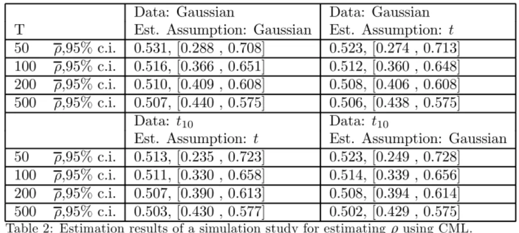
5.5 Applying CML to the Gaussian andt-copulas . . . 47
6.2 The Transformed Kendall’s Tau Estimator for½. . . 54
6.3 The Plug-in Estimator for§. . . 56
7 Simulation 58 7.1 General Simulation Algorithm . . . 58
7.2 Simulating from Gaussian andtCopulas . . . 60
7.3 Simulating from Archimedean Copulas . . . 62
8 Applications 67 8.1 Exchange Rates . . . 67
8.2 Hedge Fund Indices . . . 77
8.2.1 A Homogeneous Portfolio . . . 78
8.2.2 A Heterogeneous Portfolio . . . 82
8.3 Bonds . . . 86
Conclusions 94 Theory . . . 94
Practice . . . 96
Suggestions for further Research . . . 101
A 3D-graphs and Contour Plots 101 B Archimedean Copulas 123 C Tables 126 D Description Programs 132 D.1 CMLArchimedean.ox . . . 132
D.2 CMLElliptical.ox . . . 132
D.3 VaRArchimedean.ox . . . 132
D.4 VaRElliptical.ox . . . 133
D.5 VaREllipticalRolling.ox . . . 133
D.6 Marginalt.ox . . . 134
D.7 Sim1.ox . . . 134
This thesis was written at ABP Research in the period February 2003 until August 2003. Before I started studying papers about the main topic of this thesis, copulas, I was completely unfamiliar with that subject. Thanks to the help of my supervisors, Roderick Molenaar and Nolke Posthuma at the Research Department of ABP and Bas Werker from Tilburg University, I have been able to complete this ’test of competence’.
Furthermore I would like to thank all of the people at the Research Depart-ment for the interest that they have shown, and the advice that they have given me. Special thanks goes to Hindrik Angerman, who has put quite some time in explaining me basic and not so basic mathematics, and Frank van Weegberg, who has helped me collecting data on bond prices.
Furthermore I thank my friends at Tilburg University for the fun that we had and still have. Most of my gratitude however goes to my parents for their constant support over the years.
Naturally I take full responsibility for any errors, which will inevitably be present1.
1 Introduction
Traditionally the risk pro…les of …nancial products are estimated under the assumption of (joint) normality. The normal (Gaussian) distribution has all kinds of interesting and, especially from an asymptotical point of view, appeal-ing properties. Usappeal-ing normality assumptions makes life easier, because it often simpli…es calculations, it keeps results tractable, it makes sure that limit distri-butions can be given explicitly, etc. All those attractive properties have caused normality assumptions to form the foundation of many, historically invaluable, asset pricing theories such as Markowitz’ portfolio theory, the Capital Asset Pricing Model, and the Arbitrage Pricing Theory.
Yet it has been known for a long time that in …nance, probably more of-ten than not, normality assumptions are not very realistic. One of the earliest papers to report that wasMandelbrot 1963. Heavy tails and skewness are observed frequently for empirical distributions of return series. In order to make a thorough analysis of the risks associated with holding certain assets, deriva-tives, or portfolios thereof, this observed non-normal behavior of return series must be taken into account.
Financial practitioners regularly observe that in ’bear’ markets returns are more correlated than they are in ’bull’ markets. This asymmetry in return de-pendence can have a big in‡uence on the risk pro…le of a portfolio. If we make a risk pro…le simply assuming that there is a symmetric dependence relationship between returns, then we could be confronted with large portfolio losses much more often than we had expected. Therefore a basic question that has to be answered is: How to model the joint distribution of di¤erent risks?
A joint distribution can be seen as a framework containing two elements:
² All the marginal distributions.
² The dependence structure that exists between the marginal distribution functions.
A copula is a function that completely describes the dependence structure; it contains all the information to link the marginal distributions to their joint distribution. The theory allows one to combine several marginal distribution functions, possibly from di¤erent distributional families, with any copula func-tion and by doing so, obtaining a valid multivariate distribufunc-tion funcfunc-tion.
perfect dependence.
Section 3 deals with all kinds of association concepts, like independence, per-fect dependence, and tail dependence. There is also a treatment of the linear correlation coe¢cient. We explore in which situations it is useful to look at the linear correlation coe¢cient, and for which purposes it is unsuitable to use the linear correlation coe¢cient. Some alternative measures of association will be treated.
Section 4 discusses the two most commonly used parametric copula families, the elliptical copulas and the Archimedean copulas. Several characteristics of each of these families will be dealt with. The elliptical copula family includes the Gaussian copula and thet-copula.
Sections 5 and 6 describe parameter estimation techniques for copulas. The methods presented there will be based on the Maximum Likelihood Principle. Also we treat the application of these methods to the elliptical copulas, and the Archimedean copulas. Application of this technique to the class of Archimedean copulas is not straightforward. A method will be proposed to simplify matters.
Section 7 treats the topic of simulation, an important tool in …nance. Tech-nically speaking, simulating from copulas is not that di¢cult, if one is able to use the conditional sampling method. This method will be explained, as well as the reason why it is di¢cult to use this method in practice. For the Gaussian and t-copulas we will see a fast and accurate simulation algorithm. For the Archimedean copulas a recursive algorithm will be treated, but this will turn out to be a slow and inaccurate algorithm.
The Applications section, Section 8, shows the implementation of the copula techniques to various di¤erent portfolios. A portfolio of currencies, two portfo-lios with hedge fund indices, and two portfoportfo-lios with corporate bonds.
2 Introducing Copula Functions
2.1 De…nition of Copula Functions
Before de…ning what a copula function is, …rst a short introduction about the concept of a multivariate distribution function in general will be given. Let
X1; : : : ; Xnbe random variables, with marginal distribution functionsF1; : : : ; Fn,
respectively, and joint distribution functionH. The dependence structure of the variables is now completely described by the functionH in the following way:
H(x1; : : : ; xn) :=P[X1·x1; : : : ; Xn·xn]
Any of the marginal distribution functionsFican be obtained fromH, by letting xj ! 1for allj 6=i. The necessary and su¢cient properties of a multivariate
distribution function are (seeJoe 1997):
De…nition 1 (Multivariate or Joint Distribution Function)
A functionH:Rn ![0;1]is a multivariate distribution function if the following
conditions are satis…ed:
1. H is right continuous,
2. lim
xi!¡1H(x1; : : : ; xn) = 0, fori= 1; : : : ; n ,
3. lim
xi!1 8iH(x1; : : : ; xn) = 1,
4. For all (a1; : : : ; an) and (b1; : : : ; bn) with ai · bi for i = 1; : : : ; n the
following inequality holds:
2
X
i1=1 ¢ ¢ ¢
2
X
in=1
(¡1)i1+¢¢¢+inH(x
1i1; : : : ; xnin)¸0
wherexj1=aj and xj2=bj for all j.2
We now try to separate the joint distribution function H into its marginal distribution functions (the margins), and a part that describes the dependence structure. This means that somehow we will have to ’…lter out’ the information that is contained in all the margins. This can be established by the use of a probability integral transformation (sometimes also called a quantile transfor-mation).
H(x1; : : : ; xn) = P[X1·x1; : : : ; Xn ·xn]
= P[F1(X1)·F1(x1); : : : ; Fn(Xn)·Fn(xn)] = C(F1(x1); : : : ; Fn(xn))
2IfHhasn-th order derivatives, then this condition is equivalent to
@nH
Recall that if the random variableY has a continuous distribution functionF, thenF(Y)has aUniform(0,1)distribution. This implies that we have to de…ne the properties of the functionC, called the copula or the copula function, on a
set of standard uniformly distributed random variables. De…nition 2 (Copula Function)
An n-dimensional copula C is a function from [0;1]n to [0;1] satisfying the
following properties:
1. C(u1; : : : ; un) = 0 ifui= 0 for somei= 1; : : : ; n.
2. C(1; : : : ;1; ui;1; : : :1) =ui for allui2[0;1]:
3. For all (a1; : : : ; an) and (b1; : : : ; bn) with ai · bi for i = 1; : : : ; n the
following inequality holds:
2
X
i1=1 ¢ ¢ ¢
2
X
in=1
(¡1)i1+¢¢¢+inC(u
1i1; : : : ; unin)¸0 (1)
whereuj1=aj anduj2=bj for all j andujk 2[0;1]for allj andk.
Property 1 is also sometimes expressed as: ”Cis grounded”, and property 3 as: ”C isn-increasing3”. The properties that a function must have to be
quali-…ed as a copula function follow from the fact that it has to de…ne a distribution function with standard uniform margins. So how about continuity of the cop-ula? Next theorem ascertains the fact that any copula is uniformly continuous on its domain.
Theorem 3 (Copula Continuity)
LetC be anyn-copula. Then, for allu;v2[0;1]n;
jC(v)¡C(u)j · n
X
i=1
jvi¡uij
Proof. SeeSchweizer and Sklar 1983.
3The statement: ”Cis n-increasing”, is not equivalent with the statement: ”C is a
2.2 Sklar’s Theorem
In previous section the link between a joint distribution function and a copula has been explained intuitively. In this section it will be formalized mathemat-ically. That is done in the most important theorem regarding copulas, Sklar’s theorem.
Theorem 4 (Sklar’s Theorem)
LetHbe ann-dimensional distribution function with marginsF1; : : : ; Fn. Then
there exists ann-copula C such that for all x2Rn,
H(x1; : : : ; xn) =C(F1(x1); : : : ; Fn(xn)) (2)
If F1; : : : ; Fn are all continuous, then C is unique; otherwise C is uniquely
determined on Range(F1)£ ¢ ¢ ¢ £Range(Fn). Conversely, if C is an n-copula
andF1; : : : ; Fn are distribution functions, then the functionH de…ned above is
ann-dimensional distribution function with margins F1; : : : ; Fn.
Proof. SeeSklar 1996.
Sklar’s theorem states that for any continuous joint distribution function the univariate margins and the multivariate dependence structure can be separated. That is why a copula is interpreted as the dependence structure: the univariate margins do not contain any information about the dependence structure. We would also like to have an expression for the copula in terms of the margins and the joint distribution function. This can be derived directly as a corollary to Sklar’s theorem. Before doing that we will …rst need to de…ne the concept of a generalized inverse of a distribution function.
De…nition 5 (Generalized Inverse of a Distribution Function)
Let F be a univariate distribution function. Then the generalized inverse of F
is de…ned in the following way:
F¡1(t) := inffx2RjF(x)¸tg for allt2[0;1]
using the conventioninff;g:=¡1.
Now all tools are available to express the copula in terms of the joint distri-bution functionHand the marginsF1; : : : ; Fn.
Corollary 6 (Copula Representation)
LetH be ann-dimensional distribution function with continuousmargins F1; : : : ; Fn, and copulaC (satisfying Sklar’s theorem). Then for anyu2[0;1]n,
C(u1; : : : ; un) =H¡F1¡1(u1); : : : ; Fn¡1(un)¢ (3)
Example 7 (Bivariate Copula Representation)
Let X1 andX2 be random variables, jointly having a Gumbel bivariate logistic
distribution. That means
H(x1; x2) =¡1 +e¡x1+e¡x2¢¡1
The margins are: F1(x1) = lim
x2!1H(x1; x2) = (1 +e
¡x1)¡1 and F
2(x2) =
lim
x1!1H(x1; x2) = (1 +e
¡x2)¡1. Now we want to specify the copula
func-tionC on the transformed standard uniformly distributed variables u1 andu2.
From the transformations u1 = F1(x1) and u2 = F2(x2), we obtain that
F1¡1(u1) = ¡log¡u¡11¡1
¢ and
F2¡1(u2) = ¡log¡u¡21¡1
¢. Substitute this
into relationship (3) to obtain:
C(u1; u2) =
u1u2
u1+u2¡u1u2
Example 8 (Bivariate Gaussian Copula)
LetX1andX2be random variables, jointly having a bivariate standard Gaussian
distribution with a linear correlation coe¢cient½, i.e.
H(x1; x2) = ©½(x1; x2)
If we want to …nd the dependence structure between X1 and X2, then we can
again use relationship (3). The univariate margins of a multivariate standard Gaussian distribution are univariate standard Gaussian. So F1(x1) = © (x1)
andF2(x2) = © (x2). The transformation of variables therefore becomes: x1=
©¡1(u
1)andx2= ©¡1(u2). Inserting this into (3) yields us the representation
of a bivariate Gaussian copula with linear correlation coe¢cient½:
C½Ga(u1; u2) = ©½¡©¡1(u1);©¡1(u2)¢
In Example 8 we see that a multivariate Gaussian distribution is formed by combining a Gaussian copula with all univariate Gaussian marginals. I.e., if we combine the bivariate Gaussian copula CGa
½ (u1; u2) with the marginal
distributionsu1= ©
³x
1¡¹1 ¾1
´
andu2= ©
³x
2¡¹2 ¾2
´
, then we …nd:
H(x1; x2) = ©½
µ
©¡1
µ
©
µx
1¡¹1
¾1
¶¶
;©¡1
µ
©
µx
2¡¹2
¾2
¶¶¶
= ©½
µx
1¡¹1
¾1
;x2¡¹2 ¾2
¶
a bivariate Gaussian distribution with mean¹=
µ
¹1 ¹2
¶
, and variance-covariance
matrix§ =
µ
¾2
1 ½¾1¾2
½¾1¾2 ¾22
¶
So far we only described the copula distribution functions. Next, the concept of copula density functions is introduced. This will play a role in the parameter estimation methods for copulas that are based on the Maximum Likelihood Principle.
Corollary 9 (Copula Density)
The relationship between the multivariate density functionh(x1; : : : ; xn)and the
copula densityc, is given by:
h(x1; : : : ; xn) =c(F1(x1); : : : ; Fn(xn)) n
Y
i=1
fi(xi) (4)
Proof. Let h be the n-dimensional density function that belongs to the distribution functionH. De…nehby:
h(x1; : : : ; xn) =
@H(x1; : : : ; xn) @x1¢ ¢ ¢@xn
Now substitute (2), to obtain:
h(x1; : : : ; xn) =
@C(F1(x1); : : : ; Fn(xn)) @x1¢ ¢ ¢@xn
Using the substitutionui=Fi(xi)fori= 1; : : : ; nwe obtain:
h(x1; : : : ; xn) =
@C(u1; : : : ; un) @u1¢ ¢ ¢@un
n
Y
i=1
fi(xi)
= c(u1; : : : ; un) n
Y
i=1
fi(xi)
2.3 Copulas and Monotone Transformations
Assume that a researcher is interested in the joint distribution of several vari-ables. He collects data and, somehow, estimates the joint distribution function of the variables of interest. If the research is still in the modeling phase, then it often happens that a decision is taken to do a transformation on one or more variables. E.g., one of the variables is transformed logarithmically. How should the researcher proceed to obtain an estimate for the new joint distribution func-tion?
It turns out that for strictly monotone transformations of random variables, copulas are either invariant, or they change in a simple way. This corresponds with the idea of looking at the copula function as the dependence structure. Typically, the invariance of copulas holds under transformations that are all strictly increasing, as next theorem shows:
Theorem 10 (Copula Invariance)
Let (X1; : : : ; Xn)be a vector of continuous random variables having copula C.
If®1; : : : ; ®n are strictly increasing functions on Range(X1),. . . ,Range(Xn),
re-spectively, then(®1(X1); : : : ; ®n(Xn))also has copulaC.
Proof. From Embrechts et al. 2001b:
LetF1; : : : ; Fndenote the distribution functions ofX1; : : : ; Xn, and letG1; : : : ; Gn
denote the distribution functions of ®1(X1); : : : ; ®n(Xn). Let (X1; : : : ; Xn)
have copulaC and let(®1(X1); : : : ; ®n(Xn))have copulaC®. Then:
C®(G1(x1); : : : ; Gn(xn)) = P[®1(X1)·x1; : : : ; ®n(Xn)·xn] = P£X1·®¡11(x1); : : : ; Xn·®¡n1(xn)¤4 = C¡F1¡®¡11(x1)¢; : : : ; Fn¡®¡n1(xn)¢¢ = C(G1(x1); : : : ; Gn(xn))
Since X1; : : : ; Xn are continuous, Range(G1) = : : : =Range(Gn) = [0;1]. It
follows thatC®=C on[0;1]n.
The result of this theorem is that a logarithmic or any other strictly increas-ing transformation of one or more variables means that we only have to change the marginal distributions, not the copula function itself. So what will happen then if there is at least one transformation that is strictly decreasing? It turns out that the copula of the transformed data can be expressed in terms of the ’old’ copula and its margins.
4Since®
1; :::; ®nare all strictly increasing:Gi(y) =P(®i(Xi)·y) =P
³
Xi·®¡i1(y)
´
=
Fi
³
Theorem 11 Let (X1; : : : ; Xn) be a vector of continuous random variables
having copula CX1;:::;Xn. Let ®1; : : : ; ®n be strictly monotone functions on
Range(X1),. . . ,Range(Xn)respectively, and let(®1(X1); : : : ; ®n(Xn))have
cop-ula C®1(X1);:::;®n(Xn). Furthermore, let ®i be strictly decreasing for some i.
Without loss of generality, leti= 1. Then
C®1(X1);:::;®n(Xn)(u1; : : : ; un) =
C®2(X2);:::;®n(Xn)(u2; : : : ; un)¡CX1;®2(X2);:::;®n(Xn)(1¡u1; u2; : : : ; un)
Proof. SeeEmbrechts et al. 2001b.
Using the two above theorems recursively it can be shown that the copula
C®1(X1);:::;®n(Xn) can be expressed in terms of the copula CX1;:::;Xn and its
margins. This is shown for the bivariate case:
Example 12 Let ®1 be strictly decreasing and let ®2 be strictly increasing:
C®1(X1);®2(X2)(u1; u2) = u2¡CX1;®2(X2)(1¡u1; u2) = u2¡CX1;X2(1¡u1; u2)
Let®1 and®2 be strictly decreasing:
C®1(X1);®2(X2)(u1; u2) = u2¡CX1;®2(X2)(1¡u1; u2)
2.4 Survival Copulas
Sometimes in …nancial theory one is interested in the distribution of the remain-ing lifetime, or survival time, of objects. This is for instance the case in credit risk management, when modeling the times to default of a basket of credits. Assume that we have a portfolio ofndi¤erent securities, with stochastic times to defaultX1; : : : ; Xn. We want to have information about the joint distribution
of these times to default.
H(x1; : : : ; xn) :=P[X1> x1; : : : ; Xn> xn]
This is called the ’joint survival function’. Assuming that we already found the copula CX1;:::;Xn forH, how to obtain then the copula Cb, the survival copula
for H? For that we can use the results derived in the previous section. Use Theorem 11, with ®i(y) = 1¡y for all i, to expressCb in terms of CX1;:::;Xn
and its univariate margins. This is shown again for the bivariate case: Example 13 (Bivariate Survival Copula)
b
C(u1; u2) = C1¡X1;1¡X2(u1; u2) = u2¡CX1;1¡X2(1¡u1; u2)
= u2¡(1¡u1¡CX1;X2(1¡u1;1¡u2)) = u1+u2¡1 +CX1;X2(1¡u1;1¡u2)
A second concept that is often used in the literature is the notion of a joint survival function C for uniform random variables having a joint distribution function given by the copulaC.
C(u1; : : : ; un) = H(u1; : : : ; un)
= P[U1> u1; : : : ; Un> un]
The link between the joint survival function C and the survival copula Cb is given by:
C(u1; : : : ; un) =Cb(1¡u1; : : : ;1¡un)
This link is established for the bivariate case in the next example. Example 14 (Bivariate Joint Survival Function)
C(u1; u2) = P[U1> u1; U2> u2]
= 1¡(P[U1·u1][P[U2·u2])
= 1¡(P[U1·u1] +P[U2·u2]¡P[U1·u1; U2·u2])
= 1¡u1¡u2+C(u1; u2)
2.5 Copula Concordance and Fréchet Bounds
In comparing copulas, the concept of concordance ordering is often used: De…nition 15 (Concordance Ordering of Copulas)
CopulaC1 is said to be smaller than copula C2,C1ÁC2, if:
C1(u)·C2(u), for allu2[0;1]n
The partial ordering of the copulas is called a concordance ordering5. Not
every pair of copulas can be ordered using this concept. However, a lot of parametric copula families are totally ordered. A one-parameter family fC®g
is called positively ordered ifC®1 ÁC®2 whenever®1·®2. Using the
concor-dance ordering, copulas are bounded. De…nition 16 (Fréchet Bounds)
De…ne on[0;1]n the functionsC¡ andC+ as:
C¡(u1; : : : ; un) : = max
à n X
i=1
ui¡n+ 1;0
!
C+(u
1; : : : ; un) : = min (u1; : : : ; un)
The de…ned functions are called, respectively, the lower and the upper Fréchet bound.
The lower and upper Fréchet bound will play an important role in the theory of dependence structures. They will form the mathematical de…nitions of the concepts ’perfectly negatively dependent’ and ’perfectly positively dependent’. Theorem 17 (Fréchet-Hoe¤ding Bounds Inequality)
LetC be anyn-copula, then:
C¡ÁCÁC+
Proof. The upper bound:
C(u1; : : : ; un) = P(U1·u1; : : : ; Un·un) · min
i=1;:::;nP(Ui·ui)
= min
i=1;:::;nui = C+(u
1; : : : ; un)
The lower bound:
C(u1; : : : ; un) = P(U1·u1; : : : ; Un·un)
= P
à n \
i=1
fUi·uig
!
= 1¡P
à n [
i=1
fUi > uig
!
(DeMorgan’s Law)
¸ 1¡ n
X
i=1
P(Ui> ui)
= 1¡
n
X
i=1
(1¡ui)
= 1¡n+ n
X
i=1
ui
Because C(u1; : : : ; un)de…nes a probability it should be non-negative. Other
steps follow from the fact thatUi »Uniform(0,1).
C+ is an n-copula in all dimensions, but it can be shown, seeEmbrechts
et al. 2001b, that C¡ is not a copula forn¸3. In spite of that, C¡ is the
best possible lower bound, because of the next theorem: Theorem 18 (Attainability Lower Fréchet Bound)
For anyn¸3 and anyu2[0;1]n, there is ann-copula C (which depends onu)
such that
C(u) =C¡(u)
Proof. SeeNelsen 1999.
In appendix A, Figures A1 and A2, the 3-D graphs of the bivariate C+
andC¡ are drawn. Another, more common, way to display bivariate copulas is by drawing the contour diagram. This means that we connect all points
(u1; u2)having the same value forC(u1; u2). We do this for several …xed values
ofC(u1; u2). By plotting those lines in the(u1; u2)-plane we get an idea of how
2.6 The Product Copula
Previous subsection featured the Fréchet bounds, which will serve as the de…n-ition in copula terms of perfectly positively dependent and perfectly negatively dependent. We will now see their pendant, the product copula, which will serve as the mathematical formulation for independence.
De…nition 19 (Product Copula)
De…ne on[0;1]n the functionC? , called the product copula, as:
C?(u) =u1¢ ¢ ¢un
3 Association Concepts
3.1 Introduction
In practice, if people want to say something about the degree of association between two random variables, they often report the linear correlation coe¢cient between those variables.
De…nition 20 (Linear Correlation Coe¢cient)
Let (X; Y) be a vector of random variables with nonzero and …nite variances.
The linear correlation coe¢cient (also called Pearson’s correlation) for(X; Y)
is equal to:
½(X; Y) = p Cov(X; Y) V ar(X)pV ar(Y)
While½(X1; X2)is often used in practice as an indicator for dependence, it
is not up to that task in a lot of situations. This is mainly caused by the fact that½(X1; X2)is a strictly linear concept. An extensive theoretical treatment
of the de…ciencies of linear correlation can be found in Embrechts et al. 2001b. The same discussion can be found in Embrechts et al. 1999, but this time more focus is placed on practical issues.
A few reasons why linear correlation might not be the right measure of association to use as an indicator for dependence are:
1. Perfect positive dependence between risks does not necessarily imply that their correlation will be 1. Also, perfect negative dependence between risks does not necessarily imply that the correlation will be -1.
2. Zero correlation does not imply independence of risks.
3. Correlation is not invariant under all increasing transformations of the risks. E.g.,log (X)and log (Y)will generally have a di¤erent correlation
thanXandY.
Zero correlation only implies independence in case of a (multivariate) nor-mal distribution. In this section we …rst de…ne the concept of independence and perfect dependence in a copula setting. After that, three di¤erent forms of association measures will be treated: concordance measures, dependence mea-sures, and tail dependence measures. The …rst two are used to describe the joint behavior of two variables in general, while the last one is used to describe the joint behavior of extreme events.
variable. Concordance measures are able to locate nonlinear associations be-tween the variables that linear correlation might miss completely.
The main advantage of a measure of dependence over a measure of concor-dance is that it gives usproof of a functional dependence between two variables. A measure of dependence equals 0if and only if two variables are independent. A measure of dependence equals 1 if and only if each of the two variables is almost surely6 a strictly monotone function of the other.
A measure of concordance equals -1 or 1 if the two variables are perfectly dependent. Also a measure of concordance equals 0 whenever two variables are independent. However, these relationships do not hold the other way around! So a value of -1, 0, or 1 is no proof of the fact that variables are independent or perfectly dependent.
The main advantage of a measure of concordance over a measure of depen-dence is that it tells us something about the nature of the association between the variables. A measure of dependence ’only’ tells us that two variables are functionally dependent on one another. A measure of concordance also tells us if two variables tend to be high or low simultaneously, or that they tend to deviate in opposite directions.
In this section the two most commonly used association measures, Kendall’s tau and Spearman’s rho, will be presented. We will also look at two commonly used measures of dependence, namely Schweizer and Wol¤’s sigma and Hoe¤d-ings dependence index.
6A condition holds almost surely if it holds with probability 1, or equivalently, if it holds
3.2 Independence and Perfect Dependence
The most distinct levels of association between random variables are the situa-tions of independence and of perfect dependence. FormallyX1; : : : ; Xnare
inde-pendent if and only ifh(x1; : : : ; xn) =f1(x1)¢ ¢ ¢fn(xn)for allx1; : : : ; xn 2R,
whereh(x1; : : : ; xn)is the joint density function ofx1; : : : ; xn andfi(xi)is the
density function ofxi. Next theorem de…nes independence in copula terms.
Theorem 21 (Independence and the Product Copula)
LetX1; : : : ; Xnbe continuous random variables having copulaC, thenX1; : : : ; Xn
are independent if and only ifC=C?.
Proof. This follows directly from Sklar’s theorem combined with the de…n-ition of independence.
Two variables,XandY are perfectly dependent if each of the variables is a monotone function of the other variable. This de…nition can be formulated using the copula concepts of comonotonicity and countermonotonicity. The concept of comonotonicity and countermonotonicity are equivalent to ”perfect positive dependence” and ”perfect negative dependence” respectively.
De…nition 22 (Comonotonicity or Perfect Positive Dependence)
The random variablesXand Y are comonotonic if they have the copulaC+.
Theorem 23 (Comonotonicity or Perfect Positive Dependence)
X andY are comonotonic if and only if
(X; Y)= (uD (Z); v(Z))
for some random variable Z and u and v increasing functions. If X and Y
are continuous, then comonotonicity is equivalent toY =T(X) a.s. for some strictly increasing functionT.
Proof. SeeDe Matteis 2001.
De…nition 24 (Countermonotonicity or Perfect Negative Dependence) The random variables X andY are countermonotonic if they have the copula
C¡.
Theorem 25 (Countermonotonicity or Perfect Negative Dependence)
X andY are countermonotonic if and only if
(X; Y)= (uD (Z); v(Z))
for some random variableZ withuan increasing andva decreasing function. If XandY are continuous, then countermonotonicity is equivalent toY =T(X)
a.s. for some strictly decreasing functionT.
3.3 Measures of Concordance
Let(x1; y1)and(x2; y2)be two observations from a vector(X; Y)of continuous
random variables. Then the the pairs(x1; y1)and(x2; y2)are called concordant
if (x1¡x2) (y1¡y2) > 0, and discordant if (x1¡x2) (y1¡y2) < 0. First a
de…nition of a measure of concordance will be given. De…nition 26 (Measure of Concordance)
A numeric measure·of association between two continuous random variablesX
andY whose copula isCis a measure of concordance if it satis…es the following properties:
1. ·is de…ned for every pair X,Y of continuous random variables.
2. ¡1 =·X;¡X··C ··X;X = 1.
3. ·X;Y =·Y;X.
4. If X andY are independent, then·X;Y =·C? = 0.
5. ·¡X;Y =·X;¡Y =¡·X;Y.
6. If C1ÁC2, then ·C1··C2.
7. If f(Xn; Yn)gis a sequence of continuous random variables with copulas Cn, and iffCngconverges pointwise toC, thennlim
!1·Cn =·C.
Criterion number 6 for measures of concordance is the reason why the rela-tionship ”Á”, de…ned in De…nition 15, is called the concordance ordering. From the properties above we can derive the following link between monotone func-tional dependence of two variables and the value of their concordance measure: Theorem 27 Let · be a measure of concordance for continuous random vari-ablesX andY.
1. If Y is almost surely an increasing function ofX, then ·X;Y =·C+= 1.
2. IfY is almost surely a decreasing function ofX, then·X;Y =·C¡ =¡1.
3. If ® and¯ are strictly monotone functions on Range(X) and Range(Y), respectively, then·®(X);¯(Y)=·X;Y.
3.3.1 Kendall’s Tau
De…nition 28 (Kendall’s Tau)
Let(X1; Y1)and(X2; Y2)be two independent and identically distributed random
vectors. Then Kendall’s tau between the random variablesX andY is de…ned as:
¿X;Y =P[(X1¡X2) (Y1¡Y2)>0]¡P[(X1¡X2) (Y1¡Y2)<0]
As can be seen from the de…nition, Kendall’s tau is de…ned as the probability of concordance minus the probability of discordance for a pair of observations
(xi; yi)and(xj; yj). Looking at an observed sample with sample sizen, there are
¡n
2
¢distinct pairs
(xi; yi) and(xj; yj). Let cdenote the number of concordant
pairs, and d the number of discordant pairs in the sample. Then a sample
estimator for Kendall’s tau is given by7:
b
¿ = c¡d c+d
= c¡¡nd
2
¢
=
µn
2
¶¡1X
i<j
sign[(Xi¡Xj) (Yi¡Yj)]
So far we have not seen how Kendall’s tau between two variables can be linked to the copula function that describes their dependence structure. Next theorem establishes the general formula for calculation of Kendall’s tau from the copula function.
Theorem 29 (Kendall’s Tau)
Kendall’s tau for a vector of continuous random variables(X; Y)with copulaC
is given by:
¿X;Y = 4
Z Z
[0;1]2
C(u; v)dC(u; v)¡1 (5)
Proof. SeeDe Matteis 2001.
Calculation of this integral is not always straightforward, but fortunately for a lot of copulas this relationship can be simpli…ed.
7Note that the given relationship holds only if we ignore the possibility of ’ties’ occuring.
3.3.2 Spearman’s Rho De…nition 30 (Spearman’s Rho)
Let(X1; Y1),(X2; Y2)and(X3; Y3)be three independent and identically
distrib-uted random vectors. Then Spearman’s rho between the variables X andY is de…ned as:
%X;Y = 3 (P[(X1¡X2) (Y1¡Y3)>0]¡P[(X1¡X2) (Y1¡Y3)<0])
A sample estimator for Spearman’s rho is given by:
b%= 12 n(n2¡1)
n
X
i=1
µ
rank(Xi)¡n+ 1 2
¶ µ
rank(Yi)¡n+ 1 2
¶
where the rank of an observation denotes its position in an ordered sample:
rank(Xi) := 1 + #fjjXj< Xig+1
2#fjjj 6=i andXj=Xig (6)
Once again this can be expressed in terms of copulas. Theorem 31 (Spearman’s Rho)
Spearman’s rho for a vector of continuous random variables(X; Y)with copula
C is given by:
%X;Y = 12
Z Z
[0;1]2
uvdC(u; v)¡3
The de…nition of Spearman’s rho can be interpreted as the probability of concordance minus the probability of discordance for two vectors(X1; Y1)and
(X2; Y3). I.e., a pair of vectors with equal margins, but one vector has joint
distribution function H, and the other vector has independent components. Consequently Spearman’s rho intuitively measures the distance between the copulaC and the copula of independenceC?. In other words, Spearman’s rho
measures ’how close to independence the relationship between the two variables is’. This is formalized mathematically (SeeDe Matteis 2001):
%X;Y = 12
Z Z
[0;1]2
3.4 Measures of Dependence
De…nition 32 (Measure of Dependence)A numeric measure±of association between two continuous random variablesX
andY whose copula isC is a measure of dependence if it satis…es the following properties:
1. ± is de…ned for every pairX,Y of continuous random variables. 2. ±X;Y =±Y;X.
3. 0·±X;Y ·1.
4. ±X;Y = 0 if and only ifX andY are independent.
5. ±X;Y = 1 if and only if each of X and Y is almost surely a strictly
monotone function of the other.
6. If®and¯are almost surely strictly monotone functions on Range(X)and Range(Y), respectively, then±®(X);¯(Y)=±X;Y.
7. If f(Xn; Yn)gis a sequence of continuous random variables with copulas Cn, and iffCngconverges pointwise toC, then lim
n!1±Cn=±C.
Intuitively it is clear that measures of dependence are based on a ’distance’ between the copula of(X; Y)and the product copula C?.
3.4.1 Schweizer and Wol¤’s Sigma De…nition 33 (Schweizer and Wol¤’s Sigma)
Schweizer and Wol¤’s Sigma for a vector of continuous random variables(X; Y)
with copulaC is given by:
¾X;Y = 12
Z Z
[0;1]2
jC(u; v)¡uvjdudv
Notice from this de…nition the similarity with Spearman’s rho. The di¤er-ence between the two is that this measure reports the absolute distance between the copula under consideration and the product copula whereas Spearman’s rho reports the ’signed’ distance.
3.4.2 Hoe¤ding’s Dependence Index De…nition 34 (Hoe¤ding’s Dependence Index)
Hoe¤ding’s Dependence Index for a vector of continuous random variables(X; Y)
with copulaC is given by:
©2X;Y = 90
Z Z
[0;1]2
3.5 Tail Dependence
The treated measures of concordance and dependence tell us something about the joint behavior of two variables over their complete outcome space. But let’s assume that we are especially interested in the behavior of the joint distribution of two variables in the tails of the distribution. This is the case, for instance, when we calculate the Value at Risk of a portfolio.
Generally speaking, if we are interested in extreme portfolio returns, then we should focus on the joint extreme behavior of the univariate returns. The ’general joint behavior’ of two variables can be described by Kendall’s tau or Spearman’s rho. Joint tail events are described by coe¢cients of tail depen-dence. There are two cases of tail dependence, upper tail dependence, the joint occurrence of high return values, and lower tail dependence, the joint occurrence of low (typically negative) return values.
De…nition 35 (Upper Tail Dependence)
Let X and Y be random variables with distribution functions F and G. The coe¢cient of upper tail dependence betweenX andY is:
lim s%1P
£
Y > G¡1(s)jX > F¡1(s)¤=¸u
provided a limit ¸u 2[0;1]exists. If ¸u 2(0;1], thenX and Y are said to be
asymptotically dependent in the upper tail. If ¸u = 0 they are asymptotically
independent in the upper tail.
Next we will see how upper tail dependence can be represented in a cop-ula terms. Assuming the limits exist, a copcop-ula de…nition for the upper tail dependence is derived in the following way:
¸u = lim s%1P
£
Y > G¡1(s)jX > F¡1(s)¤
= lim
s%1
P£Y > G¡1(s); X > F¡1(s)¤
P[X > F¡1(s)]
= lim
s%1
C(s; s) 1¡s
To see how we perform these calculations in practice an example is treated for the Gumbel-Hougaard copula8.
Example 36 Suppose we have a bivariate Gumbel-Hougaard copula,
C®GH(u; v) = exph¡[(¡logu)®+ (¡logv)®]®1i for®2[1;1)
then the coe¢cient of upper tail dependence is equal to:
¸u = lim s%1
C(s; s) 1¡s
= lim
s%1
1¡2s+C(s; s) 1¡s
= lim
s%1
1¡2s+ exph¡[(¡logs)®+ (¡logs)®]®1i
1¡s
= lim
s%1
1¡2s+ exph2®1 logs
i
1¡s
= lim
s%1
1¡2s+s21=® 1¡s
9 = lim
s%1
¡2 + 21=®s21=®¡1 ¡1 = 2¡21=®
Thus for® >1,CGH
® has upper tail dependence. Because ®2[1;1), it follows
that¸GHu 2[0;1).
Lower tail dependence is used more often in practice, since it gives a lot of insight in the …nancial risks that we take by holding a certain portfolio of assets. De…nition 37 (Lower Tail Dependence)
Let X and Y be random variables with distribution functions F and G. The coe¢cient of lower tail dependence betweenX andY is:
lim s&0P
£
Y ·G¡1(s)jX·F¡1(s)¤=¸
l
provided a limit ¸l 2[0;1] exists. If ¸l 2 (0;1], then X and Y are said to be
asymptotically dependent in the lower tail. If ¸l = 0 they are asymptotically
independent in the lower tail.
Also lower tail dependence can be de…ned using copulas:
¸l = lim s&0P
£
Y ·G¡1(s)jX·F¡1(s)¤
= lim
s&0
P£Y ·G¡1(s); X ·F¡1(s)¤
P[X·F¡1(s)]
= lim
s&0
C(s; s) s
9This relationship follows from L’Hôpital’s Rule: lim x!a
f(x)
g(x) = limx!a
f0(x)
4 Copula Families
4.1 Introduction
This section will deal mainly with parametric copulas. The speci…c inclusion of the word ’parametric’ suggests that there is also something like non-parametric copulas, and indeed this is the case. Despite the fact that this thesis will not use such copulas in the practical section, it is useful to understand some of their basics. Three di¤erent forms of non-parametric copulas are distinguished in the current literature. The so-called Deheuvels or empirical copula, the kernel approximations to copulas, and copula approximations.
Deheuvels copula functions were introduced by Deheuvels 1979 and are sometimes also called empirical copulas. The empirical copula function is de-…ned similar to an empirical distribution function, by counting the number of outcomes below certain values and dividing that number by the total number of outcomes. Empirical copulas are used in practice, but have the disadvantage that they are discontinuous functions.
Kernel approximations to copula functions were introduced very recently in Fermanian and Scaillet 2003. No other papers had appeared about this approach when this thesis was written.
Approximations to copulas were introduced in Li et al. 1997. In this approach an approximating functional form for the copula is speci…ed. This approximation formula includes the empirical copula. Two important approxi-mating forms are called the Bernstein polynomial, and the checkerboard copula. A drawback is that, although these approximations do converge to the true cop-ula when the number of observations increases, the tail dependence will always equal zero for the approximations, as proven in Durrleman et al. 2000b. This paper suggests using a perturbation method to modify the copula approx-imation in such a way that the desired tail dependence can be introduced.
This thesis will only look at copula families that are parametric. That is the most commonly used approach in the literature. Because of the speci…c nature of this research, multivariate distributions of order higher than two, only two speci…c classes of parametric copulas will be treated. The extension of two-dimensional copulas to copulas of higher dimension is certainly not a trivial one, but for the two classes treated here it is feasible. Unfortunately there is still not so much literature to be found about copulas of order higher than two. Other classes of copulas can be found in the literature, such as the Fréchet Family (See Hürlimann 2001) and Extreme Value copulas (SeeJoe 1997).
using Sklar’s theorem. Deriving Gaussian andt-copulas with more than two dimensions is done equivalently to the bivariate case (See example 8). However, the class of elliptical copulas has an unfavorable property when talking about application in the …eld of …nance. The dependence structure is such that some ’stylized facts’ in …nancial data cannot be represented correctly. For instance, as already mentioned in the Introduction, the asymmetry of the lower and up-per tail of a distribution cannot be described proup-perly by an elliptical copula. This is because elliptical copulas exhibit ’radial symmetry’. A radial symmetric bivariate copula is a copula which has the property thatC(u; v) =C(v; u)and
C(u; v) =Cb(u; v) =u+v¡1+C(1¡u;1¡v). Another fact that is sometimes mentioned as a drawback of elliptical copulas is that they do not have closed form expressions.
4.2 Elliptical Copulas
4.2.1 Gaussian CopulaThe Gaussian copula is obtained by ’…ltering out’ all univariate Gaussian distri-butions from the multivariate Gaussian distribution. This is done by applying Sklar’s theorem, see Example 8. Here we will look at the general multivariate Gaussian copula of dimensionn.
De…nition 38 (Multivariate Gaussian Copula)
Let©denote the standard univariate Gaussian distribution function and let©n
§
denote the standard multivariaten-dimensional Gaussian distribution function with linear correlation matrix §. The n-dimensional Gaussian copula is then
de…ned as:
C§Ga(u1; : : : ; un) = ©n§
¡
©¡1(u1); : : : ;©¡1(un)¢
Here we observe a drawback of the elliptical copulas in general. They have no closed form expression. The de…nition above uses the Gaussian distribution function and inverse distribution function. Equivalently, the following de…nition is often used:
De…nition 39 (Multivariate Gaussian Copula)
Then-dimensional Gaussian copula with linear correlation matrix §is de…ned as:
CGa
§ (u1; : : : ; un) =
©¡1(u 1)
Z
¡1 ¢ ¢ ¢
©¡1(u n)
Z
¡1
exp¡¡!>§¡1!=2¢
j§j(2¼)n=2 d!n¢ ¢ ¢d!1
wherej§jstands for the determinant of §and!= (!1; : : : ; !n):
Parameter estimation for this copula will be done using methods based on maximum likelihood. Therefore we need an expression for the Gaussian copula density, which is provided by next theorem.
Theorem 40 (Gaussian Copula Density)
The copula density for a multivariate Gaussian copula is given by:
cGa§ (u1; : : : ; un) = 1 j§j1=2exp
µ
¡12!>¡§¡1¡I¢!
¶
(8)
where!= (!1; : : : ; !n) =¡©¡1(u1); : : : ;©¡1(un)¢.
Proof. Use relationship (4) and insert the multivariate Gaussian distribu-tion funcdistribu-tion and the univariate Gaussian density funcdistribu-tions to obtain:
1
(2¼)n=2j§j1=2exp
µ
¡12x>§¡1x ¶
=c(© (x1); : : : ;© (xn))
à n Y i=1 1 p 2¼exp µ
¡12x2i
Now we write out the product and transform the variables: ui = © (xi), i = 1; : : : ; n, …nding:
cGa§ (u1; : : : ; un) =
1
(2¼)n=2j§j1=2exp
¡
¡1
2!>§¡1!
¢
1 (2¼)n=2exp
¡
¡12!>!
¢
where ! = (!1; : : : ; !n) =¡©¡1(u1); : : : ;©¡1(un)¢. After getting rid of the
redundant terms and some rearranging we are left with the above expression.
In the appendix, Figures A7a, A7b, and A7c, the contour plots for the den-sity of the bivariate Gaussian copula can be found. For½= 0.2, 0.5 and 0.810
a few values of the density are plotted. When½tends to 1, the density will be
very close to the lineu1=u2. Note that if the correlation coe¢cients would be
negative, then the plots would all rotate over 90±.
We have already seen in example 8 that a multivariate Gaussian distrib-ution is formed by combining a Gaussian copula with all univariate Gaussian marginals.
4.2.2 t-Copula
Thet-copula is obtained by by ’…ltering out’ all univariatetº-distributions from
the multivariatet§;º-distribution. Again, this follows directly from Sklar’s
the-orem.
De…nition 41 (Multivariate t-Copula)
Let tº denote the univariate t-distribution function with º degrees of freedom,
and lett§;º denote the standard multivariaten-dimensionalt-distribution
func-tion with linear correlafunc-tion matrix§and degrees of freedomº. Then-dimensional
t-copula is then de…ned as:
C§t;º(u1; : : : ; un) =t§;º¡tº¡1(u1); : : : ; t¡º1(un)¢
Equivalently, the following de…nition is often used: De…nition 42 (Multivariate tCopula)
Then-dimensionalt-copula with linear correlation matrix§and degrees of free-domº, is de…ned as:
C§t;º(u1; : : : ; un) = t¡1
ºZ(u1)
¡1 ¢ ¢ ¢
t¡1 ºZ(un)
¡1
¡ ((º+n)=2)¡1 +!>§¡1!=º¢¡(º+n)=2
j§j1=2¡ (º=2) (º¼)n=2 d!n¢ ¢ ¢d!1
where j§j stands for the determinant of §, ! = (!1; : : : ; !n) and ¡ (¢) is the
Gamma function.
10Where½is the linear correlation. Here§ =· 1 ½
½ 1
¸
Using similar steps as for the Gaussian copula, we can derive the correspond-ing density for thet-copula:
Theorem 43 (t Copula Density)
The copula density for a multivariatet-copula is given by:
ct§;º(u1; : : : ; un) =
¡ ((º+n)=2) [¡ (º=2)]n¡1¡1 +!>§¡1!=º¢¡(º+n)=2
j§j1=2[¡ ((º+ 1)=2)]n Qn i=1
(1 +!2
i=º)¡
(º+1)=2
where!= (!1; : : : ; !n) =¡t¡º1(u1); : : : ; t¡º1(un)¢.
In the appendix, Figures A8a, A8b, and A8c, several contour plots can be found for a bivariate t8 copula. For½ = 0.2, 0.5 and 0.8 a few values of the
density are plotted. Note that if the number of degrees of freedom for the copula goes to in…nity, thet-copula will converge to a Gaussian copula (with equal§).
If the correlation coe¢cients would be negative, then the plots would all rotate over 90±.
A multivariate t-distribution is formed by combining a t-copula with all univariatet distributed marginals. It is not di¢cult to see that if we take the limit of at-copula forº ! 1, that we will end up having a Gaussian copula.
4.2.3 Kendall’s Tau and Spearman’s Rho
The most often-used measures of concordance are Kendall’s tau and Spearman’s rho. In an ideal situation we prefer to have a copula family for which those two measures can stretch over the complete interval[¡1;1]. For the Gaussian and t-copulas the following result concerning Kendall’s tau can be derived:
Theorem 44 (Kendall’s Tau for Gaussian and tCopulas)
Let (X1; : : : ; Xn) have copula C, where C is either a Gaussian or a t-copula.
Then for alliandj 2 f1; : : : ; ng
¿Xi;Xj = 2
¼arcsin½ij (9)
where½ij denotes the linear correlation coe¢cient between Xi andXj.
Proof. For a proof of an extended version of this theorem see Lindskog et al. 2001.
This result shows us that for elliptical copulas11, Kendall’s tau is a
trans-formation of the linear correlation coe¢cient. Also the theorem implies that
11The Theorem is applied here only to the Gaussian andt-copulas, but it is valid for all
for the Gaussian and t-copula, Kendall’s tau can cover the complete interval
[¡1;1]. For Spearman’s rho the relationship is more complicated. In Hult and Lindskog 2001it is proven that Spearman’s rho is not invariant in the class of elliptical distributions with continuous univariate margins and a …xed covariance matrix. Therefore, when measuring the degree of concordance in the data and in the theoretical copulas, people in general only use Kendall’s tau. For the sake of completeness a result for the Gaussian case is included.
Theorem 45 (Spearman’s Rho for Gaussian Copulas)
Let(X1; : : : ; Xn)be non-degenerate random variables, having a Gaussian copula C. Then for all i andj2 f1; : : : ; ng
%Xi;Xj = 6 ¼arcsin
³½ij 2
´
where½ij denotes the linear correlation coe¢cient between Xi andXj.
Proof. For a proof of an extended version of this theorem see Hult and Lindskog 2001.
So for variables with a dependence relationship that is perfectly described by a Gaussian copula, Spearman’s rho is a transformation of the linear correlation coe¢cient and it can cover the complete interval[¡1;1].
4.2.4 Tail Dependence
If one is particularly interested in the joint occurrence of extreme values, then the already de…ned notion of tail dependence is important. The Gaussian copula is assumed to describe the dependence structure of returns in a lot of portfolio theories. This often happens implicitly, by postulating a multivariate Gaussian distribution for the asset returns. When trying to understand why the assump-tion of joint normality might not be very realistic, copula theory can provide an answer.
First notice that in case of elliptical distributions the upper and lower tail dependence is exactly equal. Therefore, for elliptical distributions the notation
¸will be used, being upper-, as well as the lower tail dependence coe¢cient.
Secondly, if we want to calculate the degree of tail dependence between two variables having copula C, we see that it is not straightforward if we don’t have an explicit formula for the copula function12. Consider a pair of random
variables (X; Y)having a bivariate copula C. X has distribution functionF, andY has distribution functionG. To proceed we can …rst use l’Hôpital’s Rule:
12This is the case for the Gaussian andt- copula. They are given in terms of either
¸ = lim s%1P
£
Y > G¡1(s)jX > F¡1(s)¤
= lim
s%1
C(s; s) 1¡s
= ¡lim s%1
dC(s; s) ds
= ¡lim s%1
·
¡2 + @
@aC(a; b)ja=b=s + @
@bC(a; b)ja=b=s
¸
= ¡lim
s%1[¡2 +P[V ·sjU =s] +P[U ·sjV =s]]
= lim
s%1(P[V > sjU =s] +P[U > sjV =s])
= 2lim
s%1P[V > sjU =s]
Now we use the fact that F = G (because C is a bivariate Gaussian or
t-copula) for a quantile transformation and we …nd:
¸ = 2lim
s%1P
£
F¡1(V)> F¡1(s)jF¡1(U) =F¡1(s)¤
13 = 2 lim
s!1P
£
F¡1(V)> sjF¡1(U) =s¤
= 2 lim
s!1P[Y > sjX=s]
Now all tools are available to obtain a result for the degree of tail dependence for a bivariate Gaussian copula.
Theorem 46 (Tail Dependence for the Bivariate Gaussian Copula) For a bivariate Gaussian copulaCGa
§ (u; v)the degree of tail dependence is equal
to:
¸= 2 lim s!1
·
1¡©
µ
s p1
¡½ p
1 +½
¶¸
where½is the degree of linear correlation betweenx=F¡1(u)andy=G¡1(v).
Thus, unless½ is equal to 1,the Gaussian copula has asymptotic tail indepen-dence.
Proof. For the bivariate Gaussian copulaF =G= ©(because the margins of a bivariate Gaussian distribution are both univariate Gaussian). A second property that is used is: Y jX=s»N¡½s;1¡½2¢. This result yields us:
¸ = 2 lim
s!1P[Y > sjX=s] = 2 lim
s!1[1¡P[Y ·sjX=s]]
= 2 lim s!1
"
1¡©
Ã
s¡½s
p
1¡½2
!#
Simplifying this gives us the requested formula.
For a bivariatet-copula another result can be obtained. Theorem 47 (Tail Dependence for the Bivariate t Copula) For a bivariatet-copulaCt
§;º(u; v)the degree of tail dependence is equal to:
¸= 2
µ
1¡tº+1
µp
º+ 1p1¡½ p
1 +½
¶¶
where½is the degree of linear correlation betweenx=F¡1(u)andy=G¡1(v).
Thus, unless½is equal to -1,thet-copula has asymptotic tail dependence. Proof. For the bivariatetº copulaF =G=tº (because the margins of a
bivariatet½;º-distribution are both univariatetº-distributions). The second fact
that is to be used is that:
r
º+ 1 º+s2 ¢
Y ¡½s
p
1¡½2 »tº+1
From the result for the Gaussian copula we can conclude that even if the degree of linear correlation is very close to 1, very extreme events occur inde-pendently in each margin. In practice this could be unrealistic. Let’s look at a portfolio of assets for instance. If we know that the value of one of the assets drops with a very signi…cant amount, does that a¤ect our beliefs about the other assets in our portfolio? If we insist on using a Gaussian copula to model the joint distribution of the asset values, then we implicitly give the answer: ”no”, to the previous question. By using at-copula instead of a Gaussian one, we have control over the degree of tail dependence by changing the degrees of freedom. Furthermore, we have the Gaussian copula as the limiting case of thet-copula if the degrees of freedomº goes to in…nity.
In Table 1 the degree of tail dependence for a bivariatet-copula is tabulated for several degrees of freedom and degrees of linear correlation. As can be seen from the table, thet-copula has tail dependence for all values of½6=¡1, . The strength of the dependence is increasing in½and decreasing inº. Forº equals in…nity we have back the case of a Gaussian copula.
ºn½ -0.5 0 0.25 0.5 0.75 0.9 1
2 0.0577 0.1817 0.2722 0.3910 0.5594 0.7177 1 4 0.0117 0.0756 0.1438 0.2532 0.4366 0.6298 1 10 1.3¢10-4 0.0069 0.0261 0.0819 0.2360 0.4627 1
20 9.3¢10-8 1.6
¢10-4 0.0019 0.0151 0.0979 0.3051 1
30 7.6¢10-11 4.2¢10-6 1.5¢10-4 0.0030 0.0435 0.2110 1
1 0 0 0 0 0 0 1
4.3 Archimedean Copulas
4.3.1 De…nition and PropertiesArchimedean copulas are copulas ’generated’ or characterized by a single pa-rameter function 'that satis…es certain properties. Using this function' we can specify the complete multivariate copula function. Unfortunately, bivariate Archimedean copulas cannot always be extended straightforwardly. In a lot of cases technical conditions are needed to ensure the fact that the extension is a validn-copula. An advantage however of Archimedean copulas, is that they
do have closed form expressions and they can be classi…ed easily due to the generating function'.
First we look at the two-dimensional case. Here is an overview of how the properties of the function', that forms the basic de…nition for any Archimedean copula.
De…nition 48 (Pseudo-Inverse of a Function)
Let'be a continuous, strictly decreasing function from[0;1]to[0;1]such that
'(1) = 0. The pseudo-inverse of'is the function '[¡1] : [0;1]![0;1] given
by:
'[¡1](t) =
½'¡1(t);
0;
0·t·'(0); '(0)·t· 1:
It follows from the de…nition that'[¡1] is continuous and non-increasing on
[0;1], and strictly decreasing on [0; '(0)]. Furthermore, '[¡1]('(u)) =uon
[0;1]and
'³'[¡1](t)´=
½ t;
'(0);
0·t·'(0); '(0)·t· 1:
Finally, if'(0) =1, then'[¡1]='¡1. Now we de…ne the Archimedean copula
function, using the function'.
Theorem 49 (Two Dimensional Archimedean Copula)
Let 'and'[¡1] be de…ned as above. Let C be the function from[0;1]2 to[0;1]
given by
C(u; v) ='[¡1]('(u) +'(v)): (10) ThenC is a copula if and only if' is convex.
Proof. SeeNelsen 1999.
Proving that (10) indeed de…nes a proper copula is not so easy. Crucially is proving that it satis…es (1). But as a consequence of this theorem we only have to verify the properties of ' in practice. This is shown for a bivariate
Example 50 (Bivariate Gumbel-Hougaard Family)
If we choose '(t) = (¡lnt)®, with ®2 [1;1), we call C®(u; v) the
Gumbel-Hougaard Family14. The expression for the copula family is given by:
C®GH(u; v) ='¡1('(u) +'(v)) = exph¡[(lnu)®+ (lnv)®]®1i
Let’s check if the required properties for'are satis…ed.
² '(t)is continuous.
² '(1) = 0.
² '0(t) = ¡® t (¡lnt)
®¡1, and so ' is a strictly decreasing function from
[0;1]to[0;1].
² '00(t) = ®(®¡1)
t2 (¡lnt) ®¡2
¸0for®¸1, and so'is convex.
In Example 50 we can verify that for the bivariate Gumbel-Hougaard copula
'(0) =1. Any generating function with this property is called astrict gener-ator. The corresponding copulas are called strict Archimedean copulas. In the literature people usually work with strict Archimedean copulas if the number of dimensions is larger than two. Because all of the Archimedean copulas that are used in the Applications section indeed have a strict generator we will from now on assume that we are dealing with strict Archimedean copulas only. Next theorem establishes two nice properties that hold for Archimedean copulas. Theorem 51 Let C be an Archimedean copula with generator '. Then:
1. C is symmetric,C(u; v) =C(v; u)for all u; v2[0;1].
2. C is associative,C(C(u; v); w) =C(u; C(v; w))for allu; v; w2[0;1].
Proof. Assume thatu; v; w2[0;1], then
1. C(u; v) ='¡1('(u) +'(v)) ='¡1('(v) +'(u)) =C(v; u).
2.
C(C(u; v); w) = '¡1¡'¡'¡1('(u) +'(v))¢+'(w)¢
= '¡1('(u) +'(v) +'(w))
= '¡1¡'(u) +'¡'¡1('(v) +'(w))¢¢ = C(u; C(v; w))
Looking at the above proof of the associativity property for Archimedean copulas one could get an idea for constructing multivariate extensions of bivari-ate Archimedean copulas.
C(C(u; v); w) = '¡1('(u) +'(v) +'(w)) = C(u; v; w)
In general, if we take any bivariate copula C(u; v) and try to extend it by constructingC(C(u; v); w), then this will usually not work. For Archimedean copulas however this extension technique does work. Now a de…nition for n
-dimensional Archimedean copulas can be given. Continuously using the asso-ciativity property suggests that a general n-dimensional Archimedean copula
takes the form:
C(u1; : : : ; un) ='¡1('(u1) +¢ ¢ ¢+'(un)) ='¡1
à n X
i=1
'(ui)
!
(11)
But we need an extra technical condition to make sure that this de…nes a proper
ncopula forall n¸2. Once again the di¢culty is that a copula has to satisfy formula (1). For strict Archimedean copulas we can derive a technical require-ment.
Theorem 52 Let 'be a continuous, strictly decreasing, function from[0;1]to
[0;1] such that'(0) =1and'(1) = 0, and let'¡1 denote the inverse of'.
If C is the function from [0;1]n to [0;1] given by (11), then C is an n-copula for alln¸2if and only if'¡1 is completely monotone15 on[0;1).
Proof. SeeSchweizer and Sklar 1983.
Note that for non strict Archimedean copula a similar rule can be derived. If
'[¡1] ism-monotone on[0;1)for somem¸2, that is, the derivatives of'[¡1]
alter in sign up to and including them-th order on [0;1), then the function given in (11) de…nes a propern-copula for2·n·m. In practice people only look at multivariate copulas with a strict generator. It can be derived that any strict Archimedean copula can only model positive dependence.
Theorem 53 If the inverse '¡1 of a strict generator ' of an Archimedean
copulaC is completely monotone, thenCÂC?.
Proof. SeeNelsen 1999.
In appendix B there is a table containing the Archimedean copulas that will be used in the remainder of this thesis. Also some properties of these copulas
15A functiong(t)is completely monotone on the intervalIif it has derivatives of all orders
which alternate in sign, i.e.
(¡1)k d
k
dtkg(t)¸0
can be found there. All of the Archimedean copulas listed are propern-copulas for alln¸2. The copulas in the table are from Nelsen 1999. Since a lot of Archimedean copulas have not been given a name, the ones that have no name (yet) have been numbered in Roman numerals.
4.3.2 Kendall’s Tau
Kendall’s tau can be found in general by calculating a double integral of the copula functionC, see formula (5). In a lot of cases this integral is not straight-forward to solve, and one could try to use numerical integration methods. For the Archimedean copulas however these calculations can be simpli…ed. That is because Kendall’s tau can be written as a single integral over the ratio of the generator and its derivative.
Theorem 54 (Kendall’s Tau for Archimedean Copulas)
LetX andY be random variables with an Archimedean copulaC, generated by
'. Then Kendall’s tau of X andY is given by
¿X;Y = 1 + 4
1
Z
0
'(t)
'0(t)dt (12)
Proof. SeeNelsen 1999.
In appendix B a simple formula (if available) is shown for Kendall’s tau for each of the Archimedean copulas. This formula is simply the result of previous theorem. Also in the appendix is the complete interval that Kendall’s tau can cover depending on the copula parameter.
4.3.3 Tail Dependence
Because of the speci…c form of Archimedean copulas, also tail dependence can be expressed in terms of the copula-generating function. Elliptical copulas are radial symmetric, which typically means thatC = Cb, and consequently they
have the same coe¢cient of upper and lower tail dependence. This is generally not the case for Archimedean copulas16. We derive for an Archimedean copula
the expressions for the coe¢cients of upper and lower tail dependence in terms of their generating function.
Theorem 55 (Upper Tail Dependence for Strict Archimedean Copulas) Let 'be a strict generator of the Archimedean copula C(u; v). The coe¢cient of upper tail dependence is given by:
¸u= 2¡2lim s&0
'¡10(2s) '¡10(s)
16Moreover, it can be shown that the Frank copula is the only Archimedean copula that
Proof. From the de…nition of upper tail dependence, ¸u = lim s%1
C(s;s) 1¡s , we
derive (again using L’Hôpital’s Rule):
¸u = lim s%1
1¡2s+C(s; s) 1¡s
= lim
s%1
1¡2s+'¡1(2'(s))
1¡s
= lim
s%1
¡2 +'¡10(2'(s))¢2'0(s) ¡1
17 = 2
¡2lim s%1
'¡10(2'(s)) '¡10('(s))
18 = 2¡2lim
s&0
'¡10(2s) '¡10(s)
Theorem 56 (Lower Tail Dependence for Strict Archimedean Copulas) Let 'be a strict generator of the Archimedean copula C(u; v). The coe¢cient of lower tail dependence is given by:
¸l= 2 lim s!1
'¡10(2s) '¡10(s)
Proof. Use the de…nition of lower tail dependence,¸l = lim s&0
C(s;s)
s . Now
proceed in similar fashion as the derivation above.
The coe¢cients of upper and lower tail dependence for the Archimedean copulas can be found in appendix B. The numbers there are the direct results of the previous two theorems.
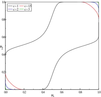
4.3.4 Distribution Level Curves
The theory in this paragraph will be the basic ingredient for simulation from Archimedean copulas. The usual way of thinking about copulas, or joint distri-bution functions in general, is: ”What is the probability that the variables of interest are jointly below certain values?”. In this subsection we will apply the reverse way of reasoning: ”Assume that we choose a certain probability level, which values for the variables correspond to that probability?”.
The level set of a bivariate copula C(u; v) for some t 2 [0;1] is given by
n
(u; v)2[0;1]2jC(u; v) =to. For a bivariate Archimedean copula that means
'¡1('(u) +'(v)) =t 12Use the fact thatf0(x) = 1
f¡10(f(x)).