AN EMPIRICAL INVESTIGATION OF PUT OPTION PRICING: A SPECIFICATION TEST OF AT-THE-MONEY OPTION IMPLIED VOLATILITY

75

AN EMPIRICAL INVESTIGATION OF PUT

OPTION PRICING: A SPECIFICATION TEST OF

AT-THE-MONEY OPTION IMPLIED VOLATILITY

Hongshik Kim

, Jong Chul Rhim

and Mohammed F. Khayum

Abstract

We statistically test the robustness of implied volatility estimates across option pricing models for at-the-money put options. The results of the specification tests show that the implied volatility estimate recovered from the Black-Scholes European option pricing model is nearly indistinguishable from the implied volatility estimate obtained from the MacMillan/Barone-Adesi and Whaley’s American put pricing model. We also investigate whether the use of Black-Scholes implied volatility estimates in American put pricing model significantly affect the prediction of American put option prices. It is shown that as long as the possibility of early exercise is carefully controlled for in the calculation of implied volatilities, predictions of American put prices are not significantly affected when the Black-Scholes implied volatility estimates are used in a specific American put option pricing model.

INTRODUCTION

Previous research has emphasized that at-the-money options are more likely to be efficient in estimating implied volatilities than away-from-the-money options [11]. Since the price of at-the-money options is more sensitive to the volatility of underlying stocks it is argued that it should provide more information about the true stock return volatility than the price of options away-from-the-money. Beckers [2] examined various weighting schemes used to calculate implied volatilities and found that the best estimates are obtained by using only at-the-money options. MacBeth and Merville [8] derived implied volatilities from the Black-Scholes European call option pricing model [3] and found that implied volatilities for out-of-the-money call options are less than implied volatilities obtained from at-the-money call options. Their results also showed that implied volatilities for in-the-money call options are greater than those for in-the-money call options. MacBeth and Merville assumed that at-the-money options are correctly priced by the Black-Scholes model and concluded that in-the-at-the-money call options are underpriced and out-of-the-money call options are overpriced. However, their conclusions are contingent upon the validity of implied volatilities recovered from the Scholes European option pricing model. Due to the Black-Scholes model’s restrictive assumptions, these estimates of implied volatilities are subject to biases resulting from various sources such as: (1) the stochastic nature of stock return volatilities, (2) misspecification of the terminal stock price distribution, and (3) the presence of early exercise possibilities.

Based on the observed linear relationship between at-the-money option prices and stock return volatilities,1 it has been shown that most of the problems mentioned above can be avoided or minimized if at-the-money options are used in estimating implied volatilities. Corrado and Miller [4] extended Feinstein’s [6,7] argument that the Black-Scholes option pricing model can recover virtually unbiased stock return volatility estimates when volatility behaves stochastically. They show that other biases, in estimating implied volatilities, resulting from misspecification of stock price dynamics can also be minimized if implied volatilities are obtained from

money options. They further show that the linear relationship between at-the-money option prices and stock return volatilities is well preserved for American options suggesting that implied volatility estimates are nearly indistinguishable across option pricing models for at-the-money options.

The purpose of this paper is to empirically test the robustness of implied volatility estimates obtained from at-the-money options using two different option pricing models. One set of volatility estimates is recovered from the Black-Scholes option pricing model and the other set of estimates is obtained from an American put valuation model developed by MacMillan [9] and Barone-Adesi and Whaley [1]. To minimize biases induced from not accounting for early exercise possibilities when recovering implied volatilities from the Black-Scholes European option pricing model, European option prices implied from observed American put prices are obtained using the put-call parity theorem [10]. We then test whether implied volatilities recovered from the Black-Scholes European model are significantly different from those derived from the MacMillan/Barone-Adesi and Whaley’s American put pricing model. Results show that these two estimates of implied volatilities are not significantly different from each other, suggesting that Corrado and Miller’s argument that implied volatility estimates are nearly indistinguishable across option pricing models for at-the-money options is correct. To further investigate whether the use of different implied volatility estimates affects pricing of American put options, theoretical prices based on the two different estimates of volatilities are compared against observed market prices. It is shown that theoretical prices based on the Black-Scholes implied volatilities fall outside observed dealers bid-ask spread boundaries slightly more than do theoretical prices based on the American model implied volatilities. However, statistical tests show that theoretical option prices based on the two different volatility estimates are not statistically different from each other. The rest of the paper outlines the estimation methodology, provides a description of the data, discusses the empirical results, and provides some concluding remarks.

ESTIMATION METHODOLOGY AND THE DATA

Implied Volatility Estimates

Implied volatilities are estimated by using Whaley’s [12] non-linear regression procedure which allows option prices to provide an implicit weighting scheme that yields an estimate of the standard deviation with minimum prediction error. Let Pj(σ) denote the theoretical price of a put option given an estimate, σ, of the stock return

volatility. The observed market price of put option is denoted by Pj. The prediction error, εj, is defined as follows:

Equation 1

εj = Pj - Pj(σ)

The estimate of σ is then determined by minimizing the sum of squared errors,

Equation 2

σ σ σ

σ

Whaley j j

j N

Min P P

= −

=

∑

* ( )

*

: ( ( ))

*

2

1

where N is the number of at-the-money option prices in each day and σ* is the estimated parameter. A numerical search routine is designed to find the optimal σ*. An initialization value is set at σ0 = 0.30, and then the equation 2

is solved iteratively using a Taylor expansion of Pj around the initialization value, σ0. Ignoring the higher-order

terms, we get:

Equation 3

Pj Pj P v

j

j

− (σ )=(σ σ− )∂ + ∂σ σ

0 1 0 0

Applying the ordinary least squares regression technique to equation 3 until |(σ1 - σ0)/σ0| < 0.0001 yields an

Using the above mentioned procedure, two types of implied volatility estimates are derived in this paper. One implied volatility estimate is recovered from a specific American option pricing model using the observed market price of American put options. Thus, the estimate of σMBAW is determined by minimizing the sum of squared errors,

Equation 4

σ σ σ

σ

MBAW jAM jMBAW j

N

Min P P

= − =

∑

where PjAM is the observed market price of American put option and PjMBAW is the theoretical price generated by the

MacMillan/Barone-Adesi and Whaley American put pricing model.

The other implied volatility estimate is derived from the Black-Scholes option pricing model using the market prices of European put option implied from the put-call parity relationship. That is, the estimate of σBS is

determined by minimizing the sum of squared errors:

Equation 5

σ σ σ

σ BS j EU j BS j N

Min P P

= − =

∑

where PjEU is the market price of European put option and PjBS is the theoretical Black-Scholes put price.

Derivation of Theoretical Prices

Implied volatility estimates obtained using the estimation technique described above are used to generate theoretical prices for an American put option based on the quadratic approximation approach developed by MacMillan [9] and Barone-Adesi and Whaley [1]. The rationale behind this approach is that, given that both American and European option prices satisfy the well-known Black-Scholes partial differential equation, it must be true that the difference in prices between an American option and an otherwise identical European option (i.e., the early exercise premium) must also satisfy the same partial differential equation. Using a quadratic approximation technique, a solution for an American put valuation formula is derived as follows:

Equation 6

PMBAW(σ*) = PBS(σ*) + A1(S/S*)q1 where S > S*, and

PMBAW(σ*) = X - S where S < S*, where:

PMBAW(σ*) denotes the MacMillan/Barone-Adesi and Whaley American put price, given the volatility estimate of σ*

PBS(σ*) denotes the Black-Scholes European put price, given the volatility estimate of σ*

A1 = -(S*/q1){1 - N[-d1(S*)]}

q1 = (1/2){-(M-1) - [(M-1)2 + 4M/K]1/2}

M = 2r/σ

K = 1 - e-r(T-t)

S* is a critical stock price which is obtained by solving the following equation: Equation 7

X - S* = PBS(S*) - {1 - N[-d1(S*)]}S*/q1

The Data

This study uses quotation data on the most heavily traded equity options on the Chicago Board of Trade Options Exchange (CBOE) from November 5 to November 30, 1990.2,3 Real time price quotation data for IBM stock options are selected from the Berkeley Options Data Base.4 An added feature is the use of a resorted format data base in this paper.5

The market price of European put options, which is not directly observable from the market, is obtained from using the call parity relationship. Assuming that options markets are efficient in the sense that European put-call parity holds, and that investors are rational in the sense that holders of American put-call options do not prematurely exercise their call options when no dividends are to be paid until option maturity, the European put-call parity equation is reconstructed by replacing a European put-call with an American put-call:

Equation 8

CA - PE = S - Xe-rT

where:

CA is the value of an American call with a striking price of X and a maturity of T, and PE is the value of a European put with a striking price of X and maturity of T.

By rearranging, we obtain the market value of a European put option:

Equation 9

PE = CA - S + Xe-rT

To impute the market value of European put options, all put-call pairs that meet the following requirements are selected.

(1) Both put and call options in a put-call pair are options on the same underlying stock, with the same strike price and the same maturity.

(2) The length of time between put and call quotes for a put-call pair must be less than 2 minutes. (3) Put and call prices are at least $1.00.6

(4) Put and call option prices within a put-call pair must satisfy the American put-call parity boundary condition.7

To isolate options on non-dividend paying stock from options on dividend paying stock, only options in a period where no dividends are paid before option maturity are selected.8 The price of options used in this study are averages of bid and ask quotes. For these time intervals during which the underlying stock price remains unchanged, the highest and lowest option prices are averaged,9 and all put-call pairs where stock prices are different, and put prices are unique, are included. After the screening process, 7,795 usable put-call pairs (daily average of 433 pairs) are identified. The average of bid and ask yield quotations on Treasury-bills that mature closest to option expiration is used to estimate a risk free rate of interest. Daily data on annualized T-bill rates are obtained from the Wall Street Journal.

HYPOTHESIS TESTING AND RESULTS

Test of Difference Between Alternative Implied Volatility Estimates

To investigate whether the two implied volatility estimates are statistically different from each other, we test the following null hypotheses that the mean value of the MBAW implied volatilities are equal to the mean value of the Black-Scholes implied volatilities:

H0: σMBAW = σBS

Rejection of the null would imply that the MBAW implied volatilities are statistically different from the Scholes implied volatilities. The results reported in Table 2 show that although the mean value of the Black-Scholes implied volatilities is slightly higher than the mean value of the MBAW implied volatilities, the two implied volatility estimates are not significantly different from each other. This finding lends support to Corrado and Miller’s [4] argument that implied volatility estimates are nearly indistinguishable across option pricing models for at-the-money options. It also suggests that option prices generated from the Black-Scholes European option pricing formula and the MBAW American option pricing model may provide the same information about future stock return volatility.

Test of Difference Between Theoretical Option Prices Based On

σσ

and

σσ

Equation 6 is used to yield two different theoretical prices, given σMBAW and σBS, respectively. Table 3 presents

the observed market price and the theoretical prices, given the two volatility estimates, for all options, for in-the-money options, for at-the-in-the-money options, and for out-of-the-in-the-money options. Both sets of theoretical prices overvalue in-the-money options and undervalue out-of-the-money options. The degree of mispricing is slightly greater for the theoretical prices based on Black-Scholes implied volatility than for those based on the MBAW implied volatility. To examine whether the two theoretical price predictions are indistinguishable from each other, we test the null hypothesis that the mean value of theoretical prices generated from using the black-Scholes implied volatility is equal to the mean value of theoretical prices based on the MBAW implied volatility. The results in Table 4 show that although the mean value ($2.85) of theoretical prices based on the Black-Scholes implied volatility is slightly greater than the mean value ($2.84) of theoretical prices based on the MBAW implied volatility, on average, both predictions are not statistically different from each other.

To further investigate whether the use of different implied volatility estimates affects pricing of American put options, theoretical prices based on the two different estimates of volatilities are compared against observed bid and ask quotes. Table 5 shows that the proportions of theoretical prices based on each of the two implied volatility estimates which falls outside dealers bid-ask spread boundaries are nearly indistinguishable (79.6% vs 79.8%) for in-the-money options. However, for out-of-the-money options the theoretical prices based on the American model fall outside the observed bid-ask spread boundaries slightly more (97.2%) than do theoretical prices based on the Black-Scholes implied volatility (94.6%). These results suggest that predictions of American put pricing are not significantly affected by the estimation of implied volatility whether the volatility estimate is recovered from the Black-Scholes European option pricing model or from a specific American put pricing model.

CONCLUSION

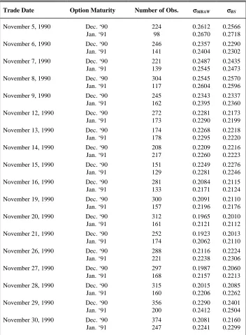
TABLE 1

Daily Implied Volatilities (σσ) Of IBM Stocks During 11/05/90 - 11/30/90*

σMBAW is implied volatility recovered from MBAW American model using market prices of American put

options.

σBS is implied volatility recovered from Black-Scholes European model using market prices of

European put options.

Trade Date Option Maturity Number of Obs. σσMBAW σσBS

November 5, 1990 Dec. ‘90 224 0.2612 0.2566

Jan. ‘91 98 0.2670 0.2718

November 6, 1990 Dec. ‘90 246 0.2357 0.2290

Jan. ‘91 141 0.2404 0.2302

November 7, 1990 Dec. ‘90 221 0.2487 0.2435

Jan. ‘91 139 0.2545 0.2473

November 8, 1990 Dec. ‘90 304 0.2545 0.2570

Jan. ‘91 117 0.2604 0.2596

November 9, 1990 Dec. ‘90 245 0.2343 0.2337

Jan. ‘91 162 0.2395 0.2360

November 12, 1990 Dec. ‘90 272 0.2281 0.2173

Jan. ‘91 173 0.2290 0.2199

November 13, 1990 Dec. ‘90 174 0.2268 0.2218

Jan. ‘91 178 0.2295 0.2220

November 14, 1990 Dec. ‘90 208 0.2209 0.2216

Jan. ‘91 217 0.2260 0.2223

November 15, 1990 Dec. ‘90 151 0.2249 0.2276

Jan. ‘91 129 0.2281 0.2246

November 16, 1990 Dec. ‘90 281 0.2084 0.2115

Jan. ‘91 133 0.2171 0.2124

November 19, 1990 Dec. ‘90 300 0.2091 0.2110

Jan. ‘91 157 0.2196 0.2176

November 20, 1990 Dec. ‘90 312 0.1965 0.2010

Jan. ‘91 161 0.2121 0.2112

November 21, 1990 Dec. ‘90 252 0.1923 0.2013

Jan. ‘91 174 0.2062 0.2110

November 26, 1990 Dec. ‘90 288 0.2116 0.2224

Jan. ‘91 221 0.2238 0.2306

November 27, 1990 Dec. ‘90 297 0.1987 0.2060

Jan. ‘91 168 0.2157 0.2213

November 28, 1990 Dec. ‘90 315 0.2015 0.2085

Jan. ‘91 160 0.2206 0.2262

November 29, 1990 Dec. ‘90 356 0.2290 0.2401

Jan. ‘91 200 0.2412 0.2504

November 30, 1990 Dec. ‘90 374 0.2081 0.2160

Jan. ‘91 247 0.2241 0.2299

*

TABLE 2

Results Of T-Tests That Mean Values Of σσMBAW and σσBS Are Equal

σMBAW is implied volatility recovered from MBAW American model using market prices of

American put options.

σBS is implied volatility recovered from Black-Scholes European model using market

prices of European put options.

T-Test σσ Type N Mean Std. Dev. t-value Prob.>|t|

H0: σMBAW = σBS σMBAW 36 0.2262 0.0188 -0.1678 0.8672

σBS 36 0.2269 0.0171

TABLE 3

Mean Values Of MBAW Theoretical Prices Of IBM Put Options: 11/05/90 - 11/30/90

P(σMBAW) is a theoretical price generated from MBAW American model given σMBAW

P(σBS) is a theoretical price generated from MBAW American model given σBS

Pobs is an observed market price of American put option

Moneyness N Pobs($) P(σσMBAW)($) P(σσBS)($)

All Options 7795 2.9610 2.8374 2.8518

In-the-Money Options 1351 5.1238 5.3427 5.3716 At-the-Money Options 2864 3.2307 3.2306 3.2617 Out-of-the-Money Options 3580 1.9289 1.5774 1.5729

σMBAWis implied volatility recovered from MBAW American model using market prices of American

put options.

σBS is implied volatility recovered from Black-Scholes European model using market prices of

European put options.

TABLE 4

Results Of T-Tests That Mean Values Of Theoretical Prices Are Equal

P(σMBAW) is a theoretical price generated from MBAW American model given σMBAW

P(σBS) is a theoretical price generated from MBAW American model given σBS

T-Test Model Price N Mean($) Std. Dev. t-value Prob.>|t|

H0: P(σMBAW) = P(σBS) P(σMBAW) 7795 2.8374 1.6545 -0.5452 0.5856

TABLE 5

Proportions Of MBAW Theoretical Prices Outside Bid-Ask Dealer Spread Boundaries

P(σMBAW) is a theoretical price generated from MBAW American model given σMBAW

P(σBS) is a theoretical price generated from MBAW American model given σBS

Pobsbid is an observed bid price of American put options

Pobsask is an observed ask price of American put options

Proportion of P(σσMBAW)

Outside Bid-Ask Boundary

Proportion of P(σσBS)

Outside Bid-Ask Boundary

Moneyness Pobsbid Pobsask N % Ave. Dev.($) N % Ave. Dev.($)

All Options 2.8972 3.0247 6056 77.7 0.1041 6365 81.7 0.0781

In-the-Money Options 5.0189 5.2288 1076 79.6 0.1625 1078 79.8 0.2021

At-the-Money Options 3.1625 3.2990 1502 52.4 0.0000 1899 66.3 0.0000

Out-of-the-Money Options 1.8843 1.9735 3478 97.2 0.3177 3388 94.6 0.3327

σMBAWis implied volatility recovered from MBAW American model using market prices of American put options.

σBS is implied volatility recovered from Black-Scholes European model using market prices of European put options.

ENDNOTES

1. For a graphical illustration, see pp. 278-280 of Cox and Rubinstein [5].

2. Among the 30 most actively traded equity options during this period, 11 to 15 options were IBM options. Daily average trading volume for IBM options exceeds 10,000 contracts.

3. November 23 data are excluded from the sample due to extremely thin trading on that day which was the Friday immediately following the Thanksgiving holiday.

4. The Berkeley Options Data Base is derived from the Market Data Report of the CBOE. The data base consists of records of bid-ask quotes and transaction data, time-stamped to the nearest second.

5. The resorted data are sorted into files, one for each trading day. Within each file, the records are sorted by ticker symbol and by chronological order.

6. Thinness in these options may result in unreasonable estimates due to the discreetness of the price change.

7. By filtering a sample based on this criterion, we avoid a joint test of market efficiency and model accuracy.

8. Since IBM stock went ex-dividend on November 5, 1990 and February 5, 1991, December and January option contracts traded during November 5 to November 30, 1990 are selected.

REFERENCES

[1] Barone-Adesi, G. and R.E. Whaley, “Efficient Analytic Approximation of American Option Values,” Journal of Finance 42, June 1987, pp. 301-320.

[2] Beckers, S., “Standard Deviations Implied in Option Prices as Predictors of Future Stock Price Volatility,” Journal

Banking and Finance 5, 1981, pp. 363-381.

[3] Black, F. and M.S. Scholes, “The Pricing of Options and Corporate Liabilities,” Journal of Political Economy 81, May/June 1973, pp. 637-659.

[4] Corrado, C. and T. Miller, “Efficient Volatility Estimates from Option-Implied Volatility,” Working Paper, University of Missouri-Columbia, 1994.

[5] Cox, J.C. and M. Rubinstein, Options Market. Englewood Cliffs, NJ: Prentice-Hall, Inc., 1985.

[6] Feinstein, S., “The Black-Scholes Formula is Nearly Linear in s for At-the-Money Options; Therefore Implied Volatilities From At-the-Money Options are Virtually Unbiased,” Working Paper, Federal Reserve Bank of Atlanta and Boston University, 1989.

[7] Feinstein, S., “The Hull and White Implied Volatility,” Working Paper, Boston University, 1992.

[8] MacBeth, J.D. and L.J. Merville, “An Empirical Examination of the Black-Scholes Call Option Pricing Model,” Journal

of Finance 34, 1979, pp. 1173-1186.

[9] MacMillan, L.W., “An Analytic Approximation for the American Put Option,” Advances in Futures and Options

Research 1, 1986, pp. 141-183.

[10] Stoll, H.R., “The Relationship Between Put and Call Option Prices,” Journal of Finance 24, 1969, pp. 801-824.

[11] Stoll, H.R. and R.E. Whaley, Futures and Options: Theory and Applications, Cincinnati, OH: South-Western Publishing Co, 1993.

[12] Whaley, R.E., “Valuation of American Call Options on Dividend-Paying Stocks: Empirical Tests,” Journal of Financial