Three-dimensional data assimilation for ionospheric reference scenarios

Three-dimensional data assimilation for ionospheric

reference scenarios

Tatjana Gerzen1, Volker Wilken1, David Minkwitz1, Mainul M. Hoque1, and Stefan Schlüter2

1_{German Aerospace Center (DLR), Institute of Communications and Navigation, Kalkhorstweg 53,}

17235 Neustrelitz, Germany

2_{European Space Agency ESA – EGNOS Project Office, 31401 Toulouse CEDEX 4, France}

Correspondence to:Tatjana Gerzen (tatjana.gerzen@dlr.de)

Received: 10 November 2016 – Revised: 3 January 2017 – Accepted: 6 January 2017 – Published: 6 February 2017

Abstract. The reliable estimation of ionospheric refraction effects is an important topic in the GNSS (Global Naviga-tion Satellite Systems) posiNaviga-tioning and navigaNaviga-tion domain, especially in safety-of-life applications. This paper describes a three-dimensional ionosphere reconstruction approach that combines three data sources with an ionospheric background model: space- and ground-based total electron content (TEC) measurements and ionosonde observations. First the back-ground model is adjusted by F2 layer characteristics, ob-tained from space-based ionospheric radio occultation (IRO) profiles and ionosonde data, and secondly the final electron density distribution is estimated by an algebraic reconstruc-tion technique.

The method described is validated by TEC measurements of independent ground-based GNSS stations, space-based TEC from the Jason 1 and 2 satellites, and ionosonde obser-vations. A significant improvement is achieved by the data assimilation, with a decrease in the residual errors by up to 98 % compared to the initial guess of the background. Fur-thermore, the results underpin the capability of space-based measurements to overcome data gaps in reconstruction areas where less GNSS ground-station infrastructure exists. Keywords. Ionosphere (mid-latitude ionosphere modelling and forecasting instruments and techniques)

1 Introduction

The ionosphere is the upper part of the atmosphere where sufficient free electrons exist to affect the propagation of radio waves. Therefore, the ionospheric parameters, such as three-dimensional electron density distribution, the

iono-spheric layer peak characteristics, and the total electron con-tent (TEC), are important information for Global Naviga-tion Satellite Systems (GNSS) users. The ingesNaviga-tion of actual ionospheric measurements into a background model, such as NeQuick (see Nava et al., 2008) or International Reference Ionosphere (IRI) (see Bilitza, 2001; Bilitza and Reinisch, 2008), is a commonly applied technique for estimating the ionospheric parameters. Several approaches had been tested for the ionospheric imaging combining actual direct and in-direct measurements with either an empirical or a physical model background (see e.g. Angling and Cannon, 2004; An-gling, 2008; Schunk et al., 2004; Wang et al., 2004; Scher-liess et al., 2009; Brunini et al., 2011; Pezzopane et al., 2011; Galkin et al., 2012; Minkwitz et al., 2015, 2016; Gerzen and Minkwitz, 2016).

Figure 1.AATR box plot for the nya2 station. Values for the disturbed period are presented in the top panel, while calm period values are in the bottom panel.

The approach presented is applied in the scope of the project DAIS (Data Assimilation Techniques for Ionospheric Reference Scenarios) to generate synthetic ionospheric refer-ence scenarios (IRSs) for the validation of the European Geo-stationary Navigation Overlay Service (EGNOS). EGNOS provides value-added services for the estimation of iono-spheric refraction effects. The IRSs are introduced by the ESA in order to conduct the EGNOS end-to-end performance simulations and to assure the integrity of the EGNOS sys-tem and associated services (see Arbesser-Rastburg, 2004; Schlüter et al., 2013).

The paper is organized as follows. At first the chosen re-construction area and periods as well as the applied database are described. Section 3 then explains the reconstruction ap-proach. Section 4 presents the validation results, and finally, the results are summarized and discussed.

2 Database and data processing

2.1 Reconstruction area and validation periods

The reconstruction approach described is tested over the ex-tended EGNOS V3 service region (−100 to 110◦_{E in} lon-gitude and−90 to 90◦_{N in latitude) with a 5 min cadence.} We select two periods in 2011, a calm period between the days of year (DOYs) 009 and 026 (9 to 26 January) and a storm period between DOY 286 and 303 (13 to 30 October). The selection of these days is based on the solar radio flux index (F10.7), the two geomagnetic indices Kp and Dst, and the along-arc total electron content rate AATRRMS1hour (see

Schlüter et al., 2013; Juan et al., 2014). The AATRRMS1hour

values are calculated at each GNSS ground-based station of the International GNSS Service used (IGS, see Sect. 2.2). The Kp and Dst indices are downloaded from the Space Physics Interactive Data Resource (SPIDR) of NOAA’s Na-tional Geophysical Data Center and the World Data Center for Geomagnetism (WDC) Kyoto. During the calm period, F10.7 was in the range of 75 to 90 solar flux units, Kp in-dex was below 4, and Dst was between−40 and 40 nT. Con-versely, the storm period reveals increased solar and geomag-netic activity, with a F10.7 of 120–170 flux units and a severe geomagnetic storm observed during the DOYs 297–298 with a Kp index above 7 and Dst values below−130 nT. Figure 1 presents as an example the AATRRMS1hour response to the

ionospheric conditions at the IGS ground-based station nya2 in Norway. The AATRRMS1hour values of each day are

or-ganized as a standard box plot. As expected, the top panel shows higher values during the disturbed period than during the calm period depicted in the bottom panel.

The impact of such conditions on the EGNOS system is given in Fig. 2. It shows the availability of the EGNOS ser-vice for aviation approaches with vertical guidance (APV-1) on DOYs 010 (left) and 298 (right) of the year 2011 (see https://egnos-user-support.essp-sas.eu/new_egnos_ops/ apv1_availability) where the EGNOS service availability on DOY 298 is crucially limited.

2.2 Ground-based GPS TEC measurements

Figure 2.The EGNOS APV-1 availability maps for DOYs 010 (left) and 298 (right) in 2011.

Table 1.IGS stations that provide independent sTEC measurements for the validation.

Station ID Country Lat. (◦N) Long. (◦E)

ohi3 Antarctica −63.3 −57.9

chpi Brazil −22.7 −45.0

mal2 Kenya −3.0 40.2

cro1 USA 17.8 −64.6

kiru Sweden 67.9 21.0

receiver network were obtained from ftp://cddis.gsfc.nasa. gov/pub/gps/data/highrate. Within the calibration procedure receiver–satellite link geometries with elevation angles less than 5◦are discarded. Thereafter, the geometry of the data is checked and only the slant TEC (sTEC) measurements with ray paths within the observed extended European area (see Sect. 2.1) are assimilated. The sTEC data of the five IGS sta-tions, listed in Table 1, are excluded from the reconstruction procedure and considered as independent references for the validation.

2.3 Ionosonde measurements

The F2 layer characteristics, in particular the critical fre-quency, foF2, and the peak height, hmF2, of 48 ionosonde stations are collected from the SPIDR database. Their cor-responding locations are depicted in Fig. 3. For validation purposes, the data of seven ionosonde stations are excluded from the reconstruction. Furthermore, the measurements of ionosonde stations JI91J and KJ609 are used both for the as-similation and the validation. All stations used for validation purposes are listed in Table 2.

In the following, the NmF2 values, calculated from the foF2 measurements by NmF2 [m−3]=1010·1.24·foF2

Figure 3.Ionosonde station positions. Black dots are ionosonde sta-tions used only for assimilation, red triangles are ionosonde stasta-tions used only for validation, and black triangles inside red triangles are ionosonde stations used for assimilation and validation.

[MHz]2, are also denoted as ionosonde measurements. In or-der to avoid artefacts in the data assimilation procedure, the ionosonde data are filtered before the application. For more details the reader is referred to Gerzen et al. (2015).

2.4 Space-based GPS TEC measurements and ionospheric radio occultation profiles

Figure 4.Reconstruction scheme.

Table 2.Ionosonde stations used for validation purposes. Ionosonde stations with italic font are used for assimilation and validation.

Station ID Country Lat. (◦N) Long. (◦E)

CS31K Australia −12.18 96.83

DB049 Belgium 50.10 4.60

HAJ45 USA 42.60 −71.50

IC437 South Korea 37.14 127.54

JI91J Peru −12.00 −76.80

JJ433 South Korea 33.50 126.53

KJ609 Republic of the Marshall Islands 9.00 167.20

MA155 Russia 55.80 37.60

TO536 Japan 35.70 139.50

2.5 TEC derived from altimeter data

Dual-frequency altimeter missions, such as Jason 1 and 2, are an excellent source for vTEC data independent of the GNSS systems. In contrast to the GNSS-derived vTEC, the altimeter measurements are naturally vertical. The available data of the Jason 1 and Jason 2 missions (http://sealevel.jpl.nasa.gov/missions/jason1/, http://sealevel. jpl.nasa.gov/missions/ostmjason2/) were downloaded from the “Open Altimeter DataBase” (http://openadb.dgfi.tum.de) and filtered for negative vTEC values and extreme outliers. These data are used for validation purposes only.

3 Scenario reconstruction approach

Figure 4 outlines a sketch of the developed assimilation pro-cess. The single steps are further detailed in the subsections of this section.

The correct characterization of the vertical shape of the profiles becomes a difficult task when assimilating only ground-based sTEC because of limited vertical information

included in these data (see e.g. McNamara et al., 2008, 2011; Minkwitz et al., 2015; Gerzen and Minkwitz, 2016). The in-clusion of space-based sTEC improves the geometry situa-tion. However, the adjustment of the background in terms of the F2 layer characteristics before starting the assimilation procedure seems to be especially advisable (e.g. Bidaine and Warnant, 2010) since the F2 layer dominates the shape of the whole profile.

Thus, we first estimate global NmF2 and hmF2 maps. For that purpose, the modified successive correction method (MSCM; see Gerzen et al., 2015) is applied. By means of MSCM, F2 layer characteristics from ionosondes and IRO profiles are assimilated into the corresponding two-dimensional background models. As global background models, the Neustrelitz Peak Density Model (NPDM; see Hoque and Jakowski, 2011) and the Neustrelitz Peak Height Model (NPHM; see Hoque and Jakowski, 2012) are de-ployed. Subsequently, the NeQuick model is adjusted by the incorporation of these maps.

The adjusted version of the NeQuick model serves as the initial guess for SMART+ (see Gerzen and Minkwitz, 2016), which is a fusion of the algebraic iterative tomogra-phy method SMART and a three-dimensional successive cor-rection method (SCM). SMART+ assimilates the ground-and space-based TEC as well as F2 layer characteristics from ionosondes and IRO profiles available over the ob-served area. SMART distributes the available integral obser-vations to the electron densities of the voxels intersected by at least one ray path, whereas the three-dimensional SCM in-troduces spatial correlation between regions covered by mea-surements and those not covered.

three-Figure 5.ReconstructedNmF2/foF2 (left) andhmF2 (right) maps.

dimensional assimilation versions within this work. Version A assimilates only ground-based sTEC and vTEC measure-ments into the NeQuick model without the precondition-ing of Step 1. Version B starts with the adjusted NeQuick (Step 1) and then includes, in addition to the ground-based TEC, space-based sTEC and F2 layer characteristics from ionosondes and IRO profiles within Step 2.

3.1 Two-dimensional assimilation by MSCM

For the assimilation of the F2 layer characteristics, MSCM is used with the same configurations as detailed in Gerzen et al. (2015). Contrary to the version used within Gerzen et al. (2015) though, both the ionosonde and IRO profile data are assimilated by MSCM here. The first estimate of the un-known parameters hmF2 or NmF2 is given by the models NPHM or NPDM respectively. Then MSCM iteratively fits the first estimate towards the measurements in the neighbour-hood.

Figure 5 presents as an example NmF2/foF2 (left) and hmF2 (right) maps reconstructed for DOY 295 in 2011 at 12:30 UT. The locations of assimilated measurements are marked magenta (dots for ionosondes and stars for IRO). The global maps are reconstructed with a 15 min cadence and are interpolated to a 5 min cadence by the linear interpolation described in Schaer et al. (1998).

3.2 Adjustment of the NeQuick model by the reconstructed F2 layer maps

To include the updated F2 layer characteristics, the inter-nal foF2 and hmF2 calculations of the NeQuick version 2.0.2 are replaced by the reconstructedfoF2/NmF2 andhmF2 maps. Moreover, the internal NeQuick model function of M(3000)F2 is replaced by the following simplified relation:

M (3000)F2= 1490

hmF2+176 (see Shimazaki 1955). In this way

the whole shape of the NeQuick electron density profiles is adjusted.

Figure 6 illustrates the possible improvement of the ad-justment described. Electron density profiles are calculated at the position of the independent ionosonde station TO536 (see Table 2) on DOY 295. The NeQuick model profile is depicted in green; the profile calculated after the inclusion of the reconstructed maps, only assimilating ionosonde ob-servations, in blue; the adjustment with ionosonde and IRO observations in red; and the measurement of the ionosonde TO536 as a violet dot.

3.3 Three-dimensional assimilation by SMART+

The TEC is related to the electron density Ne by TEC=RNe(h, λ, ϕ)ds, where s is the corresponding ray path between GNSS satellite and receiver and Ne(h, λ, ϕ)is the unknown electron density function depending on altitude

h, geographic longitudeλ, and latitudeϕ.

We discretize the ionosphere by a voxelized three-dimensional grid with a horizontal spatial resolution of 2.5◦_. The altitude resolution is 30 km for altitudes between 60 and 1000 km and increases exponentially with increasing altitude for altitudes above 1000 km. In total, 54 altitude steps are ob-tained. Assuming the electron density function to be constant within a voxel, we derive a linear system of equations (LSE):

TECs≈ n

X

i=1

Nei·asi ⇒y=Ax, (1)

wherey is the vector of the TEC measurements,xi=Nei is

the electron density in the voxeli, andasiis the length of the

ray pathsin the voxeli.

Figure 6.Electron density profiles: NeQuick model (green) and adjusted NeQuick model (blue is assimilation of ionosondes only, red is assimilation of ionosonde and IRO F2 layer data) compared with the independent ionosonde measurement (violet dot).

and the current estimate of the measurements. The electron densities of the voxels not intersected by at least one ray path remain equal to the initial guess.

In order to assimilate the F2 layer characteristics using SMART, NmF2 is expressed as TEC: for each measured NmF2–hmF2 pair the corresponding voxel numberq is cal-culated from the corresponding latitude, longitude, andhmF2 information. Then the corresponding TEC value is defined as TEC=NmF2·sq, wheresqis the length of the voxelqin the

longitudinal direction.

The iteration process stops either after a predefined num-ber of iteration steps (we used 26) or if the mean TEC devi-ation from the assimilated measurements goes below a pre-defined threshold. Thereafter, an extrapolation from the in-tersected voxels to those not inin-tersected by any TEC ray path is done using the three-dimensional SCM method, as-suming a Gaussian covariance model for the electron densi-ties (see Gerzen and Minkwitz, 2016). Figure 7 presents as an example the reconstructed electron density on DOY 295, 12:30 UT.

3.4 Calculation of the IRSs

The IRSs, i.e. vTEC maps, are calculated from the three-dimensional reconstructions by an integration of the electron density profile values using vTEC(λϕ)=

53

P

i=1

Nerec(altitudei, λ, ϕ)·(altitudei+1−altitudei). Figure 8

presents an example IRS calculated from the reconstructed electron density shown in Fig. 7.

Figure 7.Reconstructed three-dimensional electron density.

4 Validation results

4.1 Validation of the adjusted NeQuick with ionosonde characteristics

Figure 8.IRS calculated from the reconstructed three-dimensional electron density.

we derive the residuals: NmF2measured−NmF2reconstructed

andhmF2measured−hmF2reconstructedare calculated. Thereby NmF2measured and hmF2measured denote the characteristics

measured at the reference ionosonde stations (see Table 2). In Fig. 9, the distribution of the residuals over all ref-erence ionosonde stations is shown, including the mean, standard deviation (SD), and RMS of the residuals. Again, the colour green is used for the results calculated with the NeQuick model, blue for the NeQuick model assimilating solely ionosonde data, and red for the adjusted NeQuick model assimilating ionosonde and IRO data.

The residual statistics indicate the advantage of the pre-conditioning of the background using the current F2 layer characteristics. The mean of thehmF2 residuals is decreased by up to 98 % and the RMS value by up to 27 % compared to the corresponding pure NeQuick residual statistics. The NmF2 statistics are also up to 81 % lower (in relation to the magnitude). The inclusion of the IRO data in the assimila-tion procedure induces a slight addiassimila-tional improvement dur-ing the storm period. For the quiet period, no additional im-provements are visible. Therefore, one of the reasons might be inconsistencies between the ionosonde and IRO data. Dur-ing the quiet period, the deviations between the hmF2 and NmF2 values calculated by the NeQuick model and the mea-surements are comparatively small. Thus, even small incon-sistencies in the data can significantly influence the assimila-tion and validaassimila-tion results.

4.2 Validation of the IRSs with altimeter data

In this subsection we compare the absolute residuals between the Jason 1 and 2 vTEC measurements and the reconstructed vTEC derived from the reconstruction versions A and B, in detail: |vTECjason−vTECground|and|vTECjason−vTECall|

respectively. Since the Jason satellites fly at an orbit height of about 1336 km, only voxels up to this height are integrated to calculate vTECgroundand vTECall.

Jason 2 All 3.66 5.07 3.51

Quiet period Ground 3.67 4.99 3.38

Jason 1 All 7.46 11.35 8.55

Disturbed period Ground 7.82 11.26 8.10

Jason 2 All 6.96 10.64 8.04

Disturbed period Ground 7.36 10.89 8.02

In Fig. 10, the distribution of the absolute residuals is given for the two investigated periods in five TECU (total electron content unit) bins (the last bin sums up all the higher values). The vTECgroundresiduals are depicted in green, the vTECall

in red. The majority of all residuals have values less than 10 TECU.

Table 3 presents the mean, SD, and RMS values of the absolute residuals of Fig. 10. Version B decreases the mean values up to 0.4 TECU compared to version A. However, in most cases the SD of the version B residuals is higher than for version A. We assume that the partial increase in the residual deviation may be caused by inconsistencies in the assimilated ground- and space-based sTEC (see Sect. 4.3). Furthermore, there may be inconsistencies between the GPS and altimeter vTEC (see Azpilicueta and Brunini, 2009).

The histograms and statistics of the vTECground and the

vTECallresiduals are similar. Thus, to clarify the differences

between versions A and B, the ratio _|vTEC|vTECjason−vTECall| jason−vTECground| is additionally considered. This quotient is smaller than one if the additional inclusion of space-based and ionosonde data introduces an improvement. Figure 11 (quiet) and Fig. 12 (storm) present the percentage proportion between the bers of quotients that are smaller than one and the total num-ber of samples on 1 day. In other words, the numnum-ber of im-provements in percent due to inclusion of space-based and ionosonde data is shown. The green line indicates the 50 % value. The number of improved residuals is around 60 % for most of the days within the investigated periods (∼one-third higher than 60 %). The improvements are more visible dur-ing the storm period.

4.3 Validation of the three-dimensional reconstructions with ground-based sTEC

To assess the capability for estimating sTEC, the follow-ing parameters are compared: sTECmodel derived from the

initial three-dimensional electron densities calculated by the NeQuick model, sTECgroundderived from the reconstruction

version A, and sTECall from reconstruction version B are

Figure 9.Histograms ofhmF2 (top row) andNmF2 (bottom row) residuals for the periods DOYs 008–032 in 2011 (left column) and DOYs 285–306 in 2011 (right column).

Figure 10.Histogram of the vTEC absolute residuals for Jason 1 (left) and 2 (right) satellites during the quiet (top) and disturbed (bottom) periods.

stations (see Table 1). For each period the residuals between the reconstructed and the measured sTEC values are cal-culated as dTECall=sTECmeasured−sTECall, dTECground=

sTECmeasured−sTECground, and dTECmodel=sTECmeasured−

sTECmodel.

Figure 11.The percentage number of reduced absolute Jason resid-uals per day of the quiet DAIS period.

Figure 12.The percentage number of reduced absolute Jason resid-uals per day of the disturbed DAIS period.

at al. (2012) and Gerzen and Minkwitz (2016). The distribu-tions of the version A (violet) and B (red) residuals are simi-lar. Both versions crucially decrease the mean, RMS, and SD values of the residuals in comparison to the corresponding NeQuick statistics.

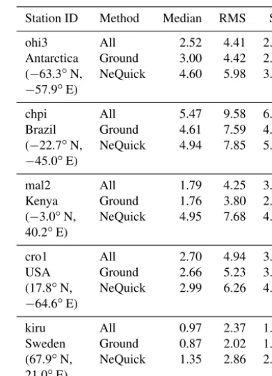
Table 4 (quiet) and Table 5 (storm) summarize the me-dian, RMS, and SD of the absolute residuals |dTECall|,

|dTECground|, and|dTECmodel| for both periods. The tables

underpin the previous histograms. Versions A and B are able to decrease the median of the residuals significantly com-pared to the initial guess of the NeQuick model. However, the inclusion of the space-based and ionosonde data in the assimilation procedure introduces no general additional de-crease in the statistics. Figure 14 indicates a possible reason for this. It depicts the scatter plots of sTECmeasured versus

sTECall(red), sTECground(violet), and sTECmodel(green) at

the reference station cro1 in the USA (17.8◦N,−64.6◦E). The measured sTEC ranges up to 140 TECU during the quiet period and up to 320 TECU during the storm period. For the quiet period, improvements from sTECmodel to sTECground

and from sTECground to sTECall are observable and are

un-derpinned by the correlation coefficients. The correspond-ing P value is around zero, indicating a high significance for the correlation coefficient. During the disturbed period, the behaviour of sTECmodel and sTECground is very

simi-lar. Conversely, for sTECall we observe that several

small-magnitude outliers of the NeQuick model (see Fig. 14, right column, third row) are removed. However, several high-magnitude outliers are simultaneously introduced (Fig. 14, right column, first row). These outliers are not visible in the sTECground figure (Fig. 14, right column, second row).

Antarctica Ground 3.00 4.42 2.66 (−63.3◦N, NeQuick 4.60 5.98 3.41 −57.9◦E)

chpi All 5.47 9.58 6.39

Brazil Ground 4.61 7.59 4.94 (−22.7◦N, NeQuick 4.94 7.85 5.02 −45.0◦E)

mal2 All 1.79 4.25 3.23

Kenya Ground 1.76 3.80 2.78

(−3.0◦N, NeQuick 4.95 7.68 4.79 40.2◦E)

cro1 All 2.70 4.94 3.37

USA Ground 2.66 5.23 3.70

(17.8◦N, NeQuick 2.99 6.26 4.54 −64.6◦E)

kiru All 0.97 2.37 1.88

Sweden Ground 0.87 2.02 1.60 (67.9◦N, NeQuick 1.35 2.86 2.12 21.0◦E)

Thus, they are most probably introduced by inconsistencies between the assimilated space-based data and the reference ground-based sTEC.

4.4 Validation summary

4.4.1 Validation with the ionosonde data

The validation of the reconstructed electron density profiles with the referenceNmF2 andhmF2 data shows a significant decrease in the evaluated statistics compared with the pure NeQuick results. The decrease is up to 98 % for thehmF2 residuals and up to 81 % for theNmF2 residuals. The inclu-sion of the IRO profile parameters in the preconditioning pro-cedure causes an additional improvement during the storm period.

4.4.2 Validation with Jason data

Figure 14.sTECmeasuredversus sTECall(top row), sTECground (middle row), and sTECmodel (bottom row) at the cro1 reference GNSS

Figure 15.Coverage of the reconstructed array by space-based data (right) and by ground-based data (left) exemplarily on DOY 011 in 2011, 09:30 UT. A pixel is coloured blue if at least one voxel above this pixel is intersected by at least one sTEC ray path.

Table 5.The statistics of the absolute sTEC residuals in TECU for DOYs 286–303.

Station ID Method Median RMS SD

ohi3 All 1.65 3.95 3.11

Antarctica Ground 1.51 3.77 3.02 (−63.3◦N, NeQuick 3.36 6.73 4.85 −57.9◦E)

chpi All 4.38 9.65 7.31

Brazil Ground 4.31 8.96 6.68

(−22.7◦N, NeQuick 5.44 10.54 7.49 −45.0◦E)

mal2 All 5.84 14.66 11.80

Kenya Ground 6.68 15.02 11.47 (−3.0◦N, NeQuick 8.65 18.80 14.16 40.2◦E)

cro1 All 9.32 23.88 18.37

USA Ground 10.09 17.49 12.03

(17.8◦N, NeQuick 10.88 18.67 12.46 −64.6◦E)

kiru All 4.35 12.93 10.45

Sweden Ground 4.33 11.94 9.31 (67.9◦N, NeQuick 11.39 24.24 17.05 21.0◦E)

4.4.3 Validation against ground-based sTEC

The assimilation of ground-based sTEC clearly improves the initial guess of the NeQuick model. The median of the TEC residuals is decreased by up to 65 % during the quiet period and by up to 62 % during the storm period. However, no or only a very small advance (up to 16 %) is observed after the additional inclusion of the space-based and ionosonde data in the assimilation procedure. This is probably due to incon-sistencies between the assimilated space-based data and the

reference ground-based sTEC as detailed in the validation section.

5 Conclusions and discussion

Within this work, time series of three-dimensional elec-tron density and IRSs, representing quiet and disturbed ionospheric conditions, are generated and cross-validated. These electron density values are deduced from the three-dimensional assimilation of ground- and space-based TEC and F2 layer characteristics into the NeQuick model.

The validation results show that a crucial improvement is achieved by the adjustment of the whole background to the measured F2 layer characteristics within a preconditioning step. A decrease in thehmF2 residual statistics of up to 98 % is hereby observed. For this preconditioning step, the IRO data are especially important due to the limited availability of ionosonde measurements, in particular over the ocean and in Africa.

Through the subsequently assimilation of the ground- and space-based TEC into the preconditioned background a de-crease of the sTEC residual statistics up to 62 % (Kiruna station) is gained. The space-based sTEC measurements cover wide regions where ground-based data are sparse (see Fig. 15). Hence, the use of additional LEO satellites (like SWARM and GRACE) looks very promising to fill the re-maining data gaps. A further advantage of the space-based data is their measurement geometry, which is complemen-tary to the angle-limited geometry of the ground-based TEC data.

variance components of parametric covariance models of the electron densities (see Minkwitz et al., 2015, 2016). How-ever, a systematic study that investigates the spatial and tem-poral electron density correlations is highly recommended.

6 Data availability

The ionosonde data, i.e. SAO files, were acquired from the following FTP server: ftp://ftp.ngdc.noaa.gov (NGDC, 2016). The IGS GNSS data were downloaded from http: //cddis.gsfc.nasa.gov (CDDIS, 2016). The data of the COS-MIC mission are available via http://www.cosmic.ucar.edu/ (UCAR, 2017) and the Jason 1 and Jason 2 altimeter data via http://openadb.dgfi.tum.de (TUM, 2017).

Competing interests. The authors declare that they have no conflict of interest.

Acknowledgements. We would like to express our gratitude to the Aeronomy and Radio Propagation Laboratory of the Abdus Salam International Centre for Theoretical Physics Trieste, Italy, providing NeQuick version 2.0.2 for scientific purposes. The au-thors thank the CDAAC (http://cdaac-www.cosmic.ucar.edu/cdaac/ rest/tarservice/data/cosmic/) for making the COSMIC data avail-able, the IGS (ftp://cddis.gsfc.nasa.gov/pub/gps/data/highrate) for making ground-based GNSS data available, the Open Altime-ter DataBase (http://openadb.dgfi.tum.de) for making the Jason data available, and the SPIDR (http://spidr.ionosonde.net/spidr/) and WDC Kyoto (http://wdc.kugi.kyoto-u.ac.jp/wdc/Sec3.html) for making ionosonde and geo-related data available.

The research presented here is partly carried out under a contract to ESA in the framework of the European GNSS Evolution Programme (EGEP).

The article processing charges for this open-access publication were covered by a Research

Centre of the Helmholtz Association.

The topical editor, K. Hosokawa, thanks L. R. Cander and the one anonymous referee for help in evaluating this paper.

TOPEX and GPS VTEC determinations, J. Geodesy, 83, 121– 127, doi:10.1007/s00190-008-0244-7, 2009.

Bidaine, B. and Warnant, R.: Assessment of the NeQuick model at mid-latitudes using GNSS TEC and ionosonde data, Adv. Space Res., 45, 1122–1128, 2010.

Bilitza, D.: International Reference Ionosphere 2000, Radio Sci., 36, 261–275, doi:10.1029/2000RS002432, 2001.

Bilitza, D. and Reinisch, B. W.: International Reference Ionosphere 2007: Improvements and new parameters, Adv. Space Res., 42, 599–609, doi:10.1016/j.asr.2007.07.048, 2008.

Brunini, C., Azpilicueta, F., Gende, M., Camilion, E., Aragn-ngel, A., Hernandez-Pajares, M., Juan, M., Sanz, J., and Salazar, D.: Ground- and space-based GPS data ingestion into the NeQuick model, J. Geodesy, 85, 931–939, doi:10.1007/s00190-011-0452-4, 2011.

CDDIS: Crustal Dynamics Data Information System (CDDIS) of the National Aeronautics and Space Administration (NASA), Receiver Independent Exchange Format (RINEX) files, available at: http://cddis.gsfc.nasa.gov, last access: 4 October 2016. Galkin, I. A., Reinisch, B., Huang, X., and Bilitza, D.:

Assimila-tion of GIRO data into a real-time IRI, Radio Sci., 47, RS0L07, doi:10.1029/2011RS004952, 2012.

Gerzen, T. and Minkwitz, D.: Simultaneous multiplicative column-normalized method (SMART) for 3-D ionosphere tomography in comparison to other algebraic methods, Ann. Geophys., 34, 97–115, doi:10.5194/angeo-34-97-2016, 2016.

Gerzen, T., Minkwitz, D., and Schlueter, S.: Comparing differ-ent assimilation techniques for the ionospheric F2 layer recon-struction, online published in J. Geophys. Res., 120, 6901–6913, doi:10.1002/2015JA021067, 2015.

Hoque, M. M. and Jakowski, N.: A new global empiricalNmF2 model for operational use in radio systems, Radio Sci., 46, RS6015, doi:10.1029/2011RS004807, 2011.

Hoque, M. M. and Jakowski, N.: A new global model for the iono-spheric F2 peak height for radio wave propagation, Ann. Geo-phys., 30, 797–809, doi:10.5194/angeo-30-797-2012, 2012. Jakowski, N., Mayer, C., Hoque, M. M., and Wilken, V.: Total

elec-tron content models and their use in ionosphere monitoring, Ra-dio Sci., 46, RS0D18, doi:10.1029/2010RS004620, 2011. Juan, J. M., Sanz, J., Rovira-García, A., González-Casado, G.,

ionosonde profiles into a global ionospheric model, Radio Sci., 46, RS2006, doi:10.1029/2010RS004457, 2011.

Minkwitz, D., van den Boogaart, K. G., Gerzen, T., and Hoque, M.: Tomography of the ionospheric electron density with geostatistical inversion, Ann. Geophys., 33, 1071–1079, doi:10.5194/angeo-33-1071-2015, 2015.

Minkwitz, D., van den Boogaart, K. G., Gerzen, T., Hoque, M., and Hernández-Pajares, M.: Ionospheric tomography by gradient-enhanced kriging with STEC measurements and ionosonde char-acteristics, Ann. Geophys., 34, 999–1010, doi:10.5194/angeo-34-999-2016, 2016.

Nava, B., Coisson, P., and Radicella, S. M.: A new version of the NeQuick ionosphere electron density model, J. Atmos. Sol.-Terr. Phy., 70, 1856, doi:10.1016/j.jastp.2008.01.015, 2008.

NGDC: National Geophysical Data Center (NGDC) of the National Oceanic and Atmospheric Administration, Ionosonde Standard Archiving Output (SAO) files, available at: ftp://ftp.ngdc.noaa. gov/, last access: 4 October 2016.

Nigussie, M., Radicella, S. M., Damtie, B., Nava, B., Yizengaw, E., and Ciraolo, L.: TEC ingestion into NeQuick 2 to model the East African equatorial ionosphere, Radio Sci., 47, RS5002, doi:10.1029/2012RS004981, 2012.

Pezzopane, M., Pietrella, M., Pignatelli, A., Zolesi, B., and Can-der, L. R.: Assimilation of autoscaled data and regional and local ionospheric models as input sources for real-time 3-D Interna-tional Reference Ionosphere modeling, Radio Sci., 46, RS5009, doi:10.1029/2011RS004697, 2011.

based data assimilation model, Radio Sci., 44, RS0A32, doi:10.1029/2008RS004068, 2009.

Schlüter, S., Prieto-Cerdeira, R., Orus-Perez, R., Lam, J. P., Juan, M., Sanz, J., and HernandezPajares, M.: Characterization and Modelling of the Ionosphere for EGNOS Development and Qual-ification. Proc. of European Navigation Conference, ENC 2013, Vienna, AT, 2013.

Schunk, R. W., Scherliess, L., Sojka, J. J., Thompson, D. C., An-derson, D. N., Codrescu, M., Minter, C., Fuller-Rowell, T. J., Heelis, R. A., Hairston, M., and Howe, B. M.: Global Assim-ilation of Ionospheric Measurements (GAIM), Radio Sci., 39, RS1S02, doi:10.1029/2002RS002794, 2004.

Shimazaki, T.: World wide daily variations in height of the maxi-mum electron density in the ionospheric F2 layer, J. Radio Res. Lab., 2, 85–97, 1955.

TUM: Technical University Munich, German Geodetic Research Institute, An Open Altimeter Database, available at: http:// openadb.dgfi.tum.de, last access: 2 February 2017.

UCAR: University Cooperation for Atmospheric Research (UCAR), COSMIC Data Analysis and Archive Center, avail-able at: http://www.cosmic.ucar.edu/data.html, last access: 2 February 2017.