An alternative way to identify local geomagnetically quiet days: a case study using wavelet analysis

www.ann-geophys.net/34/451/2016/ doi:10.5194/angeo-34-451-2016

© Author(s) 2016. CC Attribution 3.0 License.

An alternative way to identify local geomagnetically quiet days:

a case study using wavelet analysis

Virginia Klausner1,2,3, Andrés Reinaldo Rodriguez Papa3,4, Cláudia Maria Nicole Cândido2, Margarete Oliveira Domingues2, and Odim Mendes2

1_{Vale do Paraiba University – UNIVAP 12244-000, São José dos Campos, SP, Brazil} 2_{National Institute for Space Research – INPE 12227-010, São José dos Campos, SP, Brazil} 3_{National Observatory – ON 20921-400, Rio de Janeiro, RJ, Brazil}

4_{Rio de Janeiro State University – UERJ 20550-900, Rio de Janeiro, RJ, Brazil}

Correspondence to: Virginia Klausner ([email protected])

Received: 16 December 2015 – Revised: 1 March 2016 – Accepted: 4 April 2016 – Published: 19 April 2016

Abstract. This paper proposes a new method to evaluate ge-omagnetic activity based on wavelet analysis during the solar minimum activity (2007). In order to accomplish this task, a newly developed algorithm called effectiveness wavelet co-efficient (EWC) was applied. Furthermore, a comparison be-tween the 5 geomagnetically quiet days determined by the Kp-based method and by wavelet-based method was per-formed. This paper provides a new insight since the geo-magnetic activity indexes are mostly designed to quantify the extent of disturbance rather than the quietness. The re-sults suggest that the EWC can be used as an alternative tool to accurately detect quiet days, and consequently, it can also be used as an alternative to determine the Sq baseline to the current Kp-based 5 quietest days method. Another important aspect of this paper is that most of the quietest local wavelet candidate days occurred in an interval 2 days prior to the high-speed-stream-driven storm events. In other words, the EWC algorithm may potentially be used to detect the quietest magnetic activity that tends to occur just before the arrival of high-speed-stream-driven storms.

Keywords. Geomagnetism and paleomagnetism (instru-ments and techniques; general or miscellaneous) – Magne-tospheric physics (solar wind–magnetosphere interactions)

1 Introduction

A substantial part of the energy carried by the solar wind (SW) can be transferred to the terrestrial magnetosphere, and it is associated with the passage of southward-directed

inter-planetary magnetic fields past the Earth for sufficiently long intervals of time. Gonzalez et al. (1994) discussed the energy transfer process as a conversion of the mechanical energy from the SW into magnetic energy stored in the magneto-tail of Earth’s magnetosphere and its reconversion into ther-mal mechanical energy in the plasma sheet, auroral particles, ring current and Joule heating of the ionosphere.

The increase in the SW pressure is responsible for the en-ergy injections, and it induces global effects in the magneto-sphere called geomagnetic storms. The characteristic signa-ture of geomagnetic storms can be described as a depression on the horizontal component of the Earth’s magnetic field measured at low- and middle-latitude ground observatories. The decrease in the magnetic horizontal field component is due to an enhancement of the trapped magnetospheric par-ticle population as a consequence of the enhanced ring of current. This perturbation of theH component can last from several hours to several days as described by Chapman and Bartels (1940) and Sugiura (1964).

inter-planetary coronal mass ejections (ICMEs). In the CIRs and solar HSSs cases, the principal cause of geomagnetic storms is the intermittency and the brief intervals of southward mag-netic field resulting from magmag-netic field fluctuations asso-ciated with Alfvén waves (Tsurutani et al., 1995; Belcher and Davis, 1971; Tsurutani and Gonzalez, 1987; Richardson, 2006). Due to the highly oscillatory nature of the magnetic field within the CIRs, the resultant geomagnetic storms are typically only weak to moderate in intensity and the storm main phases are irregular and do not decrease smoothly with time (Tsurutani et al., 2006).

Recently, the discrete wavelet transform (DWT) has been used to classify quiescent and non-quiescent periods related to geomagnetic storms. As an alternative to the traditional Dst index (Sugiura, 1964), new indexes were developed us-ing DWT, such as the wavelet-based index of storm ac-tivity (WISA; Jach et al., 2006; Xu et al., 2008) and Wp (Nosé et al., 2012), among others. Motivated by the works of Mendes et al. (2005), Mendes da Costa et al. (2011), Hafez et al. (2013) and Klausner et al. (2014a, b, 2016a, b), which use the DWT to detect transition regions and to localize singular-ities in geophysical data, in this work, the geomagnetic varia-tion associated with the events of CIRs and HSSs in 2007 will be analyzed. To accomplish this task, the DWT will be used in three levels of decomposition to calculate the effective-ness wavelet coefficients (EWCs). With the EWCs in hand, we will be able to detect the local quiet and the local dis-turbed wavelet candidate days for each magnetic observatory chosen. The aim of this paper is to compare the 5 local quiet wavelet candidate days to the 5 quietest days determined by the German Research Center for Geosciences (GFZ) and to discuss how this selection may be used to detect the quietest magnetic activity that tends to occur before HSS events.

2 Data set

In this paper, 13 worldwide ground magnetic observato-ries distributed reasonably homogeneously have been se-lected. One of the 13 observatories chosen is Vassouras (VSS), which is located under the South Atlantic magnetic anomaly (minimum of the geomagnetic field intensity), and another four of them, Hermanus (HER), Kakioka (KAK), Honolulu (HON) and San Juan (SJG), are used to calculate the Dst index. The geomagnetic data used in this work rely on data collections provided by the International Real-time Magnetic Observatory Network (INTERMAGNET) program (http://www.intermagnet.org).

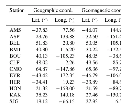
The geographic distribution of the magnetic observatories and their International Association of Geomagnetism and Aeronomy (IAGA) codes are shown in Fig. 1. Their respec-tive IAGA codes and locations are also given in Table 1. This selection of magnetic observatories is the same selec-tion used in a previous work by Klausner et al. (2013) for the same reasons (exclusion of the major influence of the auroral

Figure 1. Geographical location of the observatories used in this work and their respective IAGA code.

Table 1. INTERMAGNET network of geomagnetic observatories used in this study.

Station Geographic coord. Geomagnetic coord.

Lat. (◦) Long. (◦) Lat. (◦) Long. (◦)

AMS −37.83 77.56 −46.07 144.94

ASP −23.76 133.88 −32.50 −151.45

BEL 51.83 20.80 50.05 105.18

BMT 40.30 116.20 30.22 −172.55

BOU 40.13 −105.23 48.05 −38.67

CLF 48.02 2.26 49.56 85.72

CMO 64.87 −147.86 65.36 −97.23

EYR −43.42 172.35 −46.79 −106.06

HER −34.41 19.23 −33.89 84.68

HON 21.32 −158.00 21.59 −89.70

KAK 36.23 140.18 27.46 −150.78

SJG 18.12 −66.15 27.93 6.53

VSS −22.40 −43.65 −13.43 27.06

Source: http://wdc.kugi.kyoto-u.ac.jp/igrf/gggm/index.html (2010).

and equatorial electrojets). However, in this work, we only use the data interval corresponding to the year 2007 (solar minimum activity).

The interplanetary SW and magnetic field considered to identify the HSSs and CIRs are taken from measure-ments by the Atmospheric Composition Explorer (ACE) satellite and are available through the National Space Sci-ence Data Center (OMNIWeb): http://omniweb.gsfc.nasa. gov/form/dx1.html. The Kp and Dst indexes are extracted from the world Data Center for Geomagnetism, Kyoto (http: //wdc.kugi.kyoto-u.ac.jp).

3 Methodology

ap-−100 0 100

∆

H (nT)

0 0.5 1

d1 (nT)

0 1 2

d2 (nT)

1 2 3 4 5 6 7 8 9 10 11 12 13 14 15 16 17 18 19 20 21 22 23 24 25 26 27 28 29 30 31 0

10 20

d3 (nT)

Time (days)

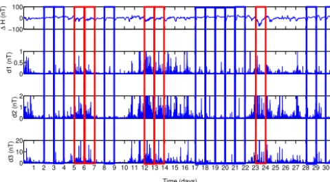
Figure 2. TheH component average variation for KAK obtained

in March 2007 is presented in the upper panel, and the square root wavelet coefficients amplitudes d1, d2 and d3, corresponding to the pseudo-periods of 3, 6 and 12 min, in the bottom three panels. The 10 geomagnetically quietest days (blue) and the 5 most disturbed days (red) are highlighted. These highlighted days are the days de-termined by the GFZ, which are deduced from the Kp index on the basis of their criteria.

plied in order to facilitate the DWT analysis visualization be-cause it has only one level of decomposition, which translates the three levels that are previously calculated by the DWT method.

Why is the DWT used in this work? The reason for us-ing the discrete wavelet methodology instead of a Fourier transform, as explained by Xu et al. (2008), is due to the geo-magnetic data containing several different kinds of variations with various spectral ranges which are related to complex current systems in the ionosphere and magnetosphere. On the one hand, the Fourier transform has been a traditional tool to analyze geophysical data. Sugiura (1964) chose a Fourier transform to identify quiet signals of expected harmonics re-lated to Earth rotation, lunar orbit and Earth orbit. Love and Rigler (2014) also performed a detailed Fourier harmonic analysis of magnetic tides using the Honolulu observatory data. On the other hand, the DWT can decompose the sig-nal into different frequency variations and obtain informa-tion localized in both frequency and space domains, while in the Fourier transform, the information is only localized in the frequency domain due to the Heisenberg principle. For these reasons, using DWT, it is possible to separate the different kinds of magnetic variations from their drivers.

3.1 Identification of local magnetic disturbance

The discrete wavelet analysis has the following property: the larger amplitudes of the wavelet coefficients are associated with locally abrupt signal changes or details of higher fre-quency. In the work of Mendes et al. (2005) and the subse-quent works of Mendes da Costa et al. (2011), Hafez et al. (2013) and Klausner et al. (2014a, 2016a), a method for the detection of the transition regions and the location of

sin-gularities due to geomagnetic events was implemented and evaluated.

In these works, the highest amplitudes of the wavelet co-efficients indicate the singularities in the geomagnetic signal in association with the disturbed periods.

In this work, we applied this methodology to the magnetic ground signal using Daubechies orthogonal wavelet function family 2 (db2). Using db2, the pseudo-periods correspond-ing to the first three wavelet decomposition levels are 3, 6 and 12 min; see Klausner et al. (2014a) for more details. These pseudo-period values are associated with our choice of wavelet function and with the data sample rate used, in this case, a 1 min time resolution.

As observed by Mendes et al. (2005) Klausner et al. (2014a, 2016a) for different observatories and magnetic storms, the periods of 3, 6 and 12 min were able to iden-tify the sudden storm commencement (SSC) and the storm main phase (SMP) in all magnetic observatory wavelet sig-natures. These magnetic field fluctuations on the ground are associated with variations in the ring current, and it is possi-ble to infer that the wavelet signatures in the first three levels are related to the ring current in this timescale range, which consequently is related to Pci 5 pulsations.

The wavelet coefficients d_kj are described as the inner product of

d_kj=

Z

f (t ) ψ_kj(t )dt, (1)

wheref (t ) is the signal withk number of points,ψ is the analyzing wavelet db2, andj is the decomposition level.

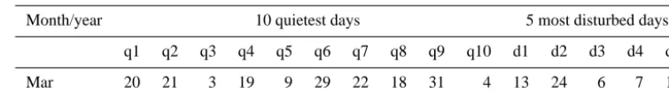
Table 2. The first 10 geomagnetically quietest days and the first 5 most disturbed days determined by the GFZ for March 2007.

Month/year 10 quietest days 5 most disturbed days

q1 q2 q3 q4 q5 q6 q7 q8 q9 q10 d1 d2 d3 d4 d5

Mar 20 21 3 19 9 29 22 18 31 4 13 24 6 7 14

Source: http://wdc.kugi.kyoto-u.ac.jp/qddays/index.html.

necessarily correspond to a non-disturbed day determined by the GFZ.

We present an example of the local magnetic disturbance identification by the DWT using three decomposition levels in Fig. 2. This figure is composed of four panels. The first panel presents geomagnetic horizontal components obtained with a resolution of 1 min at Kakioka observatory (Japan) on March 2007 and the other three present the first (d1), the second (d2) and the third (d3) wavelet decomposition level. Also, the first 10 geomagnetically quietest days are high-lighted in blue and the 5 most disturbed days in red. These days are determined by the GFZ; see Table 2. The GFZ selec-tion of the quietest days and the most disturbed days for each month is deduced from the Kp index, and it is based on three criteria for each day, such as the sum of the eight Kp values, the sum of squares of the eight Kp values and the maximum of the eight Kp values (see http://www.gfz-potsdam.de for more details). By analyzing these highlighted days in Fig. 2, we will try to validate the wavelet method as an alternative way to classify the level of geomagnetic disturbance.

In Fig. 2, the wavelet coefficients that appear simulta-neously at all three decomposition levels with amplitudes higher than the background are associated with geomagnetic storms as discussed in Mendes et al. (2005), Mendes da Costa et al. (2011), Klausner et al. (2014a) and Klausner et al. (2016a). However, we will focus on the days that present smaller wavelet coefficient amplitudes (WCAs) or that are equal to the background; i.e., these days will be the wavelet candidates for quiet days. Consequently, the days with higher amplitudes will be considered as geomagnetically disturbed. Through the analysis of WCAs, it will be possible to distin-guish the 5 quietest days from any other disturbed days in every month of 2007.

3.2 Example of the identification of magnetic disturbance and EWC

In this section, we will apply the EWC in all geomagnetic data sets in order to enhance the visualization of the wavelet coefficients. This method has been already defined in the work of Klausner et al. (2014a, 2016a, b), and it is described by the following expression:

EWC=

1 7 4

N

X

k

|d_kj=1|2+2 N

X

k

|d_kj=2|2+ N

X

k

|d_kj=3|2

!

, (2)

where the k summations are for 1 day, N=1440, consid-ering our original signals with a 1 min resolution for every month.

The EWC is weighted according to the scale decomposi-tion levels to identify the small-scale disturbances better.

One advantage of the EWC over other methods is that the EWC can be performed in times series with gaps without a need for data interpolation. In other words, a few issues such as the availability and the data quality during short periods of time and erroneous data points can be treated as gaps without compromising the analysis.

Figure 3 shows the EWC for each magnetic observatory chosen in alphabetical order as given in Table 1. Similar to Fig. 2, all these graphs have the first 10 geomagnetically quietest days and the 5 most disturbed days determined by the GFZ highlighted in blue and in red, respectively, for March 2007. The EWC also allows us to evaluate the locally quietest candidate days and the most locally disturbed candi-date days for each magnetic observatory chosen. The results of the 10 quietest and the 5 most disturbed candidate days for each observatory are presented in Table 3. In this table, the superscript letter a indicates the days where the EWC candi-date and the GFZ day are coincident and in the same order of magnetic disturbance, and superscript b indicates the days where the EWC candidate and the GFZ day are coincident but have a different order of magnetic disturbance. Compar-ing the results of candidate days with the days determined by the GFZ, we note that most of the quietest and disturbed can-didate days are classified as international quiet days (IQD) and international disturbed days (IDD), respectively, by the GFZ. The IQD and IDD vary from the highest to the lowest order of quietness and disturbance, respectively. Here, some of the candidate days correspond to the 10 IQD and/or 5 IDD but with a different order of quietness and/or disturbance.

4 Results and discussion

0 2 4 6

Kp index variation

0 2 4

EWC AMS

0 2 4

EWC ASP

0 10 20

EWC BEL

0 2 4

EWC BMT

0 2 4

EWC BOU

0 5 10

EWC CLF

0 5000 10000

EWC CMO

0 5 10

EWC EYR

0 1 2

EWC HER

0 0.5 1

EWC HON

0 1 2

EWC KAK

0 0.5 1

EWC SJG

0 1 2 3 4 5 6 7 8 9 10 11 12 13 14 15 16 17 18 19 20 21 22 23 24 25 26 27 28 29 30 31

0 2 4

EWC VSS

Time (days)

Figure 3. The effectiveness wavelet coefficients for each magnetic observatory chosen related to March 2007.

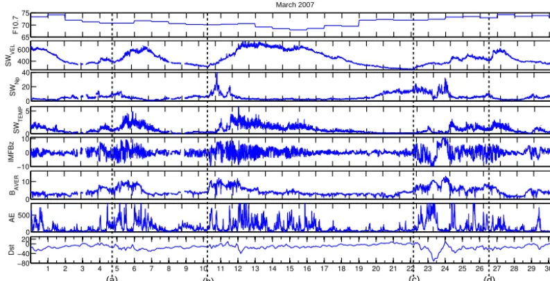
Fig. 3 and Table 3 to solar events observed in the same pe-riod. The events identified as HSSs, which mostly originated from coronal holes, are indicated in Table 4. Solar and in-terplanetary parameters associated with these HSSs events are shown in Fig. 4. In this figure, F10.7 is the solar flux (10−22Wm−2Hz−1); SWvel is the SW velocity (km s−1); SWNP is the SW density (cm3); SW temp. is the SW temper-ature (105×K); IMFBzis the interplanetary magnetic field (nT);Baveris the total magnetic field strength (nT) in GSM coordinates; AE is the auroral electrojet index (nT); and Dst is the disturbance storm time index (nT). Vertical lines indi-cate the beginning of each slow solar wind (SSW) event.

Table 4 is a slightly modified table from Xistouris et al. (2014) and it is arranged as follows: column 1 gives the stud-ied events labeled a to e; column 2 gives the date and the time of occurrence of an intensification of SW velocity; column 3

gives the date, the time and the value of the SW maximum velocity; column 4 gives the average SW velocity; and col-umn 5 gives the duration in days of the HSS.

65 70 75

F10.7

March 2007

400 600

SW

VEL

0 20 40

SW

Np

0 5

SW

TEMP

−10 0 10

IMFBz

0 10 BAVER

0 500

AE

1 2 3 4 5 6 7 8 9 10 11 12 13 14 15 16 17 18 19 20 21 22 23 24 25 26 27 28 29 30 31

−80 −40 0 20

Dst

Time (days)

(a) (b) (c) (d) (e)

Figure 4. Interplanetary parameters of March 2007. The dashed lines correspond to the starting time of the events presented in Table 4.

Table 3. The 10 geomagnetically quietest days and 5 most disturbed days obtained by the discrete wavelet analysis for March 2007.

Station 10 quietest days 5 most disturbed days

q1 q2 q3 q4 q5 q6 q7 q8 q9 q10 d1 d2 d3 d4 d5

AMS 20a 3b 9b 21b 10 29a 2 8 4b 22b 13a 15 14b 12 24b

ASP 3b 20b 21b 10 2 9b 22a 8 29b 19b 13a 15 12 14b 25

BEL 9b 20b 8 3b 22b 10 4b 21b 2 19b 13a 15 14b 12 7b

BMT 3b 10 21b 20b 9a 8 2 22b 19b 4a 13a 15 12 24b 14a

BOU 3b 20b 21b 9b 19b 10 22a 8 2 18b 13a 14b 6a 7a 12

CLF 20a 10 3a 9b 22b 8 4b 2 21b 19b 13a 15 14b 12 6b

CMO 20a 3b 21b 19a 10 4b 9b 29b 18b 22b 13a 24a 25 6b 1

EYR 3b 20b 10 2 21b 29a 9b 31b 22b 8 13a 24a 15 25 12

HER 20a 9b 8 10 3b 22b 21b 19b 2 29b 13a 25 12 6b 14a

HON 20a 10 3a 9b 8 2 21b 18a 19b 22b 13a 25 12 14b 16

KAK 3b 10 20b 9b 21b 8 2 19b 22b 4a 13a 25 12 15 24b

SJG 9b 20b 10 3b 8 19b 22a 21b 2 18b 13a 14b 25 12 6b

VSS 10 9b 8 20b 3b 19b 22a 2 21b 29b 13a 14b 12 15 25

a_{indicates the quietest and/or disturbed wavelet candidate days, with the IQD or/and IDD being coincident;}b_{indicates a wavelet candidate with a}

different order of quietness and/or disturbance from 10 IQD and/or 5 IDD.

able to estimate “the calm days before the storm” discussed by Borovsky and Steinberg (2006).

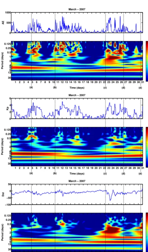
In order to show the association of HSSs and CIRs with the geomagnetic variation, we present a spectral analysis us-ing the gapped wavelet technique (GWT) of the geomagnetic indexes such as AE, Kp and Dst. The GWT can be used in the analysis of nonstationary signal to obtain information on the frequency or scale variations and to detect its struc-tures’ localization in time and/or in space (see Klausner et al. (2013) for more details). It is possible to analyze a signal in a timescale plane, the so-called wavelet scalogram that is used to provide the energy distribution in the timescale plane. In the scalograms presented in Fig. 5, areas of stronger wavelet

power are shown in dark red and the areas of low wavelet power are shown in dark blue. On thex axis the time varia-tion is plotted with a 1-day resoluvaria-tion, and the scale variavaria-tion is plotted onyaxis.

Table 4. Solar events in 2007 March.

Column 1 2 3 4 5

Event Starting time Maximum SW velocity Average SW velocity Duration

day, month, time (UT) day, month, time (UT), km s−1 km s−1 days

2007

a 5 Mar 19:00 7 Mar 13:00 628 382 3.42

b 11 Mar 06:00 13 Mar 06:00 698 299 11.29

c 23 Mar 02:00 26 Mar 07:00 498 260 4.38

d 27 Mar 12:00 28 Mar 04:00 581 425 4.04

e 31 Mar 13:00 2 Apr 20:00 645 333 7.67

0 500 1000

AE

March − 2007

Time (days)

Period (days)

1 2 3 4 5 6 7 8 9 10 11 12 13 14 15 16 17 18 19 20 21 22 23 24 25 26 27 28 29 30 31

0.125 0.25 0.5 1 2 4 5 7 9 13

30

0 2 4 5 8 10

(a) (b) (c) (d) (e)_

0 2 4 6

Kp

March − 2007

Time (days)

Period (days)

1 2 3 4 5 6 7 8 9 10 11 12 13 14 15 16 17 18 19 20 21 22 23 24 25 26 27 28 29 30 31

0.125 0.25 0.5 1

2 4 5 7 9 13

30

0 2 4 6 8 10

(a) (b) (c) (d) (e)

−100 −50 0 50

Dst

March − 2007

Time (days)

Period (days)

1 2 3 4 5 6 7 8 9 10 11 12 13 14 15 16 17 18 19 20 21 22 23 24 25 26 27 28 29 30 31

0.125 0.25 0.5 1 2 4 5 7 9 13

30

0 2 4 6 8 10

(a) (b) (c) (d) (e)_

Figure 5. Gapped wavelet spectra (bottom panel) of the geomag-netic indexes (top panel) AE, Kp and Dst for March 2007. The dashed lines correspond to the starting time of the events presented in Table 4.

wavelet spectrum analysis, the spectra of AE and Dst are well-correlated to the Kp spectrum, and consequently, they are well-correlated with the days classified as quiet and as disturbed days by the GFZ. The way that the GFZ classifies these days assumes a linear relation between magnetic obser-vatories during both quiet and disturbed times. This kind of relation to nonlinear systems, such as geomagnetic storms, can be misleading. It should be noted that even during quiet times each observatory has unequal contributions according to its local conductivity of the E-region, the local geomag-netic field intensity and its configuration, and the regional thermospheric winds (Klausner et al., 2013). However, the wavelet coefficients can detect all these nonlinear variations because each observatory magnetic data point is separately analyzed, which may be one advantage of our analysis per-formed here.

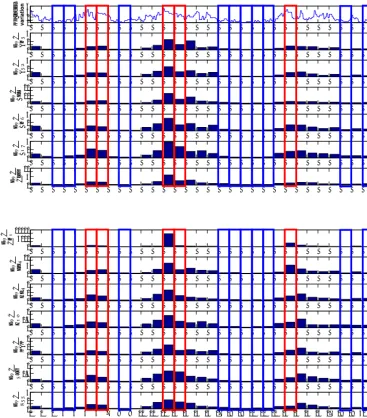
The quietest local wavelet candidate days were identified for the whole year of 2007 following the same strategy as mentioned in the context of analysis applied on March 2007. Figure 6 shows the SW velocity for the year 2007. In the upper panel, the 5 quietest days determined by the GFZ are highlighted in red. In the lower panels, the 5 quietest days for each magnetic observatory used in this work determined by the wavelet-based method are highlighted in green. The SW velocity clearly shows recurrent high-speed streams during this period. Since the Kp index varies with the SW velocity, the GFZ 5 quietest days appear mostly during the passage of low-speed SW. It can be also seen that the quietest magnetic activity tends to occur just before the arrival of high-speed SW as other researchers have previously found (Tsurutani et al., 1995; Borovsky and Steinberg, 2006). The wavelet-based method shows remarkably similar results in the detec-tion of quiet periods preceding SW HSSs to the normal Kp-based method used by the GFZ. Since the difference between these two results is rather small, it is possible to say that the wavelet-based method can be used as an alternative tool to the Kp-based method in detecting quiet SW conditions, in spite of the fact that the wavelet method is more sensitive to high-frequency magnetic variations (pseudo-periods are 3, 6 and 12 min) in comparison with Kp.

−50 0 5 5000

10000 15000

5 IQD (GFZ)

No. of obs.

IMF BZ

2000 300 400 500 600 0.5

1 1.5 2x 10

4 5 IQD (GFZ)

No. of obs.

SW (VEL)

−50 0 5

5000 10000 15000

5 IQD (Present study, CMO)

No. of obs.

IMF BZ

2000 300 400 500 600

0.5 1 1.5 2

x 104 5 IQD (Present study, CMO)

No. of obs.

SW (VEL)

−50 0 5

5000 10000 15000

5 IQD (Present study, AMS)

No. of obs.

IMF BZ

2000 300 400 500 600

1 2

x 104 5 IQD (Present study, AMS)

No. of obs.

SW (VEL)

−50 0 5

5000 10000 15000

5 IQD (Present study, EYR)

No. of obs.

IMF BZ

2000 300 400 500 600

0.5 1 1.5 2x 10

4 5 IQD (Present study, EYR)

No. of obs.

SW (VEL)

−50 0 5

5000 10000 15000

5 IQD (Present study, ASP)

No. of obs.

IMF BZ

2000 300 400 500 600

0.5 1 1.5 2

x 104 5 IQD (Present study, ASP)

No. of obs.

SW (VEL)

−50 0 5

5000 10000 15000

5 IQD (Present study, HER)

No. of obs.

IMF BZ

2000 300 400 500 600

0.5 1 1.5 2x 10

4 5 IQD (Present study, HER)

No. of obs.

SW (VEL)

−50 0 5

5000 10000 15000

5 IQD (Present study, BEL)

No. of obs.

IMF BZ

2000 300 400 500 600

0.5 1 1.5 2x 10

4 5 IQD (Present study, BEL)

No. of obs.

SW (VEL)

−50 0 5

5000 10000 15000

5 IQD (Present study, HON)

No. of obs.

IMF BZ

2000 300 400 500 600

0.5 1 1.5 2x 10

4 5 IQD (Present study, HON)

No. of obs.

SW (VEL)

−50 0 5

5000 10000 15000

5 IQD (Present study, BMT)

No. of obs.

IMF BZ

2000 300 400 500 600

0.5 1 1.5 2x 10

4 5 IQD (Present study, BMT)

No. of obs.

SW (VEL)

−50 0 5

5000 10000 15000

5 IQD (Present study, KAK)

No. of obs.

IMF BZ

2000 300 400 500 600

0.5 1 1.5 2x 10

4 5 IQD (Present study, KAK)

No. of obs.

SW (VEL)

−50 0 5

5000 10000 15000

5 IQD (Present study, BOU)

No. of obs.

IMF BZ

2000 300 400 500 600

0.5 1 1.5 2x 10

4 5 IQD (Present study, BOU)

No. of obs.

SW (VEL)

−50 0 5

5000 10000 15000

5 IQD (Present study, SJG)

No. of obs.

IMF BZ

2000 300 400 500 600

0.5 1 1.5 2x 10

4 5 IQD (Present study, SJG)

No. of obs.

SW (VEL)

−50 0 5

5000 10000 15000

5 IQD (Present study, CLF)

No. of obs.

IMF BZ

2000 300 400 500 600

0.5 1 1.5 2x 10

4 5 IQD (Present study, CLF)

No. of obs.

SW (VEL)

−50 0 5

5000 10000 15000

5 IQD (Present study, VSS)

No. of obs.

IMF BZ

2000 300 400 500 600

0.5 1 1.5 2x 10

4 5 IQD (Present study, VSS)

No. of obs.

SW (VEL)

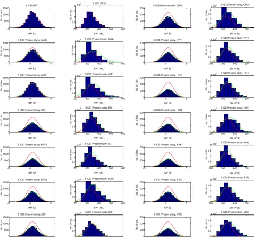
Figure 7. Distribution of IMFBzand SW velocity for the 5 quietest days determined by the GFZ and by the wavelet analysis for the 13

magnetic observatory used in this study. The histogram Gaussian distribution fit for GFZ is shown in red and, for the wavelet analysis, in green.

low-speed SW does not necessarily mean low geomagnetic activity. The coupling solar-wind–magnetosphere is most strongly controlled by the direction of the interplanetary magnetic field, being strongest when the interplanetary mag-netic field is southward (Russell, 2001). At this point, the relative contribution of the wavelet method to the identified quiet SW conditions will remain an unresolved issue.

In order to validate the 5 quietest days derived from the wavelet analysis in a more physically meaningful way, a comparison between theZ component of the interplanetary

Figure 8. Geomagnetic Sq variations at Kakioka averaged over the 5 quietest days of each month given by the GFZ definition (black lines) and (bottom) the present study (dot-dashed black lines). The 5 quietest days by the GFZ are presented in red, those by the wavelet analysis in green, and the days considered quiet by both methods in blue.

SW histogram shows the intervals between 300 and 400 km s−1_{. This behavior ofB}

zand SW is expected during quiet days. Geomagnetically quiet days are associated with near-zero or small and positive values ofBzand low SW veloci-ties (Campbell, 1989). The wavelet-based quiet days present these characteristics; therefore, these days are geomagneti-cally quiet in nature (see Fig. 7).

However, it is noticeable that the low-latitude magnetic observatories present differences between their histogram Gaussian distribution fits. This result may be explained by the fact that the Kp index is obtained as the mean value of the disturbance levels observed at 13 subauroral magnetic observatories. As discussed by Klausner et al. (2016a), the observatories located at high latitudes presented more struc-tured wavelet signatures, which are associated with rapid changes in magnetospheric and ionospheric currents in the auroral region, while at low latitudes, the wavelet signatures are smoother.

The wavelet-based method developed here could also be used as an alternative way to calculate the Sq variation us-ing quietest local wavelet candidate days. One of the many

important aspects of determining the Sq variation is to cal-culate the Dst index. The derivation of the Dst index con-sists of three main steps: the removal of the secular variation, the elimination of the Sq variation and the calculation of the hourly equatorial Dst index. The traditional method of cal-culating the Sq baseline for the quiet-day variations is to use the 5 quietest days determined by the GFZ for each month for each magnetic observatory. However, the Dst reconstruction and the quiet-time baseline remotion have been a motivation of several works (Karinen and Mursula, 2005, 2006; Mursula et al., 2008; Love and Gannon, 2009).

5 Conclusions

In this work, we implemented the wavelet-based method as an alternative way to identify local geomagnetically quiet days. This new approach addresses some issues, such as the availability and the quality of data, abrupt changes in the level of the H component, erroneous points in the database and the presence of gaps in almost all the magnetic observa-tories.

In addition, the EWC has been used to evaluate the geo-magnetically local 5 quietest days for each ground observa-tory chosen. The traditional method of calculating quiet days is using the Kp index determined by the GFZ. Our results showed that the Kp-based and the wavelet-based method present similar results. In spite of the fact that the wavelet method is more sensitive to high-frequency magnetic vari-ations, our results show that the EWC could be used as an alternative tool to the Kp-based method.

In response to the variation of SW velocity, the wavelet-based geomagnetically local 5 quietest days appear mostly during the passage of low-speed SW. This quietest mag-netic activity tends to occur just before the arrival of high-speed SW as other researchers have found (Tsurutani et al., 1995; Borovsky and Steinberg, 2006). The EWC analysis has shown great potential to detect the interval 2 calm days prior to the high-speed-stream-driven storm events.

Another important aspect of the EWC analysis is that the days determined by the wavelet-based method could be also used in other applications including the calculation of the Sq baseline. As observed for KAK, even though the 5 qui-etest days are not the same for the two cases, the average Sq-wavelet-based and Kp-based baselines are almost identi-cal.

To conclude, our methodology could be used in a semi-automatic way to characterize the quiet and disturbed mag-netic periods using a scale-time-dependent decomposition provided by the amplitude of the EWCs and filtering tech-niques. An alternative method for the detection and classifi-cation of geomagnetic signal variations may also be useful to understand the local physical processes involved in these events, and, in the near future, it could be implemented in real-time analysis. Moreover, this exploratory study encour-ages the use of alternative algorithms for Sq isolation during solar minimum activity.

Data availability

All the ground magnetic data presented in this paper can be freely downloaded using a standard internet browser from the INTERMAGNET site (www.intermagnet.org); all the in-terplanetary parameters can be obtained from the OMNIWeb (http://omniweb.gsfc.nasa.gov/form/dx1.html), and the mag-netic indexes are available from WDC Kyoto (http://wdc. kugi.kyoto-u.ac.jp).

Acknowledgements. V. Klausner wishes to thank CAPES for the financial support for her PhD (CAPES – grants 465/2008) and her postdoctoral research within the Programa Nacional de Pós-Doutorado (PNPD – CAPES) and FAPESP (grants 2011/20588-7 and 2013/06029-0). C. M. N. Cândido would like to thank CAPES, Process No. PNPD20132017-33010013008 (PNPD fellowship), for the financial support for her research. Furthermore, the authors would like to thank the GFZ, OMNIWeb, WDC Kyoto and INTER-MAGNET program for the data sets used in this work.

The topical editor, K. Hosokawa, thanks M. Herraiz and one anonymous referee for help in evaluating this paper.

References

Belcher, J. W. and Davis Jr, L.: Large-amplitude Alfvén waves in the interplanetary medium, 2, J. Geophys. Res., 76, 3534–3563, 1971.

Borovsky, J. E. and Steinberg, J. T.: The “calm before the storm” in CIR/magnetosphere interactions: Ocurrence statistic, solar wind statistic, and magnetospheric preconditioning, J. Geophys. Res., 111, A07S10, doi:10.1029/2005JA011397, 2006.

Campbell, W. H.: An introduction to quiet daily geomagnetic fields. Pure Appl. Geophys., 131, 315–331, 1989.

Chapman, S. and Bartels, J.: Geomagnetic and Related Phenomena, 1, Oxford Clarendon Press, Oxford, 1940.

Gonzalez, W. D., Joselyn, J. A., Kamide, Y., Kroehl, H. W., Ros-toker, G., Tsurutani, B. T., and Vasyliunas, V. M.: What is a geo-magnetic storm? J. Geophys. Res., 99, 5771–5792, 1994. Gonzalez, W. D., Guarnieri, F. L., Clúa de Gonzalez, A. L., Echer,

E., Alves, M. V., Ogino, T., and Tsurutani, B. T.: Magnetospheric Energetics During HILDCAAs, American Geophysical Union, 167, 175–182, 2006.

Guarnieri, F. L.: The Nature of Auroras During High-Intensity Long-Duration Continuous AE Activity (HILDCAA) Events: 1998 to 2001, American Geophysical Union, 167, 235–243, 2006.

Hafez, A. G., Ghamrya, E., Yayamab, H., and Yumotoe, K.: Un-decimated discrete wavelet transform based algorithm for extrac-tion of geomagnetic storm sudden commencement onset of high resolution records, Comput. Geosci., 51, 143–152, 2013. INTERMAGNET: International Real-time Magnetic Observatory

Network, available at: www.intermagnet.org, 2007.

Jach, A., Kokoszka, P., Sojka, L., and Zhu, L.: Wavelet-based index of magnetic storm activity, J. Geophys. Res., 111, A09215, doi:10.1029/2006JA011635, 2006.

Karinen, A. and Mursula, K.: A new reconstruction of the

Dst index for 1932–2002, Ann. Geophys., 23, 475–485,

doi:10.5194/angeo-23-475-2005, 2005.

Karinen, A. and Mursula, K.: Correcting the Dst index: Conse-quences for absolute level and correlations, J. Geophys. Res., 111, A08207, doi:10.1029/2005JA011299, 2006.

Klausner, V., Papa, A. R. R., Mendes, O., Domingues, M. O., and Frick, P.: Characteristics of solar diurnal variations: a case study based on records from the ground magnetic observatory at Vas-souras, Brazil, J. Atmos. Sol.-Terr. Phy., 92, 124–136, 2013. Klausner, V., Ojeda González, A., Domingues, M. O., Mendes, O.,

and ground magnetograms, J. Atmos. Sol.-Terr. Phy., 112, 10– 19, 2014a.

Klausner, V., Mendes, O., Domingues, M. O., Papa, A. R. R., Tyler, R. H., Frick, P., and Kherani, E. A.: Advantage of wavelet tech-nique to highlight the observed geomagnetic perturbations linked to the Chilean tsunami (2010), J. Geophys. Res.-Space, 119, 3077–3093, 2014b.

Klausner, V., Domingues, M. O. Mendes, O., Mendes da

Costa, A., and Ojeda González, A.: Latitudinal and longitu-dinal behavior of the geomagnetic field during a disturbed pe-riod: A case study using wavelet techniques, Adv. Space Res., doi:10.1016/j.asr.2016.01.018, in press, 2016a.

Klausner, V., Almeida, T., de Meneses, F. C., Kherani, E. A., Pillat, V. G., and Muella, M. T. A. H.: Chile2015: Induced mag-netic fields on the Z-component by tsunami wave propagation, Pure Appl. Geophys., doi:10.1007/s00024-016-1279-y, in press, 2016b.

Kozyra, J. U., Crowley, G., Emery, B. A., Fang, X., Maris, G., Mlynczak, M. G., Niciejewski, R. J., Palo, S. E., Paxton, L. J., Randall, C. E., Rong, P.-P., Russell III, J. M., Skinner, W., Solomon, S. C., Talaat, E. R., Wu, Q., and Yee, J. H.: Response of the Upper/Middle Atmosphere to Coronal Holes and Powerful High-Speed Solar Wind Streams in 2003, American Geophysical Union, 167, 319–340, 2006.

Love, J. J. and Gannon, J. L.: RevisedDstand the epicycles of

mag-netic disturbance: 1958–2007, Ann. Geophys., 27, 3101–3131, doi:10.5194/angeo-27-3101-2009, 2009.

Love, J. J. and Rigler, E. J.: The magnetic tides of Honolulu, Geo-physical International Journal, 197, 1335–1353, 2014.

Mendes, O. J., Domingues, M. O., Mendes da Costa, A., and Clúa de Gonzalez, A. L.: Wavelet analysis applied to magnetograms: Singularity detections related to geomagnetic storms, J. Atmos. Sol.-Terr. Phy., 67, 1827–1836, 2005.

Mendes da Costa, A., Domingues, M. O., Mendes, O., and Brum, C. G. M.: Interplanetary medium condition effects in the south at-lantic magnetic anomaly: A case study, J. Atmos. Sol.-Terr. Phy., 73, 1478–1491, 2011.

Mursula, K., Holappa, L., and Karinen, A.: Correct normalization of the Dst index, Astrophysics and Space Sciences Transactions, 4, 41–45, 2008.

Nosé, M., Iyemori, T., Wang, L., Hitchman, A., Matzka, J., Feller, M., Egdorf, S., Gilder, S., Kumasaka, N., Koga, K., Mat-sumoto, H., Koshiishi, H., Cifuentes-Nava, G., Curto, J. J., Segarra, A., and Celik, C.: Wp index: A new substorm index de-rived from high-resolution geomagnetic field data at low latitude, Space Weather, 10, S08002, doi:10.1029/2012SW000785, 2012. OMNIWeb: Interface to produce plots, listings or output files from OMNI 2, available at: http://omniweb.gsfc.nasa.gov/form/dx1. html, 2007.

Richardson, I. G., Cliver, E. W., and Cane, H. V.: Sources of ge-omagnetic activity over the solar cycle: Relative importance of coronal mass ejections, high-speed streams, and slow solar wind, J. Geophys. Res.-Space, 105, 18203–18213, 2000.

Richardson, I. G.: The Formation of CIRs at Stream-Stream Inter-faces and Resultant Geomagnetic Activity, Geoph. Monog. Se-ries, 167, 45–58, 2006.

Russell, C. T.: Solar Wind and Interplanetary Magnetic Field: A Tutorial, in: Space Weather, edited by: Song, P., Singer„ H. J., and Siscoe, G. L., American Geophysical Union, Washington, DC, doi:10.1029/GM125p0073, 2001.

Smith, E. J. and Wolfe, J. H.: Observations of interaction regions and corotating shocks between one and five AU: Pioneers 10 and 11, Geophys. Res. Lett., 3, 137–140, 1976.

Sugiura, M.: Hourly values of equatorial Dst for the IGY, Annals of the International Geophysical Year 35, 9, 9–45, Pergamon Press, Oxford, 1964.

Tsurutani, B. T. and Gonzalez, W. D.: The cause of high-intensity long-duration continuous AE activity (HILDCAAs): Interplane-tary Alfvén wave trains, Planet. Space Sci., 35, 405–412, 1987. Tsurutani, B. T., Gonzalez, W. D., Clúa de Gonzalez, A. L., Tang, F.,

Arballo, J. K, and Okada, M.: Interplanetary origin of geomag-netic activity in the declining phase of the solar cycle, J. Geo-phys. Res., 100, 21717–21733, 1995.

Tsurutani, B. T., Gonzalez, W. D., Clúa de Gonzalez, A. L., Guarnieri, F. L., Gopalswamy, N., Grande, M., Kamide, Y., Kasa-hara, Y., Lu, G., Mann, I., McPherron, R., Soraas, F., and Va-syliunas, V.: Corotating solar wind streams and recurrent ge-omagnetic activity: A review, J. Geophys. Res., 111, A07S01, doi:10.1029/2005JA011273, 2006.

Turner, N. E., Mitchell, E. J., Knipp, D. J., and Emery, B. A.: En-ergetics of Magnetic Storms Driven by Corotating Interaction Regions: A Study of Geoeffectiveness, in Recurrent Magnetic Storms: Corotating Solar Wind Streams, American Geophysical Union, 167, 113–124, 2006.

WDC Kyoto: World Data Center for Geomagnetism, Kyoto, avail-able at: http://wdc.kugi.kyoto-u.ac.jp, 2007.

Xistouris, G., Sigala, E., and Mavromichalaki, H.: A complete Cat-alogue of High Speed Solar Wind Streams during Solar Cycle 23, Solar Physics, 289, 995–1012, 2014.