www.ann-geophys.net/34/55/2016/ doi:10.5194/angeo-34-55-2016
© Author(s) 2016. CC Attribution 3.0 License.
Mapping of steady-state electric fields and convective drifts in
geomagnetic fields – Part 1: Elementary models
A. D. M. Walker1and G. J. Sofko2
1School of Chemistry and Physics, University of KwaZulu-Natal, Durban, South Africa
2Institute of Space and Atmospheric Studies, University of Saskatchewan, Saskatchewan, Canada Correspondence to: A. D. M. Walker ([email protected])
Received: 26 October 2015 – Revised: 13 December 2015 – Accepted: 17 December 2015 – Published: 19 January 2016
Abstract. When studying magnetospheric convection, it is often necessary to map the steady-state electric field, mea-sured at some point on a magnetic field line, to a magneti-cally conjugate point in the other hemisphere, or the equa-torial plane, or at the position of a satellite. Such mapping is relatively easy in a dipole field although the appropriate formulae are not easily accessible. They are derived and re-viewed here with some examples. It is not possible to derive such formulae in more realistic geomagnetic field models. A new method is described in this paper for accurate map-ping of electric fields along field lines, which can be used for any field model in which the magnetic field and its spa-tial derivatives can be computed. From the spaspa-tial derivatives of the magnetic field three first order differential equations are derived for the components of the normalized element of separation of two closely spaced field lines. These can be in-tegrated along with the magnetic field tracing equations and Faraday’s law used to obtain the electric field as a function of distance measured along the magnetic field line. The method is tested in a simple model consisting of a dipole field plus a magnetotail model. The method is shown to be accurate, con-venient, and suitable for use with more realistic geomagnetic field models.
Keywords. Ionosphere (ionosphere-magnetosphere interac-tions; instruments and techniques) – magnetospheric physics (instruments and techniques)
1 Introduction
In studies of magnetospheric convection, such as those by the SuperDARN network (Greenwald et al., 1995), the map-ping of electric fields along magnetic field lines to the
lo-cation of satellites on the same field line or the conjugate point in the ionosphere in the opposite hemisphere is of con-siderable importance. Except in the neighbourhood of strong auroral activity it can be assumed that the parallel conduc-tivity is infinite so that for large-scale electric fields that are electrostatic on the timescale of interest, the magnetic field lines are equipotentials. For a dipole magnetic field, the map-ping is easy, although, surprisingly, techniques for doing so are not explicitly covered in elementary texts on sphere physics. For more realistic models of the magneto-sphere where the magnetic field lines are stretched, as they are for lines reaching the magnetic equator at distancesr0 beyond geostationary orbit, the problem of mapping can be-come quite complex.
Most mapping has been done by concentrating on the elec-tric potential. For an electrostatic field the magnetic field lines are equipotentials. If the field is required several mag-netic field lines are traced and their separation calculated. From their separation the gradient of the electric potential is estimated to give the electric field. Examples of this approach are in Lyons and Williams (1984, chapter 2) for a dipole field and Baker et al. (2004) for a more general field. This is in-herently inaccurate, requiring the evaluation of a small dif-ference of large quantities. For example, the typical length of an auroral latitude field line is 105km. If we compare electric fields at the conjugate points in the ionosphere by consider-ing two field lines separated by 10 km at the ground, then in order to achieve 10 % accuracy (1 km) in the field line sep-aration at the conjugate point the arrival points of the two adjacent field lines must be computed to 1 part in 105.
deriva-tives are given at all points of interest. Provided that the mag-netosphere is in a steady state, the electric field mapping is a straightforward application of Faraday’s law. If the element of separation of two field lines can be calculated as a func-tion of posifunc-tion on the field line, then, since the field lines are equipotentials, the electric field can be calculated. Since the separation is calculated by integrating an analytic formula along with the field line, its accuracy is the same as that of the field line position.
It is, however, also very useful to have as a reference the expected mapping for a purely dipole field. The derivation of expressions for mapping in a dipole field is straightforward, but, surprisingly, no convenient collection of the relevant mulae seems to be available. Mozer (1970) has provided for-mulae for the special case of mapping the ionospheric elec-tric field to the dipole equatorial plane but not the more gen-eral formulae. There appears to be no simple published ver-sion of the actual mapping of the components ofEand of the components of the convective drift between conjugate points along dipole field lines.
We therefore first provide an easily accessible derivation of a number of relevant formulae for a dipole field. They are useful for tutorial purposes and provide analytic expressions for validating the new tensor field mapping techniques. These mappings are used for some illustrative examples which give rough estimates of how electric fields and convective drifts vary with altitude. For example, we make comparisons be-tween convective drifts measured by the DMSP satellites at about 840 km altitude and SuperDARN F-region measure-ments in the 250–325 km altitude range, forLvalues of about 6.6 and lower. For L∼6.6, these comparisons should nor-mally show that the DMSP measurements should be about 14 % greater, simply because of the mapping of the convec-tive drift from the F-region to DMSP altitude.
Finally we introduce a new method in which a second rank tensor is analytically derived which satisfies a set of first or-der differential equations. This tensor provides a measure of the divergence and convergence of the field lines and can be found by a step-by-step integration of the differential equa-tions simultaneously with the tracing of the magnetic field line. This can be used to deduce the electric field without the inaccuracies inherent in the method used, inter alia, by Baker et al. (2004). The method is tested for a simple model con-sisting of a dipole field with a Harris (1962) current sheet to simulate the magnetotail.
2 Mapping in a dipole field 2.1 Basic ideas
All mapping techniques depend on the same principle. Ex-cept where there are electric fields parallel toB, for example near auroral arcs, the magnetic field lines are equipotentials.
We may write Faraday’s law in the form I
E·dl=0 (1)
provided that the timescales on which changes take place is longer than the Alfvén transit time so that the magnetic in-duction d8/dtcan be ignored. If we then consider a contour bounded by two adjacent field lines and terminated at each end by line segmentsδwnormal toBthen there is no contri-bution to the integral from the portion of the contour coincid-ing with the field lines. Then ifE1is the component of the electric field parallel tow1andE2that parallel tow2, (Eq. 1) becomes
E1δw1−E2δw2=0 (2) or
E1 E2 =
δw2
δw1. (3)
Thus we simply need to find how δw changes along the field lines and the electric field component along it is in-versely proportional to its magnitude. Equivalently, the mag-netic field lines lie on electric equipotentials so that the elec-tric field is perpendicular to the magnetic field. If we consider two closely spaced magnetic field lines separated by perpen-dicular distanceδw and having an electric potential differ-enceδ8then the component of the electric field parallel to δwis given by
E= − lim δw→0
δ8 δw ∝
1
δw. (4)
Mozer (1970) gives expressions for the mapping of the electric field between the ionosphere and the equatorial plane:
EMi
EMe = 2L r
L−3
4 (5)
EWi
EWe = L
3/2, (6)
whereEM is the component of the electric field perpendicu-lar toBin the meridian plane andEWis the westward com-ponent. The subscriptsianderefer to the values at the iono-sphere and the equatorial plane, although actually the formu-lae are calculated as if the ionosphere was at zero altitude. We shall generalize these to apply to the mapping between any two points on a magnetic field line.
2.2 Dipole field geometry
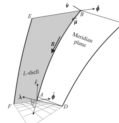
Earth is shown in Fig. 1. We can use a spherical polar system with the axis coincident with the dipole axis. Rather than po-lar angle we use its complement, the magnetic latitude. This is not the same as the magnetic latitude defined in realistic models of the magnetic field.
The field is given as a function of position by
B=BeqR
3 E r3
n
−2rˆsinλ+ ˆλcosλ o
, (7)
where the unit vectors are along the radial and latitudinal di-rections,Beqis the field at the surface of the earth at the equa-tor (∼3.154×10⁻⁵T),REis the Earth’s radius (∼6378 km), λis the magnetic latitude, and ris the radial distance from the Earth’s centre.
The equation of a dipole field line is
r=RELcos2λ, (8)
whereLis the radial distance at which the field line crosses the equator, measured in Earth radii. The radius r can be eliminated from Eqs. (7) and (8) to giveBas a function ofλ on the field line defined by the parameterL:
B=
B0 n
−2rˆsinλ+ ˆλcosλo
cos6λ , (9)
whereB0, the value ofBat the apex of the field line is
B0=Beq/L3. (10)
The magnitude of the magnetic field as a function of latitude on the field line is then
B=B0
p
1+3sin2λ
cos6λ . (11)
The magnetic field lines lie in the magnetic meridian plane, in which the unit vector parallel to the magnetic field is given by
ˆ
µ=−2rˆsinλ+ ˆλcosλ
p
1+3sin2λ
. (12)
The unit outward normal vector in the meridian plane is given by
ˆ
ν=rˆcosλ+2 ˆ λsinλ p
1+3sin2λ
. (13)
We complete the right-handed system with a unit vector
ˆ
φ normal to the meridian plane in the easterly direction. The right-handed coordinate system is defined by the vec-torsµˆ,νˆ,φˆ, in that order. This system of local coordinates is easily generalized to situations where the field lines do not lie in a plane. The directions of the unit vectors are shown
B
r^ L-shell
Me ridian
plane
A
B
C
D E
F
^
^ ^
[image:3.612.325.527.65.274.2]^
Figure 1. Dipole field: directions of unit vectors.
in Fig. 1. The grid at the bottom of the figure shows lines of latitude and longitude at the Earth’s surface.
The figure also shows the unit vectorsrˆin the radial direc-tion andλˆ in the direction of increasing latitude. The angle betweenλˆ andµˆ is the dip angleψ, as is the angle between
ˆ
randνˆ. Thus
cosψ= ˆλ· ˆµ= ˆr· ˆν (14)
and from Eqs. (12) or (13) cosψ= cosλ
p
1+3sin2λ
. (15)
The element of perpendicular distance between two field lines that lie in the meridian plane is
δwν=δrcosψ. (16)
The elementδris the radial length element at constantλso that, from (Eq. 8),
δr=
∂r
∂L
λ
δL=REcos2λδL. (17) Thus
δwν=
REcos3λ p
1+3sin2λ
δL. (18)
Sometimes we need to consider a horizontal path between the field linesLandL+δL. At a fixed radiusrEq. (8) for a field line can be differentiated, keepingrconstant, to obtain 0=REcos2λ δL−2RELsinλcosλ δλ (20) so that, at any fixed radiusrand latitudeλ, the change inL in moving to a neighbouring field line atλ+δλis
δL=2Ltanλ δλ. (21)
If we assume that there are no potential drops along the magnetic field lines, then there can be no component of the electric field parallel to the magnetic field, and therefore can only have components alongνˆandφˆ, so we can write
E= ˆνEν+ ˆφEφ. (22)
SinceνˆEν= ˆrEr+ ˆλEλ, from Eq. (13) we get
Er =
cosλ p
1+3sin2λ
Eν (23)
Eλ = 2 sinλ
p
1+3sin2λ
Eν (24)
and thusEr andEλare related by
Er =1
2Eλcotλ. (25)
The mapping of the perpendicular components of the elec-tric field is now straightforward. We specify a point on the field line by its latitude λ. Then from the general mapping relation (Eq. 2) and the expression (Eq. 18) the ratio between the ν-components of the electric field at two different lati-tudes is
Eν1 Eν2 =
cos3λ2 cos3λ1
s
1+3sin2λ1 1+3sin2λ2
(26)
and from Eq. (19) that between theφcomponents is Eφ1
Eφ2
=cos
3λ2 cos3λ
1
. (27)
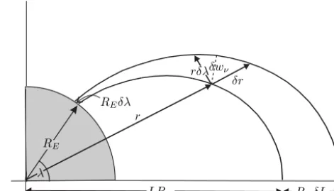
[image:4.612.311.547.68.203.2]There are two closed paths we shall use for Eq. (1). First, we integrate in the meridian plane between an ionospheric segment at a fixed altituder=constant, then along the field line labelledL(whereLREis the radial distance at which the line reaches the equator), then radially outward from LRE to (L+δL)RE and finally back along the field line to the ionosphere, as shown in Fig. 2. Then (Eq. 1) becomes Eλr δλ=Er,eqREδL. (28)
Figure 2. Dipole field: meridian plane.
Then Eqs. (8), (21), and (28) can be used to show that
Er,0= cos
3λ
2 sinλEλ, (29)
where the subscript 0 refers to the value at the apex of the field line.
We can eliminateEλfrom Eq. (24) and (29) to obtainEν in terms ofEr,0
Eν = p
1+3sin2λ
cos3λ Er,0. (30)
The total field can then be written
E=rˆcosλEr,0+2 ˆ
λsinλEr,0+ ˆφEφ,0
cos3λ . (31)
2.3 Mapping the convective drift The convective or Hall drift is given by
vH=
E×B
B2 =
ˆ
νEφ− ˆφEν
B , (32)
which gives the convective (Hall) drift in terms of the two E-vector components perpendicular to B. From Eqs. (30) and (27) this becomes
vH=
ˆ
νEφ,0cos3λ B0p1+3sin2λ
ˆ
φEr,0cos3λ B0
. (33)
We can take the cross product ofEandBgiven by Eqs. (7) and (31) to express the drift in spherical polar coordinates
vH = rˆEφ,0cos
4λ B0(1+3sin2θ )
+2 ˆ
λEφ,0sinλcos3λ B0(1+3sin2λ)
ˆ
φEr,0cos3λ B0
. (34)
and(r2, λ2). From Eq. (33), the meridian plane convective velocity component ratio is
vν,2 vν,1
= cos
3λ 2 cos3λ
1 s
1+3sin2λ1 1+3sin2λ2
=
r 2 r1
3/2s4L−3r 1/RE 4L−3r2/RE
(35) and the eastward velocity component ratio is
vφ,2 vφ,1
=cos
3λ 2 cos3λ
1
=
r 2 r1
3/2
. (36)
Consider as an example the mapping from the ionosphere to a DMSP satellite. Table 1 gives the ratios of the velocity components for mapping along field lines of varyingLfrom an ionospheric heighth1to DMSP at an assumed altitudeh2 of 840 km, usingRE=6378 km.
2.4 Cross-section of a magnetic flux tube
Sinceνˆ andφˆ are mutually perpendicular, and both are nor-mal toB, the element of cross-sectional area of a flux tube is
δA= ˆνδwν× ˆφδwφ= ˆµδwνδwφ (37) We use Eqs. (18) and (19) to show that
δA= LR
2 Ecos6λ p
1+3sin2λ
δLδφ (38)
so that, using Eq. (11)
BδA=BeqRE2LδφδL=B0δA0 (39) expressing the conservation of magnetic flux along a field line. This is, of course, merely a verification that our deriva-tion of the quantities δwν andδwφ is correct. However, in what follows, when the magnetic field is not dipolar, the com-parison of the computed cross-sectional area with the mag-netic field is a valuable method of checking the accuracy of the method of computation.
3 Field mapping in general models of the magnetic field Mathematical models of the geomagnetic field are now avail-able that not only provide for a good fit to the Earth’s interior field, but also allow for the various exterior current systems arising from the interaction of the solar wind and the mag-netosphere. The IGRF is a spherical harmonic representation of the interior field (Maus et al., 2005) while Tsyganenko (1987, 1995, 1996) has used solar wind data to determine ap-propriate parameters for the exterior field model where each contribution is given by appropriate polynomials of the co-ordinate system with the coefficients determined by the solar
wind conditions. In such a model the magnetic field is speci-fied everywhere as a function of position
B=B(r), (40)
whereris the position.
We discuss the mapping of electric fields along field lines in such a model. It is not the intention of this paper to perform detailed calculations in the various realistic models; this will be left to a future paper. We discuss only the principles with illustrative calculations in a simplified model.
In what follows we use vector notation and Cartesian ten-sor notation (eg Walker, 2005, Appendix A1) interchange-ably as convenient. A subscriptitakes the values (1,2,3) rep-resenting the three Cartesian components of a vector. Second rank Cartesian tensors have two subscripts. A repeated suf-fix implies summation. Consider a field line originating at a point located at a radiusri. An adjacent point on the field line is atri+δri where the magnitude ofδri isδs. The notation is that differencesδrepresent the difference between quanti-ties measured on the adjacent field lines, while differences1 arise as a consequence of moving along the field line.
The unit vector parallel to the field line is dri(s)
ds ≡ ˆµi= Bi
B. (41)
If the magnetic field is defined throughout space this is a set of three first order simultaneous differential equations for the field line. They can be integrated numerically step by step using a Runge-Kutta or other suitable process.
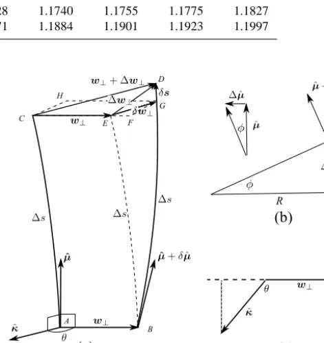
Now consider a field line passing through some point in space that is taken as the origin as shown in Fig. 3a. At a point A, distancesalong the field line, the unit vectorµˆ ≡B/Bis directed parallel to the field line. An adjacent field line passes through pointB, displaced, normal toµˆ, by a small amount w⊥i . The adjacent field line lies alongBD. Taylor’s theorem shows that, to first order inwi⊥, the unit vector tangent to the second field line atBis
ˆ
µi+δµˆi= ˆµi+ ∂µˆi
∂xjw
⊥
j = ˆµi+Tijw⊥j, (42) where
Tij≡ ∂µˆi ∂xj
. (43)
Note that unit vectors can only change direction not mag-nitude. Since µiˆ is a unit vector, δµiˆ is normal to it, and has components parallel and perpendicular tow⊥i . The par-allel component arises from the divergence of the two field lines while the perpendicular component is the consequence of shear of the field lines.
If we now advance a small distance1s fromAtoC and fromBtoDthe separation of the adjacent field line iswi⊥+
Table 1. Mapping of the convective drift from the ionosphere at heighth1to DMSP altitudeh2=840 km along dipole field lines of varying L. The ratio of the eastward (φ) components (column 2) does not change withL. The ratio of velocity componentsvν in the magnetic meridian plane is given for variousL.
h1 vφ,2/vφ,1 vν,2/vν,1 vν,2/vν,1 vν,2/vν,1 vν,2/vν,1 vν,2/vν,1 vν,2/vν,1 vν,2/vν,1 (km) (allL) L=6.6 L=6.0 L=5.5 L=5.0 L=4.5 L=4.0 L=3.0
350 1.1112 1.1168 1.1174 1.1181 1.1189 1.1199 1.1213 1.1260 300 1.1237 1.1299 1.1306 1.1314 1.1323 1.1334 1.1350 1.1402 250 1.1365 1.1433 1.1441 1.1449 1.1459 1.1472 1.1489 1.1546 200 1.1494 1.1569 1.1578 1.1587 1.1598 1.1612 1.1631 1.1694 150 1.1627 1.1708 1.1718 1.1728 1.1740 1.1755 1.1775 1.1827 100 1.1762 1.1850 1.1860 1.1871 1.1884 1.1901 1.1923 1.1997
1s. The distance BG is also of length 1s. If we were to move from pointBa distance1sin a straight line along the direction of µˆ we would reach the pointE while along the direction of µˆ +δµˆ we would reachG. The displacement from E toG is δw⊥ and results from the divergence and
shear of the field lines. Clearly, since the magnitude ofµˆ is unity,
δwi⊥ 1s =
δµˆi
1 =Tijw
⊥
j . (44)
The vectorw⊥+δw⊥is not, however, perpendicular to the
field line atCbecause of the curvature. It must be rotated to pointDto coincide withw⊥+1w⊥. The definition of the
field line curvature is illustrated in Fig. 3b (Walker, 2005, Appendix B.2). A small arc of length 1s on the field line subtends an angleφat the centre of curvature. The unit vector
ˆ
µi, tangent to the field line rotates along the arc through the same angleφ. In the limitφ→0,1µˆi is normal toµˆi. The curvatureκ is defined as a vector of magnitude 1/Rdirected towards the centre of curvature. Clearly, in the limit of small φ,
φ=1µˆ
1 =
1s
R (45)
so that
κ =dµˆ
ds =(µˆ.∇)µˆ ⇒ ˆµjTij. (46) As shown in Fig. 3cκ makes an angleθwithw⊥. The
com-ponent ofw⊥alongκis the scalar product ofw⊥and the unit
vectorκˆ. It is positive whenθis an acute angle and negative when it is obtuse. The vectorδsis then given by
δs ˆ κ.w⊥
= − ˆµ1s
R (47)
or, in subscript notation δsi
1s = − ˆµi
ˆ
κjw⊥j
R = − ˆµiκjw
⊥
j = − ˆµiµkTj kˆ w
⊥
j. (48)
Figure 3. Definition ofTij. (a) Relative displacement of adjacent
field lines; (b) Field line curvature; (c) Component ofw⊥ along
curvature vector.
The elements ofTijare given by Tij =
∂µiˆ
∂xj = ∂ ∂xj
Bi
B
= 1
B
∂Bi ∂xj −
Bi B
∂B ∂xj
= 1
B
δik−BiBk
B2 ∂B
k ∂xj
(49) and the components of B and its derivatives may be found from the model. Finally
1w⊥i =δw⊥i +δsi (50) so that, from Eqs. (44) and (48)
dw⊥i ds =Tijw
⊥
[image:6.612.310.546.185.435.2]Figure 4. Covariant and contravariant components ofE.
of the electric field. To map a component of the electric field along a field line, Eqs. (41) and (51) can be integrated nu-merically to the desired end point. The mapping procedure is then as follows:
– The initial value for integrating (Eq. 51) is a unit vector in the direction of the desired component of the electric fieldE.
– Equations (41) and (51) are integrated step by step along the field line giving the coordinates of the field line and the coordinates of the vectorw⊥as a function of
dis-tancesalong the field line.
– The mapped electric field component in the direction of w⊥ at each point on the field line has magnitude
E0/w⊥.
– The procedure can be carried out for two initial values ofw⊥to give two components of the field line.
Although the two initial values ofw⊥may be at right
an-gles to each other, there is no reason to suppose that they will remain at right angles as the integration proceeds along the field line. The computation of the resultant electric field therefore requires care. In general, the directions of the two values ofw⊥define a set of two-dimensional oblique
coordi-nates as shown in Fig. 4. The two components ofEthat have been calculated areE1andE2, the covariant components in the oblique system. To calculate the resultantEwe need the contravariant components given by
E1 = E1−E2cosθ
sin2θ (52)
E2 = −E1cosθ+E2
sin2θ , (53)
as can be seen from the figure. The resultantEis calculated from these using the parallelogram rule.
4 A simple night-side model 4.1 Characteristics of the model
We illustrate the use of the first order differential Eqs. (41) and (51). We use a right-handed CGM coordinate system with origin at the centre of the Earth,x directed towards the Sun,y from dawn to dusk andznorthward along the axis. The magnetic field is a dipole field with the addition of a Harris (1962) current sheet to represent the tail. The mag-netic field components are then given by
Bx = −
3BeqR3Exz
(x2+y2+z2)5/2+Bhtanh z
d (54)
By = − 3BeqR
3 Eyz
(x2+y2+z2)5/2 (55) Bz = BeqR
3
E(x2+y2−2z2)
(x2+y2+z2)5/2 , (56) where the last term in Eq. (54) arises from a Harris cross tail current. This model is not over-complicated and gives qualitatively realistic magnetic fields on the night side.
The derivatives of the components of B are then ∂Bx
∂x =
3BeqRE3z(4x2−y2−z2)
(x2+y2+z2)7/2 (57) ∂Bx
∂y =
15BeqRE3xyz
(x2+y2+z2)7/2 (58) ∂Bx
∂z =
3BeqRE3x(−x2−y2+4z2) (x2+y2+z2)7/2 +
Bt wsech
2z d (59) ∂By
∂x =
15BeqRE3xyz
(x2+y2+z2)7/2 (60) ∂By
∂y =
3BeqRE3z(−x2+4y2−z2)
(x2+y2+z2)7/2 (61) ∂By
∂z =
3BeqRE3y(−x2−y2+4z2)
(x2+y2+z2)7/2 (62) ∂Bz
∂x =
3BeqRE3x(−x2−y2+4z2)
(x2+y2+z2)7/2 (63) ∂Bz
∂y =
3BeqRE3y(−x2−y2+4zz)
(x2+y2+z2)7/2 (64) ∂Bz
∂z =
3BeqRE3z(−3x2−3y2+2z2)
4.2 Mapping of electric field in the model
For our simple model we use what are effectively GSM co-ordinates with origin at the centre of the Earth,xtowards lo-cal noon,zalong the dipole axis, andycompleting the right hand set. The field line trace can start from any pointx, y, z on a field line. Normally the point would be defined by lat-itude, longitude and radius (or height) and converted to the rectangular system.
The initial value of wi⊥ must be found from the elec-tric field. When measuring an elecelec-tric field in the upper ionosphere or magnetosphere, it is only necessary to have two components. Because the component parallel to B is zero, the third component can be found from the condition
E·B=0. For example if theHandDcomponents ofEare measured by a SuperDARN radar then the vertical compo-nent is given by
Ez= −
BHEH+BDED Bz
. (66)
Letτ be the local time measured in hours. Then the longitude φmeasured from noon (i.e. from the positivexaxis) is given by
φ=τ
12−1
π. (67)
Then the direction cosines of theHandDdirections are
ˆ
nλi = {−sinλcosφ,−sinλsinφ,cosλ} (68)
ˆ
nφi = {−sinφ,cosφ,0} (69) and
E= ˆnλEH+ ˆnφED+ ˆzEz. (70)
It should be noted that, if all three components of E are given, they must be normal to the magnetic field. The dif-ferential Eqs. (51) assume this and if it is not true, there will be a cumulative error in the integration.
The starting value forw⊥is then the unit vector
w⊥(0)=
ˆ
nλEH+ ˆnφED+ ˆzEz q
E2
x+Ey2+Ez2
. (71)
5 Computational results
5.1 Dipole field: comparison with explicit formulae An initial test of the method is to use Eqs. (41) and (51) to trace field lines in a dipole magnetic field and compare the results with the explicit formulae of Sect. 2. We setBh=0 in Eqs. (54) and (59) and used a straightforward 4th order Runge-Kutta method similar to that of Press et al. (1989, Sect. 15.1) to integrate the equations. With an appropriate choice of step length, all computed values agreed with the
80
60
40
20
0
Normalized width in the meridian
l=72°N
MLT=03:00
0 5 10 15
[image:8.612.309.545.67.240.2]Distance along field line (R )E
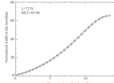
Figure 5. Element of field line separation in the meridian plane for a dipole magnetic field, normalized to the value at the Earth’s sur-face. The full line shows the values obtained by integrating the first order differential equations, while the crosses are obtained from the analytic expression.
analytic values to within the numerical accuracy of the in-tegration process. For example Fig. 5 compares the field line separation in the magnetic meridian (full line) with that com-puted from Eq. (18) (crosses) for a field line starting at 72◦ at a height of 250 km in the ionosphere and finishing at the equatorial plane. The results agree to better than 1 part in 106 for an integration step length of 1RE.
5.2 Electric field mapping in the Harris model
We have tested the validity of the method of field line map-ping that is described in Sect. 3 by using the Harris model. The coding is in Python with the intention of providing a template for an open source package that will be developed for electric field mapping in more realistic magnetic field ge-ometries (Maus et al., 2005; Tsyganenko, 1987, 1995, 1996). The integration process is the same as described above for a dipole. The results for the field line coordinatesxiand nor-malized separationwi are stored in arrays. If we wish to ter-minate at a particular point we specify a function ofs, the distance along the field line that must be zero at the end point. When this function changes sign we take the coordinates of the last two points as the starting values for a regula falsi (Press et al., 1989) process to find the zero of the function. For example, if we choose to end the trace in the ionosphere at an altitude of 250 km we evaluateh−250 at each point along the path. When it changes sign we enter the regula falsi routine. This interpolates linearly between the last two valuess1ands2ofsto find a new values3that is closer to the root. With a step length ofs3−s2the equations are ad-vanced another step to find a newh. This is repeated until
x(RE)
−10 −8
−6 −4
−2 0
2
y(RE)
−6 −5
−4 −3
−2 −1
0 1
z(
RE
)
−4 −3 −2 −1 0
[image:9.612.326.524.67.259.2]1 2 3 4
Figure 6. Field line trace (blue) and electric field mapping (red) in a Harris model withBeq=3.4×10⁴nT,B0=50.0 nT and plasma sheet thicknessd=1.5RE. The trace starts at 70◦latitude, 03:00 LT (local time), and 250 km altitude. The projections of the mag-netic field line and the electric field vectors on the coordinate planes are also shown. Scale of electric field vector: 1 length unit=35.4 mV m−1.
and converges more slowly than a second order process such as the Newton-Raphson method, it requires much less com-putation. In practice it only requires about five or six steps to achieve an accuracy of one part in 106.
Figure 6 shows the results of such a process. A field line is traced from a point in the Northern Hemisphere ionosphere at altitude 250 km, latitude 70◦ and local time 03h00. The parameters of the model (shown in the caption) are chosen to produce a strong tail field. The trace is terminated at an alti-tude of 250 km in the opposite hemisphere. The model is, of course, symmetric about the equatorial plane. The blue line represents the magnetic field line. The effect of the Harris sheet is obvious, with the field line being swept back tail-wards and strong curvature within the plasma sheet. We also show the projection of the field line on each of the coordi-nate planes. The electric field is represented by the red line segments along the field line projections. Each line segment represents the projection of the electric field vector on the coordinate plane.
Because there is strong dependence of the electric field magnitude on radius the field vectors are barely discernable at larger radii. The diagram is not, however, intended to pro-vide a quantitative picture of the electric field mapping but to give a feel for the geometry. A better idea of the variation of
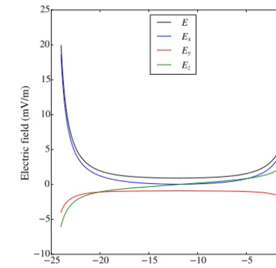
Ealong the field line is given in Figs. 7 and 8. Figure 7 shows magnitude of the electric field and of its three components as
−25 −20 −15 −10 −5 0
Distance along field line (RE) −10
−5 0 5 10 15 20 25
Electric field (mV/m)
E Ex
Ey
Ez
Figure 7. Electric field normalized to the value at the starting point, for the field line traced and electric field mapped in Fig. 6.
a function of s, the distance measured along the field line (negative when in the opposite direction toB). Thex andy components ofEare symmetric about the equator whileEz is antisymmetric. There is strong variation of the magnitude ofE, which varies from 35.4 mV m−1 in the ionosphere to about 0.5 mV m−1near the equator. A better idea of howE
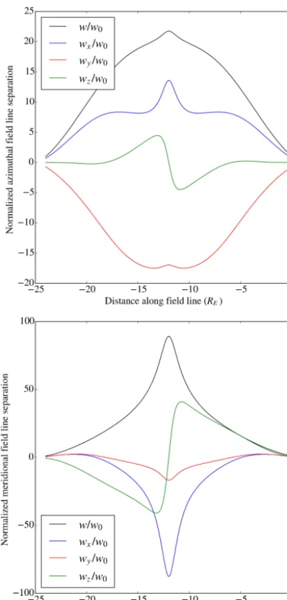
varies near the equator can be obtained by examining Fig. 8. The normalized width vector is in the same direction asE
and its magnitude is proportional to the reciprocal ofE. It is not the intention of this paper to provide the results of a large number of computations in a model that is only in-tended to be illustrative. The purpose is to validate the tech-nique of computation in a relatively simple model. We de-scribe below the various checks that we have made on the accuracy of the integration technique.
5.3 Computational checks of mapping in the Harris model
We have already described how, in a dipole model, we can use the integration technique and compare the results with the explicit formulae presented in the first part of the paper. The agreement is, in all cases, very good. With integration steps of 1.5 to 2.0REagreement between the computed val-ues of positionxiand field line separationwi/w0is typically about 1 part in 106for a dipole model. Larger steps than this increase the truncation error and reduce the accuracy. The step length is best chosen by the user to suit the numerical accuracy of the computer and the requirements of the prob-lem.
[image:9.612.50.287.70.291.2]Figure 8. Element of field line separation in the electric field direc-tion, for the field line traced in Fig. 6.
maintained. As a check against this, at each step, we calcu-late the scalar product of the unit vectors parallel towandB. If its magnitude exceeds a predetermined value an exception is raised and the user can set a better step length. Ultimately, in production versions of the program for realistic models it will be necessary to use a more sophisticated adaptive step integration technique. For the present the simpler technique suffices.
Another check that will be particularly useful in more elaborate models is to take two initial values ofw,w1and
w2, in different directions perpendicular toB. These can both be integrated simultaneously along the field line. Then the cross-section of the flux tube defined by these is w1×w2.
The magnetic flux is constant along the flux tube and we can check this by evaluatingB·w1×w2at each step. In an inte-gration in the Harris model constancy can be maintained to about 1 part in 106with appropriate step length. The compu-tational overhead of integrating three additional equations is too large for this to be useful in routine calculations, but it is very useful in checking the correctness of the coding for the magnetic field model.
6 Discussion and conclusions
In this paper we have introduced a new method of mapping electric fields along geomagnetic field lines. A set of three differential equations for the components of the normalized separation of two field lines has been obtained. These can be integrated simultaneously with the equations that trace the field line. Since the magnetic field lines are equipotentials, this allows the calculation of a component of the electric field as a function of distance measured along the field line. Two values of the normalized separation are required to give two field line components resulting in a total of nine first order differential equations that must be simultaneously integrated. The computational effort in integrating the set of nine equations is the same as that for tracing three field lines. The accuracy of the process is better, however, since finding the electric field by finding the difference between the end posi-tions of the two field lines requires taking small differences of large quantities. Such numerical differentiation is notori-ously inaccurate.
The viability of the method has been carefully tested. The analytic expressions for a number of relevant properties of a magnetic dipole field, while easily derived, are not read-ily available in the literature. We have provided a derivation of these for convenient reference and compared the results calculated from them with those obtained by the integration method. We have also tested the method in a qualitatively more realistic model of the night side magnetosphere. All the tests show that the method is accurate and suitable for mapping in more realistic models. In the accompanying pa-per (Walker, 2016) the process is applied to the International Geomagnetic Reference Field.
Acknowledgements. This work was supported by the South African
National Research Foundation under grant 93068 (SANAE HF Radar), and by the University of KwaZulu-Natal through a research incentive grant.
References
Baker, J. B. H., Greenwald, R. A., Ruohoniemi, J. M., Forster, M., Paschmann, G., Donovan, E. F., Tsyganenko, N. A., Quinn, J. M., and Balogh, A.: Conjugate comparison of Super Dual Au-roral Radar Network and Cluster electron drift instrument mea-surements of E×B plasma drift, J. Geophys. Res., 109, A01209, doi:10.1029/2003JA009912, 2004.
Greenwald, R. A., Baker, K. B., Dudeney, J. R., Pinnock, M., Jones, T. B., Thomas, E. C., Villain, J.-P., Cerisier, J.-C., Senior, C., Hanuise, C., Hunsucker, R. D., Sofko, G., Koehler, J., Nielsen, E., Pellinen, R., Walker, A. D. M., Sato, N., and Yamagishi, H.: DARN/SuperDARN: A global view of high latitude convection, Space Sci. Rev., 71, 761–796, 1995
Harris, E. G.: On a plasma sheath separating regions of oppositely directed magnetic field, Nuovo Cimento, 23, 115–121, 1962. Lyons, L. R. and Williams, D. J.: Quantitative Aspects of
Magneto-spheric Physics, D. Reidel Publishing Company, Dordrecht, Hol-land, 231 pp., 1984.
Maus, S., Macmillan, S., Chernova, T., Choi, S., Dater, D., Golovkov, V., Lesur, V., Lowes, F., Luhr, H., Mai, W., McLean, S., Olsen, N., Rother, M., Sabaka, T., Thomson, A., and Zvereva, T.: The 10th-Generation International Geomagnetic Reference Field, Geophys. J. Int., 161, 561–565, 2005.
Mozer, F. S.: Electric field mapping from the ionosphere to the equatorial plane, Planet. Space Sci., 18, 259–263, 1970.
Press, W. H., Flannery, B. P., Teukolsky, S. A., and Vetterling, W. T.: Numerical Recipes, (FORTRAN version or Pascal version or C version), Cambridge University Press, Cambridge, 818 pp., 1989.
Tsyganenko, N. A.: Global quantitative models of the geomagnetic field in the cislunar magnetosphere for different disturbance lev-els, Planet. Space Sci., 35, 1347–1358, 1987.
Tsyganenko, N. A.: Modeling the Earth’s magnetospheric magnetic field confined within a realistic magnetopause, J. Geophys. Res., 100, 5599–5612, 1995.
Tsyganenko, N. A.: Effects of the solar wind conditions on the global magnetospheric configuration as deduced from data-based field models, European Space Agency Publication ESA SP-389, p. 181, 1996.
Walker, A. D. M.: Magnetohydrodynamic Waves in Geospace: The theory of ULF waves and their interaction with energetic parti-cles in the solar-terrestrial environment, IOP Press, Bristol, UK, 549 pp., 2005.