A new method for solving the MHD equations in the magnetosheath

Ann. Geophys., 31, 419–437, 2013 www.ann-geophys.net/31/419/2013/ doi:10.5194/angeo-31-419-2013

© Author(s) 2013. CC Attribution 3.0 License.

EGU Journal Logos (RGB)

Advances in

Geosciences

Open Access

Natural Hazards

and Earth System

Sciences

Open Access

Annales

Geophysicae

Open Access

Nonlinear Processes

in Geophysics

Open Access

Atmospheric

Chemistry

and Physics

Open Access

Atmospheric

Chemistry

and Physics

Open Access

Discussions

Atmospheric

Measurement

Techniques

Open Access

Atmospheric

Measurement

Techniques

Open Access

Discussions

Biogeosciences

Open Access Open Access

Biogeosciences

Discussions

Climate

of the Past

Open Access Open Access

Climate

of the Past

Discussions

Earth System

Dynamics

Open Access Open Access

Earth System

Dynamics

Discussions

Geoscientific

Instrumentation

Methods and

Data Systems

Open Access

_{Geoscientific}

Instrumentation

Methods and

Data Systems

Open Access

Discussions

Geoscientific

Model Development

Open Access Open Access

Geoscientific

Model Development

Discussions

Hydrology and

Earth System

Sciences

Open Access

Hydrology and

Earth System

Sciences

Open Access

Discussions

Ocean Science

Open Access Open Access

Ocean Science

Solid Earth

Open Access Open Access

Solid Earth

Discussions

The Cryosphere

Open Access Open Access

The Cryosphere

Natural Hazards

and Earth System

Sciences

Open Access

Discussions

A new method for solving the MHD equations in the magnetosheath

C. Nabert1, K.-H. Glassmeier1,2, and F. Plaschke3

1_{Institut f¨ur Geophysik und extraterrestrische Physik, Technische Universit¨at Braunschweig, Germany} 2_{Max Planck Institute for Solar System Research, Katlenburg-Lindau, Germany}

3_{Institute of Geophysics and Planetary Physics, University of California, Los Angeles, CA, USA}

Correspondence to: C. Nabert ([email protected])

Received: 29 November 2012 – Revised: 13 February 2013 – Accepted: 13 February 2013 – Published: 5 March 2013

Abstract. We present a new analytical method to derive

steady-state magnetohydrodynamic (MHD) solutions of the magnetosheath in different levels of approximation. With this method, we calculate the magnetosheath’s density, ve-locity, and magnetic field distribution as well as its geome-try. Thereby, the solution depends on the geomagnetic dipole moment and solar wind conditions only. To simplify the rep-resentation, we restrict our model to northward IMF with the solar wind flow along the stagnation streamline. The sheath’s geometry, with its boundaries, bow shock and magnetopause, is determined self-consistently. Our model is stationary and time relaxation has not to be considered as in global MHD simulations. Our method uses series expansion to transfer the MHD equations into a new set of ordinary differential equations. The number of equations is related to the level of approximation considered including different physical pro-cesses. These equations can be solved numerically; however, an analytical approach for the lowest-order approximation is also presented. This yields explicit expressions, not only for the flow and field variations but also for the magnetosheath thickness, depending on the solar wind parameters. Results are compared to THEMIS data and offer a detailed expla-nation of, e.g., the pile-up process and the corresponding plasma depletion layer, the bow shock and magnetopause ge-ometry, the magnetosheath thickness, and the flow decelera-tion.

Keywords. Magnetospheric physics (Magnetopause, cusp,

and boundary layers; Magnetosheath) – Space plasma physics (Kinetic and MHD theory)

1 Introduction

The magnetosheath is the flow region of the solar wind around the Earth. Its characteristics, for example its thick-ness or magnetic field distribution, depend on the solar wind conditions. In regions without reconnection, the earthward boundary of the flow region, the magnetopause, is defined as a boundary with vanishing normal flow velocity. It is char-acterized as a small region where a transition from magne-tosheath plasma density and temperature to magnetospheric conditions occurs. Very often the magnetopause is identified by an abrupt change in the magnetic field, which is related to a region with spatially confined electric current. Chapman and Ferraro (1930) were the first to speculate about the ex-istence of such a magnetopause current layer. Without a so-lar wind magnetic field, all current is located at the magne-topause, corresponding to a field-free magnetosheath with a jump of the magnetic field at the magnetopause. Therefore, the flow within the magnetosheath can be treated in terms of hydrodynamics (e.g., Spreiter et al., 1966).

A sharp current layer, however, does not always exist at the magnetopause as demonstrated in Fig. 1, showing obser-vations made on-board the THEMIS-C spacecraft. The five spacecraft of the THEMIS mission were launched in 2007 (Angelopoulos, 2008) and provide a wealth of plasma and magnetic field observations suitable for magnetosheath and magnetopause studies (e.g., Glassmeier et al., 2008; Plaschke et al., 2009; Zhang et al., 2009). On 29 October 2009 the THEMIS-C spacecraft traversed the magnetosheath al-most along the stagnation streamline. Measurements by the ESA plasma instrument (McFadden et al., 2008) allow for a clear identification of the magnetopause crossing at 08:25 UT based on abrupt changes of the plasma density and temperature to magnetospheric conditions. Magnetic field

Time [h]

u

(Ion)

x

B

z

Bow Shock Magnetopause

N (Ion)

29.10.2009 THEMIS C

[nT]

0 80 60 40 20

107

106

105

104

[1/cm ]

3

0 40 30 20 10

[km/s]

100 0 -100 -200 -300

0700

0600 0800

Continuous

Sharp Jumps Smooth Increase

Fig. 1. A low-shear magnetopause transition on 29 October 2009.

The upper panel showsBz(GSM) magnetic field observations. The

second panel displays the (ion) velocity in x-direction (GSM), and the third one shows the density of the plasma ions. The last panel depicts the logarithmic ion temperature.

observations by the FGM (Auster et al., 2008), however, re-veal a magnetic pile-up throughout the entire magnetosheath; i.e., the field slowly increases. At the magnetopause, the magnetosheath field smoothly adapts to the magnetospheric field. Thus, there is no confined magnetopause current but currents distributed over the entire magnetosheath. Simi-lar pile-up observations under low-shear conditions were reported by, e.g., Crooker et al. (1979), Paschmann et al. (1993), Phan et al. (1994), or Farrugia et al. (1997). In these earlier reported cases, however, the magnetic pile-up region is usually less extended than in the present case.

A first model to calculate the magnetic pile-up in the mag-netosheath was presented by Lees (1964). In this model, the magnetohydrodynamic (MHD) equations are restricted to ax-isymmetric flows, and the velocity tangential to the stagna-tion streamline is assumed to be a known funcstagna-tion. Although these restrictions strongly limit the scope of the theory, basic aspects of the magnetic pile-up could be investigated. A more detailed theory was developed by Zwan and Wolf (1976), the so-called depletion layer model. They considered a flux tube moving through the magnetosheath in the MHD approach. Zwan and Wolf (1976) concluded that the plasma in the flux tube is squeezed out near the magnetopause, leading to a lowered density and an enhanced magnetic field strength. Note that this consideration leads to a somewhat different density behavior compared to Lees (1964). Another theoret-ical approach is the magnetic string model by Erkaev et al. (1988). In this model, the MHD equations are solved in a new coordinate system, specially designed to take advantage of the frozen-in magnetic field. However, both latter mod-els also rely on additional assumptions (e.g., the pressure

distribution in the magnetosheath) and/or require solutions of more complicated partial differential equations. All these models solve differential equations derived from the MHD equations. Global MHD simulations are another investiga-tion method which solves the complete set of MHD equa-tions directly to obtain a magnetosheath solution as shown by Wu (1984), Wu (1992), Ogino et al. (1992), Siscoe et al. (2002) and Wang et al. (2004), among others.

Simple and very reduced models can provide insight into the basic physical processes underlying a phenomenon. However, more complex models include more processes and can show how the phenomenon is embedded into a com-plex physical environment. One should be aware, however, that numerical effects can strongly influence any result when solving more complex differential equations. Numerical dif-fusion near the bow shock or magnetopause is large in global MHD simulations, as noted by Wu et al. (1981). Subsequent developments on the numerical schemes try to reduce the in-fluence of diffusion; however, it is still a difficult task (Toth, 2000). Only a detailed comparison of simple and complex approaches provides a complete understanding of the phe-nomenon considered.

Here, we present a new analytical method to solve the MHD equations in different orders of approximation, from a lowest-order approach to the complex, full MHD solution. Our approach is able to classify the MHD models introduced above with respect to different levels of approximation. We show that the different results in the density distribution of Lees (1964) and Zwan and Wolf (1976) can be referred back to different levels of approximation used. The method is able to calculate the fluid properties, such as density, pressure, velocity, and magnetic field, as well as the magnetosheath’s geometry bounded by the bow shock and magnetopause. In the lowest-order approach, analytical solutions are obtained, yielding explicit expressions for the density and field distri-bution, as well as for the magnetosheath thickness and its dependence on the solar wind magnetization.

The magnetosheath thickness and the related bow shock distance have been a major topic of investigation for decades, as reviewed by Petrinec (2002). However, only empirical re-lations have been derived (Spreiter et al., 1966) and modified by Farris and Russell (1994) to take the solar wind magnetic field into account. We will compare our analytically derived expression with the empirical relations.

MHD Equations _ParametersSolar Wind

Earth‘s Dipole Description

ODEs Ansatz

Boundary Conditions at

Bow Shock

Rankine-Hugoniot Relations

Additional Conditions Magnetopause

Steady-State MHD Solution

Outflow Conditions

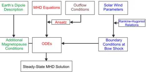
Fig. 2. Overview of the interplay between different aspects of our

model. Each color represents a part discussed in a separate section in this chapter. The top row displays the input for our method.

2 Theory

Physical quantities in the steady-state magnetosheath, such as density, pressure, velocity, or magnetic field, can be de-termined by the stationary MHD equations. They depend on three spatial coordinates (x, y, z). We choose the x-axis to be along the stagnation streamline and the y- and z-axis to be perpendicular to it. The quantities are expanded into power series with respect toy andzaround the stagnation stream-line:f (x, y, z)=f0(x)+f1(x) y+f2(x) z+f3(x) y z+. . ..

Substituting such an ansatz for each quantity in the MHD equations and equating coefficients of the tangential orders (1, y, z, y z, . . . ), a system of ordinary differential equa-tions (ODEs) depending only on the normal directionx is obtained. It is suitable to modify our ansatz with respect to the magnetosheath geometry. Consequently, our system of ODEs and the corresponding solutions depend on bow shock and magnetopause geometry parameters. These parameters are calculated by taking the geomagnetic field into account. Boundary conditions (inflow conditions) for our system of ODEs are determined at the bow shock. The shocked values are referred back analytically to the solar wind conditions using the Rankine–Hugoniot relations. Note that the MHD equations require further boundary conditions (in global MHD simulations called outflow conditions) far away along the y- and z-direction. The complete set of ODEs using the series expansion ansatz to infinite order is not easy to handle. A finite expansion order leads to a finite system of ODEs, which remains underdetermined. But we can use the outflow conditions to close the system. Finally, a solution of the mag-netosheath flow and field quantities as well as the bow shock and magnetopause geometry can be calculated depending on solar wind conditions only. The interplay of the different parts of the model are displayed in Fig. 2.

2.1 Deriving ODEs from MHD

Plenty of phenomena of the plasma flow in the magne-tosheath are described by the ideal MHD theory (e.g., Siscoe et al., 2002). The time-independent (stationary) MHD

equa-x

z

MP

x

BS

MS

Solar

Wind

Solar

Wind

x

Geomagnetic

Dipole

Fig. 3. The incident solar wind in x-direction with its field along the

z-direction on the left side and the Earth with its dipole field on the

right side. The origin of the Cartesian coordinate system (x, y, z)

shall be at the nose of the bow shock (BS).

tions read

∇ ·(ρu)=0, (1)

ρ (u· ∇)u+ ∇p− 1

µ0

(∇ ×B)×B=0, (2)

∇ ×(u×B)=0, (3)

∇ ·B=0, (4)

p=k ργ. (5)

Hereρ denotes mass density,uthe fluid’s bulk velocity,p

the thermal gas pressure (assumed to be isotropic), B the magnetic field,µ0=4π×10−7N/A2the vacuum

permeabil-ity, andγ the ratio of specific heats. Note that instead of the full energy conservation law, an adiabatic law (Eq. 5) is used with the proportionality constantk. The adiabatic law is valid within the magnetosheath, but not through the bow shock due to entropy changes.

The super-magnetosonic solar wind flow causes a bow shock in front of the Earth. A Cartesian coordinate system is used with origin at the bow shock’s nose (subsolar point). The x-axis points towards the Earth, which is located atxE

(see Fig. 3). The bow shock distance to the Earth, that is,xE,

solar wind magnetic field to be parallel (northward or posi-tive) along the z-axis. Furthermore, the Earth’s magnetic field is represented by a dipole, its moment being anti-parallel to the z-axis with magnitudeM=8×1015Tm3. The compo-nents of the geomagnetic fieldBEare given by (e.g., Ogino,

1993)

BE,x=

−3z 1x

r5 M, (6)

BE,y=

−3y z

r5 M, (7)

BE,z=

−2z2+1x2+y2

r5 M, (8)

with the radial distance r=p1x2_+y2_+z2_{, and 1x=}

xE−xdefining the distance from the Earth’s center (Fig. 3).

Note that the solar wind magnetic field and the dipole field are parallel close to the dayside stagnation streamline, which excludes reconnection.

The situation introduced above is highly symmetric. The dipole field has a rotational symmetry with respect to the dipole moment axis, and the solar wind flow is perpendicular to this symmetry axis, leading to symmetric properties in the MHD flow around the dipole field. A detailed discussion of the symmetry relations is presented in Appendix A.

We approximate the bow shock as well as the magne-topause shapes by elliptic paraboloids (functional relation

x=x0+a y2+b z2 with constantsx0,a, andb). This

cor-responds to a second-order series expansion in accordance with the symmetry considerations. The bow shock and mag-netopause parametrization are

x= X

t=y,z

cBS,tt2, (9)

x=xMS+ X

t=y,z

cMP,tt2, (10)

respectively, wherexMS denotes the magnetopause distance

from the bow shock’s nose (which is the magnetosheath thickness along the stagnation streamline, x-axis). The con-stant parameterscBS,t for the bow shock andcMP,t for the magnetopause represent curvatures in the respective tangen-tial directiont=yort=z. These geometric parameters are determined by the interaction of the magnetosheath plasma with the dipole field as we will show later.

The flow and field variables in the magnetosheath are expanded into Taylor series with respect to the y- and z-direction around the stagnation streamline (y=z=0). Due to the symmetry relations summarized in Table A1 (Ap-pendix A), several expansion terms vanish. This leads to the following ansatz expanded to the third order:

ρ=ρ0+ρ20y2+ρ02z2, (11)

p=p0+p20y2+p02z2, (12)

Bx=Bx01z+Bx21y2z+Bx03z3, (13)

By=By11y z, (14)

Bz=Bz0+Bz20y2+Bz02z2, (15)

ux=ux0+ux20y2+ux02z2, (16)

uy=uy10y+uy12y z2+uy30y3, (17)

uz=uz01z+uz21y2z+uz03z3. (18)

Note that the expansion only holds for the tangential direc-tions. Thus, the coefficients are arbitrary functions ofx. Their indices indicate the order inyandz; e.g., “20” means second order inyand zeroth order inzand “0” means zeroth order inyandz.

Due to the curved shape of the bow shock and magne-topause, coefficient functions are more conveniently depend-ing onx˜ instead ofx (e.g.,ρ0(x)→ρ0(x)˜ ), withx˜ defined

by the following relation:

x= ˜x+ X

t=y,z

cBS,t+1ct ˜

x xMS

t2, (19)

where 1ct =cMP,t−cBS,t denotes the difference between the magnetopause curvature and the bow shock curvature. Each value forx˜ corresponds to an elliptic paraboloid de-fined by Eq. (19). In particular, x˜=0 corresponds to the bow shock parametrization (Eq. 9) andx˜=xMSto the

mag-netopause parametrization (Eq. 10). Therefore, the mod-ified ansatz describes the physical quantities on elliptic paraboloids parametrized by x˜, starting at the bow shock forx˜=0 and finishing at the magnetopause atx˜=xMS(see

Fig. 4). Note that the modification of the ansatz does not af-fect its symmetry becausex˜depends ony2andz2only and, thus,x(y, z)˜ is independent of the sign ofy andz. This can be seen solving Eq. (19) with respect tox˜. Thus, the ansatz still satisfies the symmetry relations given in Table A1.

Substituting our ansatz into the MHD system (1)–(5) yields a set of ordinary differential equations (ODEs) by equating the coefficients of zeroth order,

(ρ0ux0)0+ρ0 uy10+uz01

x

z

Magnetopause x=xMS

Bow Shock x=0

~ 0<x<x~ MS ~

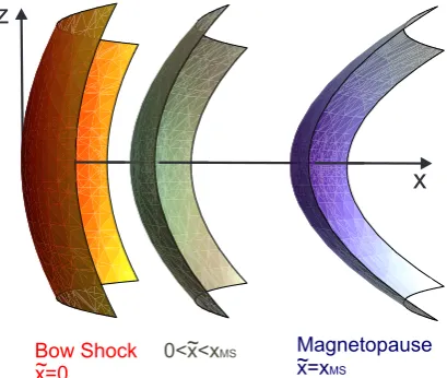
Fig. 4. Three-dimensional sketch of the elliptic paraboloids

de-scribed by Eq. (19) for differentx˜. The bow shock on the left side

forx˜=0 and the magnetopause on the right side forx˜=xMS.

(Bz0ux0)0+Bz0uy10=0, (21)

ρ0ux0u0x0+p 0

0+Bz0Bz00 −Bx01Bz0=0, (22)

p0=k ρ₀γ, (23)

and first order,

B_x010 +2Bz02+By11−2c˜zBz00 =0, (24)

ρ0ux0u0y10+ρ0u2y10+2(p20+Bz0Bz20)−By11Bz0 (25)

−2c˜y p00+Bz0Bz00 ₌

0,

ρ0ux0u0z01+ρ0u2z01+2p02+Bx012 −Bx01Bz00 (26)

−2c˜zp00=0,

p20=k γ ρ20ργ −1

0 , (27)

p02=k γ ρ02ργ −1

0 , (28)

By11ux0+2(Bz02ux0+Bz0ux02) (29)

−Bx01 uy10+2uz01+2c˜zBz0uy10=0,

withc˜t=cBS,t+1ct_xx˜

MS. Derivatives with respect tox˜ are marked with a prime. To simplify the reading of the equa-tions, we setµ0=1. Equations obtained from equating

co-efficients of the second order can be found in Appendix B. We expressed the series expansion of the MHD quantities in new coordinatesx, y, z˜ . However, as the MHD equations are explicitly expressed in Cartesian coordinates, the chain rule was applied to compute the derivatives with respect to

˜

x, e.g.,∂xp=p0∂xx˜. The factor∂xx˜can be calculated from

Eq. (19):

∂xx˜=1− X

t=y,z

1ct

xMS

t2+O(t4). (30)

Here t4 denotes any fourth-order product ofy and z. The system of equations presented contains a conservation equa-tion (Eq. 29), which has been satisfied by boundary condi-tions only, as it does not contain any derivatives. We denote Eqs. (20)–(23) as the zeroth-order system, Eqs. (20)–(28) as the first-order system, and Eqs. (20)–(28) and (B1)–(B7) as the second-order system.

Our ansatz transforms the stationary MHD equations, which are partial differential equations (PDEs), into a set of ordinary differential equations: (20)–(28) and (B1)–(B7). Al-though the number of equations increases, the numerical ef-fort to solve ordinary differential equations (ODEs) is sig-nificantly lower. Hence, for a sufficient order the solution might be obtained with less effort. The second-order system presented here contains 16 ODEs, depending on 22 coeffi-cient functions and 5 geometric parameters. Thus, 6 addi-tional equations are required to calculate all coefficient func-tions, and 5 additional conditions are needed to determine the geometric parameters.

2.2 Solar wind at the bow shock boundary

First-order derivatives of the coefficient functions with re-spect tox˜ in the above ODEs require knowledge of corre-sponding boundary values at one pointx˜0=0, i.e.,ρ0(x˜0),

ρ20(x˜0),ρ02(x˜0),. . . . We choose to set these values atx˜0=0

(bow shock) using shocked solar wind parameters. These are related to the solar wind via Rankine–Hugoniot relations (e.g., Petrinec and Russell, 1997):

ρ uξ

=0, (31)

Bξ=0, (32)

"

ρ u2_ξ+p+ B

2 τ 2µ0

#

=0, (33)

ρ uξuτ−

Bξ

µ0

Bτ

uξBτ−uτBξ=0, (35)

"

ρ

2u

2₊

_γ

γ−1

p+B

2 τ

µ0 !

uξ−

Bξ

µ0

Bτuτ

#

=0. (36)

The squared brackets[. . .]indicate that the quantity therein is conserved across the shock. The subscriptξ denotes the normal component andτtangential components with respect to the bow shock. Solving the Rankine–Hugoniot relations with respect to the bow shock geometry (Eq. 9) and the cho-sen solar wind conditions, the shocked values are obtained. Power series expansion in y- and z-direction of this solution and equating coefficients with our ansatz determine the coef-ficient functions of the ansatz atx˜=0. Analytical solutions for the zeroth-order coefficients can be found in, e.g., Siscoe (1983). A brief summary of his work and a detailed analyti-cal approach for the the higher-order coefficient values up to the second order are given in Appendix C.

As a result, the velocity coefficients are given by

ul i j(x˜=0)=fu(i, j )2i+jci_BS,ycj_BS,z1u, (37) where1u=uSW−ux0(x˜=0),l∈ {x, y, z},i andj are

la-beled as in Eqs. (16)–(18), andfu(i, j )is defined by (sign-function)

fu(i, j )=

+1, i+j ∈ {1}

−1, i+j ∈ {2,3}. (38) The magnetic field coefficients are given by:

Bl i j(x˜=0)=fB(i, j )2i+jciBS,yc j

BS,z1B, (39)

in which

fB(i, j )=

+1, i+j∈ {1,2}

−1, i+j∈ {3} , (40) where1B=BSW−Bz0(x˜=0),l∈ {x, y, z}, andiandjare

as in Eqs. (13)–(15). The boundary values for the density and pressure coefficientsρ20,ρ02,p20, andp02are

approxi-mately zero.

2.3 Outflow boundary conditions

Since the MHD system (1)–(5) contains partial derivatives with respect to all three space dimensions, boundary condi-tions are needed for three linearly independent planes. In the previous section, boundary conditions were defined for the bow shock plane; these are commonly called inflow condi-tions in global MHD simulacondi-tions. Here the remaining set of outflow boundary conditions are defined, used to close the system of ODEs.

The higher-order coefficient functions in the series expan-sion dominate far away from the stagnation streamline (e.g.,

ρ(x, y˜ → ∞, z→ ∞)≈ρ20(x) y˜ 2+ρ02(x) z˜ 2). We suggest

setting the highest-order coefficients to their bow shock boundary values. This condition is similar to common out-flow boundary condition in simulations (e.g., Ogino, 1993). Different, specific choices of explicit functional relations to close the system of ODEs lead basically to the models by Lees (1964) and Zwan and Wolf (1976), as discussed below.

2.4 Conditions from the geomagnetic field as an obstacle

Despite the boundary conditions introduced above, the sys-tem of ODEs still contains five undetermined geometric pa-rameters: the bow shock curvaturescBS,yandcBS,z, the

mag-netopause curvaturescMP,yandcMP,z, and the magnetosheath

thickness xMS. To determine these, inner boundary

condi-tions are necessary.

First, the flow should be tangential with respect to the magnetopause, not allowing flow to penetrate into the mag-netosphere (e.g., Biernat et al., 1999). This stems from the definition of the magnetopause as earthward flow bound-ary. The flow direction at the magnetopause can be cal-culated using magnetopause surface coordinates. The nor-mal magnetopause vector is derived from the magnetopause parametrization (10):

ξMP=

1

nMP

1,−2cMP,yy,−2cMP,zzT, (41)

wherenMP= q

1+P

t=y,z4c2MP,tt2normalizes the vector. A vanishing normal flow velocity through the magnetopause yieldsξMP·u(x˜=xMS, y, z)=0. This expression holds for

the y- and z-direction, so using the velocity ansatz (16)–(18) yields

ux0(x˜=xMS)=0, (42)

cMP,y=

ux20(x˜=xMS)

2uy10(x˜=xMS)

, (43)

cMP,z=

ux02(x˜=xMS)

2uz01(x˜=xMS)

. (44)

However, at the magnetopause surface the flow velocity van-ishes along the magnetic field direction (→uz01(x˜=xMS)=

et al., 1999). This requires

cMP,z=

Bx01(x˜=xMS)

2Bz0(x˜=xMS)

. (45)

Secondly, a restricting condition arises from the Earth’s dipole field itself. The total magnetic field of our MHD so-lution (B) should by a superposition of the magnetic fields generated by magnetosheath currents (Bj) and the Earth’s magnetic field (BE). Since the Earth’s dipole field is

curl-free (see Eqs. 6–8), the curl of the total field yields the current distribution in the magnetosheathjMSonly:

∇ ×B= ∇ ×Bj=µ0jMS. (46)

The magnetic field generated by these currents can be cal-culated with Biot-Savart’s law. The superposition of this magnetosheath-current-field and the Earth’s magnetic field necessarily has to match the total field from our MHD so-lution. If this is not satisfied, geometric parameters and the magnetopause distance to the Earth’s center have to be mod-ified accordingly.

A more simple approach to take the geomagnetic field into account uses a pressure condition at the magnetopause which is valid in the hydrodynamic limit. Mead and Beard (1964) pointed out that the tangential components of the total mag-netic field determine the (calculated) total pressure behind the magnetopauseptot,MP:

ptot,MP=

ξMP× BE+Bj2

2µ0

. (47)

With respect to Mead and Beard (1964), a good first approx-imation for the right-hand side yields:

ptot,MP=

(fBE×ξMP)2

2µ0

, (48)

with f =2.44. This expression is valid near the stagna-tion point and determines the magnetopause distance to the Earth’s center. Variations in y- and z-direction give additional conditions for determination of two curvature parameters.

Hence, the conditions of vanishing normal flow and field component and the condition for the Earth’s magnetic field determine the geometric parametersxMS,cMP,y,cMP,z,cBS,y

andcBS,z. The differential equations together with the closure

conditions for the highest-order coefficients and the inner boundary conditions determine a unique solution for given solar wind parameters.

2.5 Application of the method

To calculate magnetosheath solutions with our method, first an appropriate order of approximation has to be chosen. For example, the second-order model gives a good approxima-tion of the dayside magnetosheath up to severalRE beside

the stagnation streamline. If the solar wind is along the stag-nation streamline (i.e., the x-direction) with a perpendicular, northward IMF, we can directly apply the ODEs presented here. The system of ODEs related to the zeroth order is given by Eqs. (20)–(23). The second-order approach is given by Eqs. (20)–(28) and (B1)–(B7) as presented in Sect. 2.1 and Appendix B. For solar wind conditions violating the required symmetry conditions, ansatz (11)–(18) has to be replaced by an arbitrary series expansion. However, the derivation of the corresponding ODEs is analogous. Further, higher-order ap-proximations require higher-order series expansions. We set the coefficient functions of the highest-order constant at their postshock values to close the system of equations (i.e., for the second-order approach presented,uy30,uy12,uz03,uz21,

Bx30, andBx21are constant). The boundary conditions for the

ODEs (ρ(x˜=0), p(x˜=0),u(x˜=0), andB(x˜=0)) are de-termined at the bow shock by solving the Rankine–Hugoniot relations for the solar wind conditions (ρSW, pSW,uSW, and BSW) with respect to the shock geometry. However, we can

also use the analytical approach presented in Appendix C yielding equations for zeroth-order coefficients (Eqs. C1– C4) and for the higher-order coefficients (Eqs. C19 and C27). The second-order terms of density and pressure vanish in this approach.

The Rankine–Hugoniot relations as well as the ODEs re-quire knowledge of the geometric parameters xMS, cMP,y,

cMP,z,cBS,y, andcBS,z. As an initial choice, we can use the

an-alytical expressions (D13), (D24), (D28), (D25), and (D29) with the magnetopause distance (Eq. D23). They are related to solar wind conditions via Eqs. (C1)–(C4). The solution of our system has to satisfy the inner boundary conditions given by Eqs. (42), (43), (45), and (48). The latter condi-tion holds for the y- and z-direccondi-tion. The geometric param-eters need to be determined self-consistently; i.e., the initial choice has to be modified until the conditions are satisfied. Note that higher-order expansions of the bow shock and mag-netopause curvatures contain more parameters and lead to more inner boundary conditions. The zeroth- and first-order systems are not able to determine the geometric parameters self-consistently.

Each system of equations together with the boundary and closure conditions represents a distinct approach to obtain a magnetosheath solution, characterized by the order of the system and corresponding level of approximation.

3 Relations to other models

complete derivation is presented in Appendix D. In the fol-lowing section, we focus on an important result of this calcu-lation: the analytical expression for the magnetosheath thick-ness. Furthermore, we show that the models by Lees (1964), Zwan and Wolf (1976), and Erkaev et al. (1996) are included in our new method for different orders of approximation.

3.1 Analytical expression for the magnetosheath thickness

As presented in Appendix D, an analytical expression of the magnetosheath thickness can be found in the zeroth-order approximation that is solely dependent on solar wind con-ditions. This expression is given by

xMS=

1xMP

4

5+mBS

(gu−1)−1

, (49)

wheregu=uSW/ux0(0), the subsolar velocity jump at the

bow shock, which is introduced in Appendix C (Eq. C3) as a function of solar wind conditions. Furthermore, the mag-netopause distance to the Earth’s center1xMP is given as a

function of solar wind conditions in Eq. (D23), andmBSis a

measure for the solar wind magnetization given by

mBS=1−

1 1+γ

2 p0(0) pmag(0)

. (50)

Herepmag(0)=B_z02(0)/2µ0is the postshock magnetic

pres-sure andγ=5/3 is the ratio of specific heats. The magne-tosheath thickness is proportional to the magnetopause dis-tance to the Earth’s center. A typical value for the mag-netopause distance is about 10RE; therewith, the

magne-tosheath thickness results in 2.3RE in the hydrodynamic

limit (mBS=1) for high Mach numbers (gu=4). The mag-netosheath thickness increases with solar wind magnetic field. It should be noted that the sheath thickness may be-come negative in Eq. (49). This occurs for very low Mach number conditions, for which conditions our approximation is not valid. A very often used empirical relation based on hydrodynamic considerations (Spreiter et al., 1966) is

xMS=1.1

1

gu

1xMP. (51)

This equation offers the same proportionality between mag-netosheath thickness and magnetopause distance. Farris and Russell (1994) modified this relation and obtained

xMS=1.1

(γ−1)M₁2_,SW+2

(γ+1) (M₁2_,SW−1)1xMP, (52)

whereM1,SW is the solar wind magnetosonic Mach number

(see also, Bennett et al., 1997). Figure 5 shows a comparison between this relation and Eq. (49). The upper panel shows the magnetosheath thickness as a function of the unmagnetized

1

2

3

4

5

6

7

8

1

2

3

4

5

0

2

4

6

8

1

2

3

4

D

x

MS

[RE]

r

[ /cm³]

m

B

[nT]

D

x

MS

[RE]

Fig. 5. Magnetosheath thickness of our model by Eq. (49) (blue

curves) in comparison to the model by Farris and Russell (1994) (red curves). The upper plot shows the density dependence of

the sheath thickness foruSW=400 km s−1,TSW=2×105K, and

BSW=0 nT. The lower panel offers the magnetic field

depen-dence foruSW=400 km s−1,TSW=2×105K, andρSW=8.4×

10−21kg m−3=5 m_Pcm−3.

solar wind’s density. The relations are similar; however, an offset of about 20 % is observed. In the lower panel, both re-lations’ dependence on solar wind magnetic field are shown. Eq. (49) yields a steeper increase in the sheath’s thickness. However, for tyical solar wind conditions both relations pro-vide a similar magnetosheath thickness, in accord with ob-servations. Thus, Eq. (49) is a suitable analytical expression for the magnetosheath thickness as a function of solar wind conditions.

3.2 The Lees approach

Lees (1964) presented a first model considering the effects of a solar wind magnetic field on the magnetosheath on the stagnation streamline. Starting from ideal MHD and con-sidering the same solar wind conditions, he derives equa-tions similar to our zeroth-order differential equaequa-tions (20)– (23). Note that these equations do not depend on the bow shock and magnetopause geometry. Neglecting the magnetic shear (→Bx01Bz0=0) and assuming an axisymmetric flow

equations. As noted, a relation to close the system is re-quired. He suggested determining the divergence function

uy10 as part of the solution along the magnetopause away

from the stagnation streamline without going into details. Lees’s model is a zeroth-order approach to the flow problem; we extended his considerations by calculating analytical so-lutions presented in Appendix D. As shown in our approach, higher-order differential equations allow for a self-consistent determination of the divergence functions influencing the so-lution.

3.3 The depletion model

The depletion model by Zwan and Wolf (1976) investi-gates, in more detail, density and magnetic field variations on the stagnation streamline and also in its vicinity. Starting from the time-dependent ideal MHD equations, they derive a system of two-dimensional partial differential equations describing the properties of a magnetic flux tube moving through the magnetosheath. Approximations such as WBK and Taylor expansion restrict the calculations to the vicinity of the stagnation streamline. Although the model by Zwan and Wolf (1976) depends on several limiting assumptions, the picture of the pile-up process was deepened. They con-clude that during northward IMF plasma is squeezed out of flux tubes close to the magnetopause, inducing a density de-crease corresponding to a magnetic field inde-crease in order to maintain pressure balance. The region of density decrease, called the depletion region, is narrower than predicted by Lees’s simple model. In the model of Zwan and Wolf (1976), initial postshock divergence values also need to be deter-mined, similarly to our model. However, they obtain these values from numerical hydrodynamic calculations after Spre-iter et al. (1966). To close their system, the functional relation of the pressure is assumed to match the hydrodynamic simu-lations, too. If we applied the same pressure condition to our model, we would achieve closure of our first-order system (20)–(28). This suggests a correspondence of our first-order system with the model of Zwan and Wolf (1976) despite the approaches in solving the MHD system of equations being rather different (we solve only ODEs). Note that the second-order velocity coefficient functions of our model do not con-tribute to the first-order equations and thus do not need to be determined.

3.4 The magnetic string approach

The magnetic string approach by Erkaev et al. (1988) trans-fers the stationary ideal MHD equations into a different set of partial differential equations (PDEs), using so-called ma-terial coordinates (e.g., Erkaev et al., 2003). These coordi-nates are similar to frozen-in coordicoordi-nates, with directions along the flow velocity, the magnetic field, and the electric field (Pudovkin and Semenov, 1977b). These coordinates are preferably used in ideal MHD due to the frozen-in theorem.

The MHD equations can be simplified assuming the total pressure given in the entire magnetosheath, which leads to a set of two-dimensional PDEs that describes thin magnetic flux tubes. Similar to our method, a parametrized bow shock is used. The bow shock and the magnetopause curvatures are calculated self-consistently using magnetopause bound-ary conditions. These conditions are a vanishing normal ve-locity and magnetic field component, and they assume that the pressure satisfies the Newtonian approximation (Petrinec and Russell, 1997). The magnetic string approach was used to investigate the magnetic barrier region, which is equivalent to the depletion layer region. It was applied to the magne-tosheath region of Earth (Farrugia et al., 1997), Venus (Bier-nat et al., 1999), and Jupiter (Erkaev et al., 1996). Further considerations with respect to anisotropic pressure are pre-sented by Erkaev et al. (2000).

4 Application to THEMIS observations

We apply our method to two different scenarios: The hydro-dynamic magnetosheath transition – i.e., the solar wind mag-netic field is zero – and the magmag-netic pile-up transition as shown in Fig. 1, where the solar wind is significantly magne-tized.

4.1 Hydrodynamic transition

Without a solar wind magnetic field, we expect a field-free magnetosheath and results comparable to the hydrodynamic calculations by, e.g., Spreiter et al. (1966). We choose the solar wind velocity to beuSW=310 km s−1, the solar wind

density ρSW=1.34×10−20kg m−3, the solar wind

mag-netic field BSW=0.02 nT, and the solar wind temperature

TSW=1.75×105K. These conditions agree with actual solar

wind conditions during THEMIS C’s crossing of the mag-netosheath region on 24 August 2008. The probe traversed the magnetosheath about 5.5RE in y-direction and about

2RE in z-direction away from the stagnation streamline

(RE=6371 km). Solar wind measurements were obtained by

THEMIS B, which was closely following THEMIS C. We apply our method to this event using the analytical (zeroth-order) approach presented in Appendix D, the full zeroth-order approach with the equations solved numerically, and the second-order approach. The results of the calcula-tions and the THEMIS C observacalcula-tions on 24 August 2008 are displayed in Fig. 6. The numerical zeroth-order ap-proach yields the smaller magnetosheath thickness. The an-alytical and second-order approach (solutions on the stagna-tion streamline) yield comparable thicknesses. The observed magnetosheath thickness, however, is about 0.4RE larger.

r

0.0 0.5 1.0 1.5 2.0 2.5 3.0 0

10 20 30 40

[m

/cm

]

p

3

0

0 20 40

0 20 40 60 80

u

[km/s]

x0

X [R ]MS E 100

B

[nT]

z0

Fig. 6. Magnetosheath solutions on the stagnation streamline for the

analytical (green), the numerical zeroth order (red), and the second order approach (blue). The second-order solution on the probe’s or-bit (close to but not exactly on the stagnation streamline) is shown in black, the corresponding THEMIS data of 24 August 2008 in grey.

The analytical magnetic field diverges at the magne-topause, due to the linear approximation of the velocity’s x-component. A slight density increase is apparent in all so-lutions but the analytical one. This results from the conver-sion of dynamic pressure, neglected only in the analytical calculations, into gas pressure. However, the measured den-sity increases at a higher rate than that given by the models, which is attributed to a density increase in the solar wind density of about 15 % during the observation time. All cal-culated velocities decrease nearly linearly. On the stagnation streamline the velocity’s x-component vanishes, but close to it a finite value remains, vanishing after the magnetopause. This behavior is in accord with the measured data.

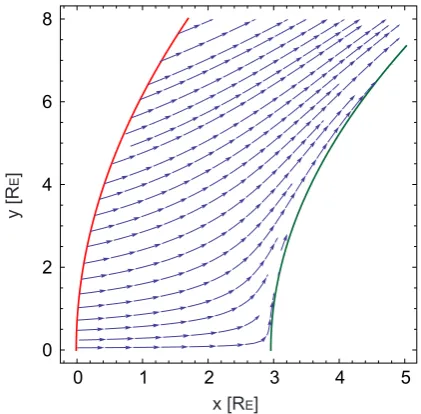
The second-order approach reveals the velocity distribu-tion within the three-dimensional magnetosheath geometry. The corresponding streamlines in the xy-plane are displayed in Fig. 7. The density distribution in the xy-plane is shown in Fig. 8, which shows a decreasing density away from the stagnation streamline. Although these density variations ap-pear to be small, corresponding pressure gradients affect the solution significantly.

The results presented are in agreement with the THEMIS observations as well as numerical calculations by Spre-iter et al. (1966) over a large part of the dayside magne-tosheath. Our three-dimensional solution of the second-order approach with self-consistently computed bow shock and magnetopause geometries yields results that best match the observations of all models considered.

4.2 Northward IMF transition

Without magnetic reconnection, the IMF piles up in the mag-netosheath against the magnetopause. THEMIS C observa-tions on 29 October 2009 (Fig. 1), showing such a pile-up,

0 1 2 3 4 5

0 2 4 6 8

y [R

]

E

x [R ]E

Fig. 7. Magnetosheath streamlines with the velocity obtained by

solving the second-order approach. The parabolic bow shock (red) and the magnetopause (green) are delineated.

0 1 2 3 4 5

0 2 4 6 8

y [R

]

E

x [R ]E

29 33

31

[m

/cm³]

p

Fig. 8. Magnetosheath density distribution obtained by solving the

second-order approach. The parabolic bow shock (red) and the mag-netopause (green) are delineated.

0400 0500 0600 0700 0800 40

30 20 10 0 0 2 4 6

r[m

/cm

]

p

3

r

[m

/cm

]

p

3

SW

UT

Fig. 9. The solar wind density measured by THEMIS B and the

density measured by THEMIS C crossing the bow shock several times. The absolute values of the solar wind density do not fit well. This might be explained by a non-vanishing spacecraft potential; however, the relative variations can be considered. Note that the density jump measured by THEMIS C at about 05:30 UT is related to a mode change of the ESA plasma instrument of the spacecraft (McFadden et al., 2008).

and the satellite’s trajectory is located close to the stagna-tion streamline (distance less than 2RE) as required for our

method in the approximations presented here. However, the solar wind density varied significantly during the observation time, which violates the assumed stationarity of our model with the consequences discussed below. Time-shifted solar wind (ion) density measurements (observed by THEMIS B) and corresponding THEMIS C density measurements, both obtained by the on-board ESA plasma instrument (McFad-den et al., 2008), are shown in Fig. 9. Immediately after the first two bow shock crossings at 04:30 UT and 04:50 UT, the solar wind density increases, causing an inward motion of bow shock and magnetopause. Consequently, the THEMIS C spacecraft reenters the solar wind at about 05:00 UT.

The bow shock distance to the Earth’s center and that of the magnetosheath thickness of the second-order solution are shown in Fig. 10. Both quantities decrease with increasing density. This is also consistent with the results of our an-alytical approach (Eqs. 49 and D23). Additionally, Fig. 10 shows that the effect of the magnetic field variability during the event discussed is negligible when compared to changes in density.

As can be seen in Fig. 9, a solar wind density decrease preceded the bow shock crossing of THEMIS C at 06:05 UT. This causes an outward motion of the bow shock. Therefore, the velocity behind the bow shock shown in Fig. 1 is about 20 km s−1_{lower than expected by the Rankine–Hugoniot}

re-lations (Eqs. 31–36), which are only valid for a stationary situation. Consequently, the bow shock and magnetopause position and the magnetosheath thickness varied during the first part of the observation. For this reason, the length scales of the observations might not be comparable to our calcula-tions. The results of our analytical approach, our zeroth-order as well as our second-order approach are presented in Fig. 11. In all cases, a magnetic pile-up is predicted. As explained by Siscoe et al. (2002), the magnetosheath plasma at the

mag-æ æ æ æ æ æ

4

5

6

7

8

9

14.5

15.0

15.5

16.0

16.5

æ

æ

æ

æ

æ

æ

D

X [R

]

E

r

_{[m /cm ]}

4.5 nT

5.5 nT

BS

æ æ æ æ æ æ

3.4

3.6

3.8

4.0

4.2

4.4

4.6

æ

æ

æ

æ æ

æ

X[

R

]

E

MS

4.5 nT

5.5 nT

Fig. 10. Calculations of the bow shock distance from the Earth’s

center and the magnetopause thickness as a function of the solar wind density, using the second-order approach. Two different solar wind magnetizations, 4.5 nT and 5.5 nT, were considered.

0 1 2 3 4

20 30 40 50

20 10 0

0 20 40 60 80

r[m

/cm

]

p

3

0

u

[km/s]

x0

B

[nT]

z0

X [R ]MS E

Fig. 11. Magnetosheath solutions on the stagnation streamline for

the analytical (green), the numerical zeroth-order (red), and the second-order approach (blue).

Again, the magnetic field of the analytical approach di-verges at the magnetopause due to the linear velocity ap-proximation made. Furthermore, the numerical zeroth-order approach shows the most-extended sheath thickness. This be-havior is associated with a slow density decrease, which con-trasts with the density drop at the magnetopause in the other calculations. The solution of the zeroth-order system is com-parable to that of the Lees (1964) model, which exhibits the same slow density decrease, whereas the second-order solu-tion is similar to the solusolu-tion by Zwan and Wolf (1976). The pressure gradients in the second-order approach enhance the plasma flow away from the stagnation streamline close to the magnetopause. Consequently, the depletion layer thickness, which is given by the density decrease at the magnetopause, differs.

It can be shown that the often-used empirical magne-topause model by Shue et al. (1998) and the bow shock model by Bennett et al. (1997) provide approximately the same curvatures as our theoretical approach. Furthermore, the second-order approach offers a well-known behavior: The divergence of the velocity along the magnetic field drops at the magnetopause. This is related to the fact that the stag-nation point is extended to a line along the magnetic field at the magnetopause as discussed by Pudovkin and Semenov (1977a).

5 Conclusions

A method to calculate the properties of the magnetosheath as part of the solar wind–geomagnetic field interaction by solving the stationary MHD equations for different levels of approximation is presented. The solutions are calculated without considering time relaxation into a stationary state, as required, for instance, by MHD simulations. A power series ansatz is introduced which transfers the stationary MHD equations into a set of ordinary differential equations (ODEs). The number of equations is determined by the order of approximation considered in the ansatz. In the process, for simplicity, we restricted the approach to northward IMF and a solar wind along the stagnation streamline. The postshock values, used as boundary conditions for the ODEs, are re-ferred back to solar wind conditions via Rankine–Hugoniot relations. Furthermore, typical outflow boundary conditions are chosen to determine a unique solution. The Earth’s dipole field yields additional restrictions for the solution determin-ing the magnetosheath’s geometry.

A full analytical solution of our zeroth-order approach is presented, which results in an analytical expression of the magnetosheath thickness (Eq. 49). The models by Lees (1964), Zwan and Wolf (1976), and Erkaev et al. (1988) are classified by different orders of approximation with re-spect to our method, revealing similarities and differences and providing a more detailed insight into magnetosheath phenomena.

Table A1. Symmetries of the situation considered.

Axisymme-try of a quantityf (x, y, z)to the xy-plane means f (x, y,−z)=

f (x, y, z), point symmetry meansf (x, y,−z)= −f (x, y, z), anal-ogous with respect to the xz-plane.

Phys. quantity Symmetry toxy Symmetry toxz

Bx axisym. pointsym.

By pointsym. pointsym.

Bz axisym. axisym.

ux axisym. axisym.

uy pointsym. axisym.

uz axisym. pointsym.

ρ axisym. axisym.

p axisym. axisym.

We apply our method to THEMIS observations. First, a hydrodynamic transition is examined featuring the typical Chapman-Ferraro picture of a jump in the magnetic field at the magnetopause. The second transition investigated shows an extended magnetic pile-up region resulting from a sig-nificantly magnetized solar wind. Model results in terms of streamline distribution, the density contours, the magnetic field behavior, and the magnetosheath geometry validate our approach.

We are currently exploring the possibility to generalize our approach to situations at other planetary bodies such as comets (Glassmeier et al., 2007) or asteroids (Auster et al., 2010).

Appendix A

Symmetry relations

The symmetry relations of the MHD variables with respect to the xy- and xz-coordinate planes are summarized in Ta-ble A1.

In the following, we sketch the derivation of these rela-tions. In Sect. 2.1, we assume the solar wind to flow along the x-axis with its magnetic field along the z-axis and the Earth’s dipole field given by Eqs. (6)–(8). Both the undisturbed solar wind and the dipole field satisfy the symmetry relations. The time evolution of the flow is governed by the time-dependent MHD equations, which read (e.g., Wu, 1992)

˙

ρ+ ∇ ·(ρu)=0, (A1)

ρu˙+ρ (u· ∇)u+ ∇p− 1

µ0

(∇ ×B)×B=0, (A2)

˙

∇ ·B=0, (A4)

˙

+∇ ·

ρu2

2 +

γ γ−1p

!

u− 1

µ0

(u×B)×B !

=0. (A5)

Hereρ denotes mass density,uthe fluid’s bulk velocity,p

the thermal gas pressure assumed to be isotropic,Bthe mag-netic field,µ0=4π×10−7N/A2the vacuum permeability,

and=ρu2/2+B2/(2µ0)+p/(γ−1)the energy density

withγas the ratio of specific heats. Time derivatives are pre-sented in dot notation. The time-dependent MHD equations conserve the symmetry relations in time. For example, ap-plying the relations, the divergence term of the first MHD Eq. (A1) is axisymmetric with respect to the xy-plane as a function ofzand axisymmetric with respect to the xz-plane as a function of y. Thus, Eq. (A1) requires the density to be axisymmetric in time. Because the initial situation (solar wind and Earth’s magnetic field) satisfies the symmetry rela-tions and these relarela-tions are conserved in time, the solution in its final stationary state needs to satisfy the symmetries, too.

Appendix B

Second-order equations

The ansatz (11)–(18) is expanded up to the third order. Sub-stituting this ansatz in the MHD equations, we derived the zeroth- and first-order equations as presented in Sect. 2.1. Analogously, the second-order equations are obtained by equating coefficients of the second order:

(ρ0ux20+ρ20ux0)0+ρ0 3uy30+uz21 (B1)

+ρ20 3uy10+uz01−2c˜y ρ0uy10 0

−1cy

xMS

(ρ0ux0)0=0,

(ρ0ux02+ρ02ux0)0+ρ0 uy12+3uz03 (B2)

+ρ02 uy10+3uz01−2c˜z(ρ0uz01)0

−1cz

xMS

(ρ0ux0)0=0,

Bx01uy10−By11ux0 0

+2 Bz02uy10+Bz0uy12 (B3)

−2By11uz01−2c˜z Bz0uy10 0

=0,

−(Bz0ux20+Bz20ux0)0−3 Bz20uy10+Bz0uy30 (B4)

+2c˜y Bz0uy10 0

+1cy

xMS

(Bz0ux0)0=0,

(Bx01uz01−Bz0ux20−Bz02ux0)0−Bz02uy10 (B5)

−Bz0uy12+By11uz01+

1cz

xMS

(Bz0ux0)0=0,

ρ0(ux0ux20)0+ρ20ux0u0x0+2ρ0ux20uy10+p020 (B6)

+(Bz0Bz20)0−Bx21Bz0−Bx01Bz20

−2c˜yρ0uy10u0x0−

1cy

xMS

Bx01Bz0=0,

ρ0(ux02ux0)0+ρ02ux0ux00 +2ρ0ux02uz01+p020 (B7)

+(Bz0Bz02)0−3Bx03Bz0−Bx01Bz02

−2c˜z ρ0uz01u0x0−Bz0Bz020

−1cz

xMS

Bx01Bz0=0.

Appendix C

Solving the Rankine–Hugoniot relations at the bow shock

The MHD moment values of the shocked solar wind plasma at the bow shock’s position at (x˜=0) are ρ(x˜=0, y, z),

p(x˜=0, y, z), u(x˜=0, y, z), and B(x˜=0, y, z). Via the Rankine–Hugoniot relations (31)–(36), they are related to the solar wind conditions introduced in Sect. 2.1:ρSW,pSW, uSW=(uSW,0,0)T, andBSW=(0,0, BSW)T. On the

stag-nation streamline, i.e.,y=z=0, only zeroth-order coeffi-cients of our ansatz (11)–(18) remain and only a solar wind flow normal to the bow shock surface has to be considered. This simple scenario results in the following solution of the Rankine–Hugoniot relations:

ρSW=gρρ0(x˜=0), (C1)

pSW=gpp0(x˜=0), (C2)

uSW=guux0(x˜=0), (C3)

BSW=gBBz0(x˜=0). (C4)

Explicit analytical expressions for gρ,gp, gu, and gB de-pending on the sonic and Alfv´enic Mach number of the solar wind can be found in, e.g., Siscoe (1983). In the limit of high Mach numbers,gρ=1/4,gp→0,gu=4, andgB=1/4.

linearly independent tangential vectorsτBS,1andτ˜BS,2 with

respect to the shock are determined:

ξBS=

1

nyz

1,−2cBS,yy,−2cBS,zz T

, (C5)

τBS,1=

1

ny

2cBS,yy, 1,0 T

, (C6)

˜

τBS,2=

1

nz

2cBS,zz,0,1 T

, (C7)

where nyz= q

1+P

t=y,z4c2BS,tt2, ny= q

1+4c2_BS,yy2_,

and nz= q

1+4c2_BS,zz2 _{are normalization functions. It is}

convenient to orthonormalize the tangential vectorτ˜BS,2with

respect to the other coordinate vectorsξBSandτBS,1to

sim-plify the following calculations:

τBS,2=

˜

τBS,2− τBS,1· ˜τBS,2τBS,1

τ˜BS,2− τBS,1· ˜τBS,2τBS,1

. (C8)

The three coordinate vectorsξBS,τBS,1, andτBS,2 form an

orthonormal system at the bow shock’s surface.

First, we consider the shocked velocity at the bow shock plane, which can be expressed by

u(x˜=0, y, z)=uξ,BSξBS+ X

i=1,2

uτ,BS,iτBS,i. (C9)

The coefficient functionsuξ,BS,uτ,BS,1, anduτ,BS,2need to

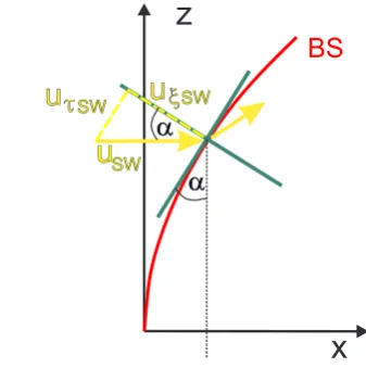
be determined. Consider the xz-plane; parametrization of the bow shock curve by introducing the angleα(z)(see Fig. C1) allows for the representation of the solar wind velocity’s and magnetic field’s component normal to the bow shock as

uξ,SW=cos(α(z)) uSW≈uSW, (C10)

Bξ,SW=sin(α(z)) BSW≈α(z) BSW, (C11)

and the tangential components as

uτ,SW=sin(α(z)) uSW≈α(z) uSW, (C12)

Bτ,SW=cos(α(z)) BSW≈BSW. (C13)

Here, Taylor expansion up to the first order inαwas used. Apparently, the solar wind’s normal velocity and tangential magnetic field remain approximately constant close to the stagnation streamline (small α), whereas the normal mag-netic field component and the tangential velocity vanish.

x

z

BS

u

u

_t

u

a

a

Fig. C1. Projection of the solar wind velocity vector with respect to

curvilinear bow shock coordinates.

Note that variations in tangential direction (of the compo-nents with respect to the shock’s surface), given by deriva-tives with respect to α, require the opposite. As a conse-quence of the negligible normal magnetic field component, the Rankine–Hugoniot relations require continuity of the tan-gential velocity components of the solar wind across the bow shock (Siscoe, 1983):

uτ,BS,1=uSW·τBS,1=

2cBS,yuSWy

ny

, (C14)

uτ,BS,2=uSW·τBS,2=

2cBS,zuSWz

nynyz

. (C15)

Relation (C3) holds for a normal solar wind velocity with a tangential magnetic field. Because the magnetic field is nearly tangential close to the subsolar point, we extent the scope of this relation to the vicinity of the stagnation stream-line using the normal component of the velocities:

uSW·ξBS=guu(x˜=0, y, z)·ξBS. (C16)

With the solar wind flowing along the x-axis, Eqs. (C3), (C5), and (C9) yield

uξ,BS=

ux0(x˜=0)

nyz

. (C17)

Substituting the coefficients (C14), (C15), and (C17) and the coordinate vectorsξBS,τBS,1, andτBS,2in Eq. (C9), the

ini-tial velocity writes

u(x˜=0, y, z)=1u

nyz

uSW

nyz

1u−1,2cBS,yy,2cBS,zz

T

,

(C18) where1u=uSW−ux0(x˜=0). Expanding this relation into

streamline and equating coefficients with the ansatz (16)– (18) yields values for the coefficient functions that can be expressed as

ul i j(x˜=0)=fu(i, j )2i+jciBS,yc j

BS,z1u, (C19)

wherel∈ {x, y, z}, the indicesi andj label the coefficient functions as in the ansatz (16)–(18), andfu(i, j )denotes the sign-function:

fu(i, j )=

+1, i+j ∈ {1}

−1, i+j ∈ {2,3}. (C20) The magnetic field can be treated in a similar manner. Its postshock values are expressed as follows:

B(x˜=0, y, z)=Bξ,BSξBS+ X

i=1,2

Bτ,BS,iτBS,i. (C21) The normal component of the magnetic field is always con-tinuous through the bow shock, which yields

Bξ,BS=

−2BSWcBS,zz

nyz

. (C22)

Similar to the velocity calculation, we extend the validity of relation (C4) to the vicinity of the stagnation streamline:

BSW·τBS,i=gBB(x˜=0, y, z)·τBS,i, (C23) wherei∈ {1,2}. With the solar wind magnetic field along the z-axis, Eqs. (C4), (C6), (C8), and (C21) give one

Bτ,BS,1=0, (C24)

Bτ,BS,2=

Bz0(0)ny

uz

. (C25)

Finally, the postshock magnetic field is

B(x˜=0, y, z)=1B

n2 yz

2cBS,zz,−4cBS,ycBS,zy z, (C26)

Bz0(0)+4BSWc_BS,y2 y2+4BSWc_BS,z2 z2

1B

!T

,

where1B=BSW−Bz0(x˜=0). The field boundary values

on the stagnation streamline result from the derivatives of Eqs. (13)–(15) at (x˜=0, y=0, z=0) and of Eq. (C26):

Bl i j(0)=fB(i, j )2i+jcBS,yi c j

BS,z1B, (C27)

in which

fB(i, j )=

+1, i+j∈ {1,2}

−1, i+j∈ {3} , (C28)

wherel∈ {x, y, z}, and the indicesi andj label the coeffi-cient functions as in the ansatz (13)–(15).

Note that Eqs. (C19) and (C27) satisfy the Frozen-in con-servation Eq. (29) as expected. Under the assumptions ap-plied in these calculations, the boundary values for the den-sity and pressure coefficientsρ20,ρ02,p20, andp02are zero.

Appendix D

Zeroth-order approach

To obtain a first approach to the physics and the correspond-ing solutions of the MHD equations, the zeroth-order ap-proach with its Eqs. (20)–(23) is solved analytically. The co-efficient functions of the first order are set to constant post-shock values:Bx01=Bx01(x˜=0),uy10=uy10(x˜=0), and

uz01=uz01(x˜=0). The latter two expressions are called

di-vergence parameters describing the amount of flow diversion in the respective tangential direction. The system is solved for arbitrary solar wind conditions.

D1 General solutions

For simplification, we neglect magnetic shear, meaning mag-netic fields in z-direction only, and consequentlyBx01(x˜=

0)=0. The shock front decelerates and compresses the flow; dynamic pressure is converted into gas and magnetic pres-sure. Most often, in the magnetosheath, the dynamic pressure term in the momentum equation of zeroth order (22) can be neglected (the minor effects of the dynamic pressure are dis-cussed in Sect. 4.1). This yields

k ργ₀0+ 1

µ0

Bz0Bz00 =0, (D1)

for which the zeroth-order adiabatic law (Eq. 23) has been used. Integration gives

k ργ₀+ B

2 z0

2µ0

=kρ0(0)γ+

Bz0(0)2

2µ0

, (D2)

with the integration constant on the right side to be deter-mined at the bow shock. The zeroth-order continuity Eq. (20) and the zeroth-order Frozen-in theorem (21) can be written as

u0_x0= −(uy10+uz01)+, (D3)

u0_x0= −uy10−δ, (D4)

where= −ux0∂xρ0/ρ0andδ=ux0∂xBz0/Bz0. The

north-ward magnetic field and the density are positive functions. Furthermore, andδ are always positive because the mag-netic field increases in the magnetosheath, corresponding to a decreasing density as given by Eq. (D1). The positive

andδ, and Eqs. (D3) and (D4) also provide lower and upper bounds for the velocity decrease:

−(uy10+uz01) < u0x0<−uy10. (D5)

Expanding the velocity inx˜around the bow shock reads

ux0=ux0(0)+ ∞ X

i=1

Note that the argument of the coefficient functions is with re-spect tox˜, soux0(0)=ux0(x˜=0)and is not explicitly noted

further. First, we take only the first order inx˜into account:

ux0=ux0(0)+ax.˜ (D7)

Herea=a1for the expansion coefficient was used. An

up-per bound for the error of the linear approach can be esti-mated using Eq. (D5). However, an almost-linear decrease of the velocity along the stagnation streamline is also in accord with global MHD simulation results by, e.g., Wu (1992) or Wang et al. (2004), and also agrees with the observations dis-played in Fig. 1. Note that in the hydrodynamic limit the den-sity is constant (incompressible fluid) because of Eq. (D1). This leads to=0 with the consequence of a linear veloc-ity decrease witha= −uy10−uz01. Substituting the velocity

ansatz (D7) in the zeroth-order continuity Eq. (20) and the Frozen-in theorem (21) gives

ρ0=ρ0(0)

_u

x0

ux0(0) −

uy10+uz01+a a

, (D8)

Bz0=Bz0(0)

_u

x0

ux0(0) −

uy10+a a

. (D9)

An expression for the expansion parameterais obtained by substituting the results forρ0andBz0in the simplified

mo-mentum equation (D2):

k



ρ0(0)

_u

x0

ux0(0)

−uy10+uz01+a

a



 γ

(D10)

+ 1 2µ0



Bz0(0)

_u

x0

ux0(0) −

uy10+a a



 2

=kρ0(0)γ+

Bz0(0)2

2µ0

.

To solve this equation, both sides are expanded into Taylor series aroundx˜=0. Equating coefficients of the lowest non-vanishing order yields

a= −uy10−uz01 

1− 1 1+γ

2 p0(0) pmag(0)



. (D11)

Herepmag(0)=Bz02(0)/2µ0denotes the postshock magnetic

pressure andγ=5/3 the ratio of specific heats.

This result is used to obtain an expression for the mag-netosheath thickness xMS. The magnetopause is defined

by a vanishing flow velocity on the stagnation streamline (ux(xMS)=0). Equation (D7) thus yields

xMS=

ux0(0)

a . (D12)

After substitution of Eq. (D11), we obtain

xMS=

−ux0(0)

uy10+mBSuz01

, (D13)

with

mBS=1−

1 1+γ

2 p0(0) pmag(0)

. (D14)

The parametermBSis a measure for the solar wind

magneti-zation. For the unmagnetized solar wind, we obtainmBS=1.

Note that the magnetosheath expression results from ideal MHD equations, neglecting magnetic shear (Bx01(0)=0)

and the dynamic pressure terms, and using a series ansatz for the velocity (u=(ux0(0)+ax, u˜ y01(0), uz10(0))T).

Higher-order contributions of the velocity to the magne-tosheath thickness can also be obtained. For a second-order ansatz for the velocity in x˜-direction, similar calculations yield the second-order expansion coefficient:

a2=

2γ2pmag(0) p0(0) pmag(0)+p0(0)u2_z01

2pmag(0)+γp0(0)3ux0(0)

. (D15)

In the limit p0(0) >> pmag(0) the expression is

approxi-mated by:

a2≈2γ

pmag(0)

p0(0)

u2_z01

ux0(0)

. (D16)

Consistently,a2vanishes in the limit of hydrodynamics (i.e.,

pmag(0)=0) and a linear velocity decrease remains.

D2 Boundary conditions

The divergence parameters are set to their bow shock values, which are given by Eq. (C19):

uy10=2cBS,y1u, (D17)

uz01=2cBS,z1u. (D18)

The geometry parameterscBS,y andcBS,z need to be

deter-mined.

The dynamic pressure of the solar wind is completely con-verted into gas and magnetic pressure in the magnetosheath. However, pressure is not a conserved quantity and, thus, the solar wind pressure differs by a factorK from the magne-topause pressure on the stagnation streamline:

K ρSWu2SW=ptot,MP, (D19)

where the total magnetopause pressureptot,MP is given by

The pressure balance equation above is valid at the stag-nation point (x˜=xMS, y=0, z=0) only. In its vicinity, only

the velocity component normal to the local magnetopause is important. The dynamic pressure with respect to the magne-topause normal (Eq. 41) thus reads

pdyn,ξ=ρSWu2SW,ξ=ρ

u2_SW

n2_MP. (D20)

This expression holds for both the y- and z-directions. Here-with, the pressure equilibrium writes

K pdyn,ξ=ptot,MP, (D21)

where Eq. (48) was used andf =2.44. Note that by setting

K=1 the pressure relation becomes equivalent to the one used by Mead and Beard (1964).

Using the magnetopause parametrization (10), the Earth’s dipole field (Eqs. 6–8), the magnetopause normal vector (Eq. 41), and the magnetospheric pressure (Eq. 48) in the xy-plane yield

ptot,MP,xy=

f2

2µ0

M2

(1xMP−cMP,yy2)2+y23

. (D22)

Substitutingptot,MPin Eq. (D19) by this pressure relation, the

magnetopause distance1xMPat the stagnation point (y=0)

is obtained, given by the well-know expression (e.g., Pu-dovkin et al., 1998)

1xMP=

f2M2

2µ0KρSWu2SW !1₆

. (D23)

The geomagnetic dipole moment is given by M=8× 1015Tm3. The general pressure balance (D21) along with Eqs. (D20) and (D22) is solved using Taylor expansion with respect to y around the stagnation point up to the second order. Equating coefficients allows for determination of the magnetopause curvature:

cMP,y=

−3+ √

21 41xMP

≈ 0.4

1xMP

. (D24)

This expression now enables us to estimate the parabolic co-efficientcBS,y, which we need to know for an estimate of the

postshock divergence. We assume the same functional ex-pression for the curvature of the bow shock as derived for the magnetopause above:

cBS,y=

0.4

1xBS

= 0.4

1xMP+xMS

. (D25)

The divergence parameter uy10 is now calculated with

Eq. (D17):

uy10=0.8

uSW−ux0(0)

1xMP+xMS

, (D26)

where1u=uSW−ux0(0)was used, as defined above.

The velocity divergence within the xz-plane remains to be determined. Using Eq. (48) to describe the magnetospheric pressure within the xz-plane leads to

ptot,MP,xz=

2z2−1x2−6cMP,z1x z2 2

1+4c2_MP,zz2 _1x2_+z25

f2M2

2µ0

, (D27)

which yields

cMP,z=

1 21xMP

. (D28)

Assuming, again, the same functional expression for the bow shock curvature gives

cBS,z=

1 21xBS

= 1

2(1xMP+xMS)

, (D29)

and using Eq. (D18) the divergence parameteruz01reads

uz01=

uSW−ux0(0)

1xMP+xMS

. (D30)

Altogether, after some tedious calculations, Eqs. (D26) and (D30) provide suitable estimates for flow divergence just af-ter the bow shock. The numerator is deaf-termined by the veloc-ity jump across the bow shock, and the denominator by the bow shock’s distance to the Earth’s center. The ratio of both divergence parameters is

uy10=

4

5uz01. (D31)

This equation describes the asymmetry of the divergence in y- and z-direction in the approach discussed.

The expressions for the divergence still depend on the magnetosheath thickness. With Eqs. (C3), (D13), (D26), and (D30) we get

xMS=

1xMP

4

5+mBS

(gu−1)−1

. (D32)

This relation for the magnetosheath thickness depends on the solar wind conditions only. The velocity jump at the bow shockgu(Eq. C3), the magnetopause distance form the Earth’s center1xMP(Eq. D23), and the solar wind

magneti-zationmBS(Eq. D14) are explicit functions of the solar wind

parameters. Equations (C1)–(C4) are used to refer the bow shock conditionsρ0(0), p0(0),Bz0(0), andux0(0)back to

solar wind conditions. Hence, Eqs. (D26) and (D30) can also be written as explicit functions of these solar wind parame-ters.

D3 Application