Modes of zonal mean temperature variability 20–100 km from the TIMED/SABER observations

Ann. Geophys., 32, 285–292, 2014 www.ann-geophys.net/32/285/2014/ doi:10.5194/angeo-32-285-2014

© Author(s) 2014. CC Attribution 3.0 License.

Annales

Geophysicae

Open Access

Modes of zonal mean temperature variability 20–100 km from the

TIMED/SABER observations

Y. Jiang, Z. Sheng, and H. Q. Shi

College of Meteorology and Oceanography, PLA University of Science and Technology, Nanjing, 211101, China Correspondence to: Z. Sheng ([email protected])

Received: 20 August 2013 – Revised: 29 December 2013 – Accepted: 10 February 2014 – Published: 27 March 2014

Abstract. In this study we investigate the spatial

variabil-ities of the zonal mean temperature (20–100 km) from the TIMED (Thermosphere, Ionosphere, Mesosphere, Energet-ics and DynamEnerget-ics)/SABER (Sounding of the Atmosphere using Broadband Emission Radiometry) satellite using the empirical orthogonal functions (EOFs). After removing the climatological annual mean, the first three EOFs are able to explain 87.0 % of temperature variabilities. The primary EOF represents 74.1 % of total anomalies and is dominated by the north–south contrast. Patterns in the second and third EOFs are related to the semiannual oscillations (SAO) and mesospheric temperature inversions (MTI), respectively. The quasi-biennial oscillation (QBO) component is also decom-posed into the seventh EOF with contributions of 1.2 %. Last, we use the first three modes and annual mean temperature to reconstruct the data. The result shows small differences are in low latitude, which increase with latitude in the middle stratosphere and upper mesosphere.

Keywords. Atmospheric composition and structure

(pres-sure, density, and temperature)

1 Introduction

The thermal structure is significant for researching variations and coupling in the stratosphere and mesosphere. But the comprehensive description is difficult with sparse observa-tions. Ground-based techniques, falling spheres and rocket grenades (She and von Zahn, 1998; Leblanc et al., 1998; She et al., 2000; Lübken and Mullemann, 2003; Chu et al., 2005) cover limited positions and cannot offer a global struc-ture. Instruments on satellites in the past, such as Nimbus 7 (Gille and Russell, 1984; Remsberg et al., 2004), SME (Clancy et al., 1994) and UARS (Wu et al., 2003; Leblanc

and Hauchecorne, 1997; Shepherd et al., 2004; Ortland et al., 1998), were neither covering all local times nor high in res-olution. However, most shortcomings of previous measure-ments are overcome by the Sounding of the Atmosphere us-ing Broadband Emission Radiometry (SABER) instrument on the TIMED (Thermosphere, Ionosphere, Mesosphere, En-ergetics and Dynamics) satellite. With the data of high verti-cal resolution and global coverage, Huang et al. (2006) and Xu et al. (2007a, b) analyzed 2 years and 5 years of SABER temperature, respectively. In this paper we attempt to derive dominant spatial distributions of the given data sets by de-composing SABER temperature using the empirical orthog-onal functions (EOFs).

EOFs are also called the conventional principal component analysis (PCA), which estimates the principal spatial and temporal variations depicted by regular observations. This method, usually taking the approach of the sample covari-ance, has been used in various fields such as ionospheric physics in Sun et al. (1998), the sea surface temperature (SST) in Chu et al. (1997, 1998) and nitric oxide in the lower thermosphere Marsh (2004). However, it is the first time this technique is applied to decompose temperature between 20 and 100 km with SABER data.

2 Data set

middle mesosphere in the 1.07 version temperature. From 85 to 100 km, SABER data and sodium lidar are in quite good agreement (Xu et al., 2006). Errors are about±1–2 K below 95 km and±4 K at 100 km and increase to±3 K at 80 km and

±8 K at 90 km when there are strong temperature inversion layers (García-Comas et al., 2008).

It almost takes 60 days for the SABER measurements to cover all local times. To reduce tides and planetary wave effects, two months in a year are grouped as JF (January– February), MA (March–April), MJ (May–June), JA (July– August), SO (September–October), and ND (November– December). The stationary planetary waves and the non-migrating tides could be excluded by averaging tempera-ture along longitude for each day (Xu et al., 2007a). As for migrating tides, Lieberman (1991) and Oberheide and Gu-sev (2002) determined them by subtracting ascending node observations from descending ones, or vice versa. Therefore, adding ascending and descending node data cancel out most migrating tides. For planetary waves with multi-periods, two months are long enough to attenuate them by zonal averag-ing. Since the satellite covers latitudes poleward of 53◦ in one hemisphere in a yaw cycle, only data within the regions of 52.5◦S–52.5◦N are studied to avoid data gaps. Then, each bimonthly data are averaged in bins of 5◦in latitude and 1 km in altitude. The altitude range is 20–100 km. We use 9 year data sets from 2003 to 2011 in this paper.

3 Methodology

The bimonthly mean temperature is denoted by

T (xi,yj, τn, tm), where (xi,yj) denotes horizontal grids (i=1,2, . . . ,21;j =1,2, . . . ,81),τn yearly sequence, and

tm=1,2, . . . ,6, the bimonthly sequence. The climatological annual mean is

T (xi,yj)= 1 54

6 X

m=1 9 X

n=1

T (xi,yj, τn, tm), (1)

the data anomalies are expressed as

b

T (xi,yj, τn, tm)=T (xi,yj, τn, tm)−T (xi,yj). (2) Then the Tb is rearranged into a two-dimension matrix, bT(r, p),r=21×81, andp=6×9.ris the number of grids.

pis the length of time sequence. The temperature anomalies are decomposed as follows using the singular value decom-position (SVD) algorithm (Wilks, 2006):

bT(r, p)= X

v

PC(v)(p)×EOF(v)(r), (3)

whereP C(v)(p)is the time-dependent coefficient of thevth EOF, or EOF(v)(r).

400

401

Figure 1. Percent variances for the first ten mode. 402

403

404

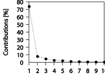
Fig. 1. Percent variances for the first ten modes.

To determine the degeneracy of EOFs, North et al. (1982) concluded a rule of thumb:

δλv=λv(2/N )1/2, (4)

λv−λv+1≥δλv, (5) whereNis an effective sample size of 54 here. The degener-acy of EOFs does not occur if sampling errorsδλvin eigen-values are smaller than spacingλv−λv+1. In other words, a sample EOF should not represent a trusted EOF if the sam-pling error is close to the spacing.

The Morlet wavelet is performed on the PCs (princi-ple components)to analyze periods. First, wavelet coeffi-cients are calculated by changing the wavelet scale along the time series. Then we get the wavelet power spectrum by squaring the wavelet transform at each period. Torrence and Compo (1998) have described this in detail.

4 Results and discussion

Figure 1 shows the percent variances for first ten EOF series. Contributions of sample EOFs and ratios of spacing to sam-pling error in eigenvalues for the first ten orders are listed in Table 1. Most variances are from the first EOF. The ratios in-dicate that the first three EOFs contain small sampling errors and thus represent meaningful climatological fields. Degen-eracy occurs for the fourth EOF because the sampling error is larger than the spacing. So we essentially analyze the first three leading EOFs.

Table 1. Contributions of first ten order EOFs and ratiosδλv/(λv−λv+1).

Order (v) 1 2 3 4 5 6 7 8 9 10

Contributions (%) 74.1 8.1 4.8 2.9 2.4 1.4 1.2 0.8 0.7 0.5

δλv/(λv−λv+1) 0.22 0.48 0.48 1.05 0.46 1.42 0.63 1.09 0.67 1.57

405

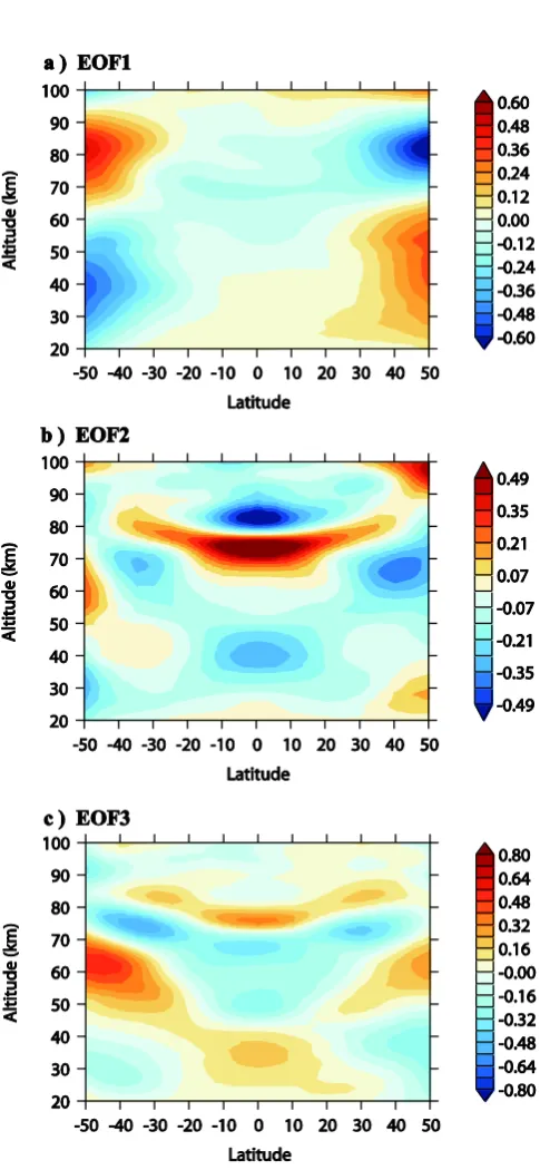
Figure 2. (a-c) The first 3 EOFs of the SABER data anomalies. 406 Fig. 2. (a–c) The first three EOFs of the SABER data anomalies.

The EOF(1)shows an apparent interhemispheric asymme-try: anomalies in the southern upper stratosphere and north-ern upper mesosphere are larger than those at the other hemi-sphere. Figure 4a presents that the PC(1)has an annual vari-ation (Fig. 4a), indicating that annual oscillvari-ation (AO) is the main reason. The EOF(1) shares a similar pattern with the AO distribution from Xu et al. (2007a). The warmest and coldest positions at high latitudes are where largest ampli-tudes of AO exist regardless of signs of PCs. Contributions of 74.1 % from the north–south contrast pattern are in concert with relative amplitude of over 90 % in some regions for AO compared to other periodic variations (Xu et al., 2007a). The strongest AO at high latitudes is also found by Shepherd et al. (2004) using the Wind Imaging Interferometer (WINDII) on the Upper Atmosphere Research Satellite (UARS) and nightly temperatures from various ground-based hydroxyl airglow observations.

In the second EOF, the most remarkable patterns are strong, warm anomalies in the tropical mesosphere from 70 to 80 km and a mirror image above it when PC(2) is pos-itive. This contrast indicates that temperature anomalies in these two areas are negatively correlated. A plausible expla-nation are the semiannual oscillations (SAO). According to Xu et al. (2007a), in the tropical regions, amplitudes of SAO are minimum at∼25–50 km and∼80–90 km and are max-imum at∼65–80 km in January and July. When PC is posi-tive, three regions with extreme temperature values centered at around 40, 75 and 85 km, which is in good agreement with altitudes of amplitude peaks of the SAO. In spring and au-tumn, amplitudes of the SAO at 80–90 km increase to max-imum (Xu et al., 2007a), larger than those at 65–80 km, so the warm regions in Fig. 2b should turn to cold and thus PC should become negative, which is consistent with calculated PCs.

407

408

Figure 3. Time series of first three PCs in the period of 2003-2011. 409

410

Fig. 3. Time series of first three PCs in the period of 2003–2011.

Although the PC(3)shares the same period and partly sim-ilar patterns with the PC(2), mechanisms underlying EOF(3) and EOF(2)are not the same. The EOF(2)is dominated by the SAO, which is strongest in the tropical upper mesosphere af-ter the AO has been extracted. The third EOF is controlled by the lower mesospheric temperature inversions (MTIs) (Meri-wether and Mlynczak, 1995; Meri(Meri-wether and Gardner, 2000; Meriwether and Gerrard, 2004) in the mesosphere. Typically, temperature declines above the stratopause until it reaches the mesopause. When MTIs occur, temperature abruptly in-creases by more than 20 K, which is warmer than the temper-ature below it. The minimum tempertemper-ature under the inversed temperature is referred to as the secondary minimum (SM). Thus, warm/cold anomalies form in the tropical mesosphere. The MTI is strong at equinox but rather weak in winter. The time series of PC(3) also exhibit a semiannual cycle, which agrees with ground-based observations at Gadanki (13.5◦_N, 79.2◦_{E) by Venkat Ratnam et al. (2010). In the subtropical} mesosphere, mirror patterns weaken and elevate to higher lat-itudes. Das et al. (2011) obtain the mean MTI and SM alti-tudes of 87 and 80 km over Taiwan (21–27◦N, 119–123◦E), which is in good agreement with our results.

The MTI is not only being observed in the tropical meso-sphere but also in the midlatitude mesomeso-sphere. Hauchecorne et al. (1987) reported variations of the MTI using two 411

412

Figure 4. The global power spectrum for (a) PC(1), (b) PC(2) and (c) PC(3). The dotted 413

line is the 95% confidence level. 414

415

Fig. 4. The global power spectrum for (a) PC(1), (b) PC(2) and (c) PC(3). The dotted line is the 95 % confidence level.

Rayleigh lidars located at about 46◦N. They found its al-titude is of 55–72 km in winter and 70–83 km in summer. The occurrence frequency for the MTI is higher at solstices than at equinoxes. Further reports of the MTI are from the Rayleigh lidar at York University (43◦N, 79◦W), which said that the MTI occurred below 70 km during winter and above that height in summer with occurrence of 90 % (Whiteway et al., 1995). Liu and Meriwether (2004) observed verti-cal wave structure during a MTI and found large projected background wind can generate observed event numerically. They attributed the MTI to a developing frontal system in the tropopause region. These observations coincide with the cold/warm regions in the third EOF. When MTI occurs be-tween 50 and 70 km at midlatitudes, the temperature is higher than those above it, then temperatures in the two areas are an-ticorrelated. As the inversion occurs above 70 km, this con-trasting pattern exists. Since the occurrence of the MTI in the lower altitude is higher than those above 70 km, the warm re-gions are stronger and wider than the cold area.

416

Figure 5. The seventh EOF (a) and the power spectrum of the PC(7) (b). The dotted 417

line denotes the 95% confidence level. 418

419

Fig. 5. The seventh EOF (a) and the power spectrum of the PC(7) (b). The dotted line denotes the 95 % confidence level.

An interesting phenomenon for our second and third EOF decomposition is its association with changes in zonal mean temperature between February 2002 and December 2006 by Xu et al. (2007a, Fig. 14). Although their results are trends between 2002 and 2006, temperature changes exhibit cor-relation in the latitude–altitude cross section. According to their results, during the 5 years, temperature increased in three different regions: one in the tropical stratosphere from 30 to 40 km and two in the midlatitude mesosphere from 50 to 70 km. Among regions where temperature declined, the maximum of more than 5 K was found at the midlatitude mesosphere between 80 and 95 km. Positions of decreased and increased temperature are in agreement with warm re-gions below 70 km and cold rere-gions in Fig. 2, respectively.

The strong, warm region in the second EOF is where tem-perature increased from 2002 to 2006. The negative corre-lation between low latitude (equatorward of 20◦) and high latitude (poleward of 20◦_{) in the stratosphere in Fig. 2b and c} is found in temperature changes over a timescale of 5 years. Another case in the mesosphere is that lidar observations at the Haute Provence (44◦N) show positive and negative re-sponses to the solar flux variations up to 70 and above 80 km, respectively. All of those resemblances between the tempo-ral distribution and temperature changes are not coincidence. These relations provide an insight into causes for the tem-perature trend. Actually, our results are in agreement with arguments of Beig (2003). It is the dynamics that change the solar response in the mesosphere at different latitudes.

5 Reconstruction

The first three EOF modes and PCs and zonally mean tem-peratures are used to reconstruct the temperature in the range of 20–100 km from 2003 to 2011. Figure 6 shows the six zon-ally bimonthly temperatures. The left column is real temper-ature and the right one is reconstructed data for 2003. Results show that the first three EOFs could explain major character-istics in the stratosphere and mesosphere in different months. The best agreements are found in low latitudes. Large biases are seen in midlatitudes, especially at around 50–80 km.

420

Fig. 6. The real (left column) and reconstructed (right column)

424

425

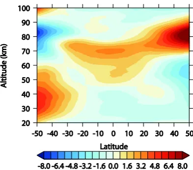
Figure 7. Percentage of relative differences using 9-year data. 426

427

Fig. 7. Percentage of relative differences using 9 year data.

Figure 7 exhibits the percentage of relative differences (100 %× (reconstructed data−observed data)/observed data) with 9 year data. Temperature in the midlatitude south-ern stratosphere and in the upper northsouth-ern mesosphere is warmer with a maximum of more than 5 and 9 %, respec-tively. Temperature in the low latitudes in the range of 50– 80 km shows warm biases with a maximum of∼3 %. Neg-ative biases are in the tropical and north hemispheric strato-sphere and southern Southern Hemistrato-sphere. The distribution percentage is similar to that of EOF(1)and the PC(1)is posi-tive, suggesting that the AO is not fully extracted in the first mode.

Figure 8 shows temporal variations of temperature relative differences percentage between the constructed data and ob-servations at eight points from 2003 to 2012. The best agree-ment is found at the Equator at the height of 70 km with a mean difference of−0.6 K. In the stratosphere, cold biases are in the Northern Hemisphere and warm biases are in the Southern Hemisphere. This situation reverses in the meso-sphere because of the opposite transformation of tempera-ture between stratosphere and mesosphere. The largest mean difference at 80 km is 18.5 K in the Northern Hemisphere. Obvious biases beyond low latitudes indicate that some sig-nificant variations might be in the fourth or higher modes, which do not play an important role at low latitudes.

6 Summary

The SABER temperature from 2003 to 2011 is successfully decomposed into dominant modes with the EOF method. For the first time, the spatial coherence of anomalies in the range of 20–100 km is exhibited, revealing important transi-tion from the low stratosphere to upper mesosphere. Domi-nant modes in the first three EOFs are attributed to the AO, SAO and MTI. The EOF(7) is characterized by the QBO with a contribution of 1.2 %. Similar patterns found in tem-perature changes over a long time and warm/cold regions

Fig. 8. Percentage of temperature relative difference at different

al-titude and laal-titude.

in the second and third modes suggest that solar response of mesospheric temperature is mainly affected by dynamics. The constructed data using the first three modes represent well the original measurements. The temperature differences increase with latitude, which will be investigated in further research. Large differences are due to the AO.

Acknowledgements. We thank the SABER team for providing data

through the FTP site. The work was partly supported by the Na-tional Natural Science Foundation of China (Grant no. 41105013, 41375028), the National Natural Science Foundation of Jiangsu, China (Grant no. BK2011122), the Jiangsu Key Laboratory of Me-teorological Observation and Information Processing scientific re-search fund, China (Grant no. KDXS1205).

Topical Editor C. Jacobi thanks two anonymous referees for their help in evaluating this paper.

References

Beig, G.: Review of mesospheric temperature trends, Rev. Geo-phys., 41, 1015, doi:10.1029/2002rg000121, 2003.

Chu, P. C., Lu, S., and Chen, Y.: Temporal and spatial variabilities of the South China Sea surface temperature anomaly, J. Geophys. Res., 102, 20937–20955, 1997.

Chu, P. C., Chen, Y., and Lu, S.: Temporal and Spatial Variabilities of Japan Sea Surface Temperature and Atmospheric Forcings, J. Oceanogr., 54, 273–284, 1998.

Chu, X., Gardner, C. S., and Franke, S. J.: Nocturnal thermal struc-ture of the mesosphere and lower thermosphere region at Maui, Hawaii (20.7◦N), and Starfire Optical Range, New Mexico (35◦ N), J. Geophys. Res., 110, D09S03, doi:10.1029/2004JD004891, 2005.

Clancy, R. T., Rusch, D. W., and Callan, M. T.: Temperature minima in the average thermal structure of the middle atmosphere (70– 80 km) from analysis of 40 to 92 km SME global temperature profiles, J. Geophys. Res., 99, 19001–19020, 1994.

Das, U. and Pan, C. J.: The temperature structure of the mesosphere over Taiwan and comparison with other latitudes, J. Geophys. Res., 116, D00P06, doi:10.1029/2010JD015034, 2011. García-Comas, M., López-Puertas, M., Marshall, B. T.,

Gille, J. C. and Russell III, J. M.: The limb infrared monitor of the stratosphere (LIMS): experiment description, performance and results, J. Geophys Res., 89, 5125–5140, 1984.

Hauchecorne, A., Chanin, M. L., and Wilson, R.: Mesospheric tem-perature inversion and gravity wave breaking, Geophys. Res. Lett., 14, 933–936, doi:10.1029/GL014i009p00933, 1987. Huang, F. T., Mayr, H. G., Reber, C. A., Russell, J. M., M Mlynczak,

and Mengel, J. G.: Stratospheric and mesospheric tempera-ture variations for the quasi-biennial and semiannual (QBO and SAO) oscillations based on measurements from SABER (TIMED) and MLS (UARS), Ann. Geophys., 24, 2131–2149, doi:10.5194/angeo-24-2131-2006, 2006.

Leblanc, T. and Hauchecorne, A.: Recent observations of meso-spheric temperature inversions, J. Geophys. Res., 102, 19471– 19482, 1997.

Leblanc, T., McDermid, I. S., Keckhut, P., Hauchecorne, A., She, C. Y., and Krueger, D. A.: Temperature climatology of the middle atmosphere from long-term lidar measurements at mid-dle and low latitudes, J. Geophys. Res., 103, 17191–17204, doi:10.1029/98JD01347, 1998.

Lieberman, R. S.: Nonmigrating diurnal tides in the equa-torial middle atmosphere, J. Atmos. Sci., 48, 1112–1123, doi:10.1175/1520-0469(1991)048<1112:NDTITE>2.0.CO;2, 1991.

Liu, H.-L. and Meriwether, J. W.: Analysis of a temperature in-version event in the lower mesosphere, J. Geophys. Res., 109, D02S07, doi:10.1029/2002JD003026, 2004.

Lübken, F. J. and Mullemann, A.: First in situ temperature measure-ments in the summer mesosphere at very high latitudes (78◦N), J. Geophys. Res., 108, 8448, doi:10.1029/2002JD002414, 2003. Marsh, D. R.: Empirical model of nitric oxide in the lower thermosphere, J. Geophys. Res., 109, A07301, doi:10.1029/2003ja010199, 2004.

Meriwether, J. W. and Gardner, C. S.: A review of the mesosphere inversion layer phenomenon, J. Geophys. Res., 105, 12405– 12416, doi:10.1029/2000JD900163, 2000.

Meriwether, J. W. and Gerrard, A. J.: Mesosphere inversion layers and stratosphere temperature enhancements, Rev. Geophys., 42, RG3003, doi:10.1029/2003RG000133, 2004.

Meriwether, J. W. and Mlynczak, M. G.: Is chemical heating a major cause of the mesosphere inversion layer?, J. Geophys. Res., 100, 1379–1387, doi:10.1029/94JD01736, 1995.

Mertens, C. J., Mlynczak, M. G., Lopez-Puertas, M., Wintersteiner, P. P., Picard, R. H., Winick, J. R., Gordley, L. L., and Russell III, J. M.: Retrieval of mesospheric and lower thermospheric kinetic temperature from measurements of CO215 mm Earth limb

emis-sion under non-LTE conditions, Geophys. Res. Lett., 28, 1391– 1394, doi:10.1029/2000GL012189, 2001.

Mertens, C. J., Schmidlin, F. J., Goldberg, R. A., Remsberg, E. E., Pesnell, W. D., Russell, J. M., Mlynczak, Martin, G., López-Puertas, M., Wintersteiner, P. P., and Picard, R. H.: SABER observations of mesospheric temperatures and compar-isons with falling sphere measurements taken during the 2002 summer MaCWAVE campaign, Geophys. Res. Lett., 31, L03105, doi:10.1029/2003GL018605, 2004.

North, G. R., Bell, T. L., Cahalan, R. F., and Moeng, F. J.: Sampling errors in the estimation of empirical orthogonal functions, Mon. Weather Rev., 110, 699–706, 1982.

Oberheide, J. and Gusev, O. A.: Observation of migrating and non-migrating diurnal tides in the equatorial lower thermosphere, Geophys. Res. Lett., 29, 2167, doi:10.1029/2002GL016213, 2002.

Ortland, D. A., Hays, P. B., Skinner, W. R., and Yee, J.-H.: Re-mote sensing of mesospheric temperature and O2(1S) band vol-ume emission rates with the high-resolution Doppler imager, J. Geophys. Res., 103, 1821–1836, 1998.

Remsberg, E. E., Gordley, L. L., Marshall, B. T., Thompson, R. E., Burton, J., Bhatt, P., Harvey, V. L., Lingenfelser, G., and Natara-jan, M.: The Nimbus 7 LIMS version 6 radiance conditioning and temperature retrieval methods and results, J. Quant. Spec-trosc. Radiat. Transfer, 86, 395–424, 2004.

Remsberg, E. E., Marshall, B. T., Garcia-Comas, M., Krueger, D., Lingenfelser, G. S., Martin-Torres, J., Mlynczak, M. G., Russell III, J. M., Smith, A. K., and Zhao, Y.: Assessment of the qual-ity of the Version 1.07 temperature-versus-pressure profiles of the middle atmosphere from TIMED/SABER, J. Geophys. Res., 113, D17101, doi:10.1029/2008JD010013, 2008.

She, C. Y. and von Zahn, U.: Concept of a two-level mesopause: Support through new lidar observations, J. Geophys. Res., 103, 5855–5863, doi:10.1029/97JD03450, 1998.

She, C. Y., Chen, S., Hu, Z., Sherman, J., Vance, J. D., Va-soli, V., White, M. A., Yu, J., and Krueger, D. A.: Eight-year climatology of nocturnal temperature and sodium den-sity in the mesopause region (80 to 105 km) over Fort Collins, Co (41◦ N, 105◦ W), Geophys. Res. Lett., 27, 3289–3292, doi:10.1029/2000GL003825, 2000.

Shepherd, M. G., Evans, W. F. J., Hernandez, G., Offermann, D., and Takahashi, H.: Global variability of mesospheric tempera-ture: Mean temperature field, J. Geophys. Res., 109, D24117, doi:10.1029/2004JD005054, 2004.

Sun, W., Xu, W.-Y., and Akasofu, S.-I.: Mathematical separation of directly driven and unloading components in the ionospheric equivalent currents during substorms, J. Geophys. Res., 103, 11695–11700, 1998.

Torrence, C. and Compo, G. P.: A practical guide to wavelet analy-sis, Bull. Am. Meteorol. Soc., 79, 61–78, 1998.

Venkat Ratnam, M., Patra, A. K., and Krishna Murthy B. V.: Trop-ical mesopause: Is it always close to 100 km?, J. Geophys. Res., 115, D06106, doi:10.1029/2009JD012531, 2010.

Whiteway, J. A., Carswell, A. I., and Word, W. E.: Mesospheric temperature inversions with overlaying nearly adiabatic lapse rate: An indication of a well-mixed turbulent layer, Geophys. Res. Lett., 22, 1201–1204, 1995.

Wilks, D. S.: Statistical Methods in the Atmospheric Sciences, 2nd Edn., Academic Press, Amsterdam, 2006.

Wu, D. L., Read, W. G., Shippony, Z., Leblanc, T., Duck, T. J., Ortland, D. A., Sica, R. J., Argall, P. S., A Oberheide, J., and Hauchecorne, A.: Mesospheric temperature from UARS MLS: retrieval and validation, J. Atmos. Solar-Terr. Phys., 65, 245–267, 2003.

Xu, J., Smith, A. K., Yuan, W., Liu, H.-L., Wu, Q., Mlynczak, M. G., and Russell III, J. M.: Global structure and long-term variations of zonal mean temperature observed by TIMED/SABER, J. Geo-phys. Res., 112, D24106, doi:10.1029/2007JD008546, 2007a.