Volume 7, Number 3, pp. 1–8. http://www.scpe.org c 2006 SWPS
EMPIRICAL PARALLEL PERFORMANCE PREDICTION FROM SEMANTICS-BASED PROFILING
NORMAN SCAIFE∗, GREG MICHAELSON†, AND SUSUMU HORIGUCHI‡
Abstract. The PMLS parallelizing compiler for Standard ML is based upon the automatic instantiation of algorithmic skeletons at sites of higher order function (HOF) use. Rather than mechanically replacing HOFs with skeletons, which in general leads to poor parallel performance, PMLS seeks to predict run-time parallel behaviour to optimise skeleton use.
Static extraction of analytic cost models from programs is undecidable, and practical heuristic approaches are intractable. In contrast, PMLS utilises a hybrid approach by combining static analytic cost models for skeletons with dynamic information gathered from the sequential instrumentation of HOF argument functions. Such instrumentation is provided by an implementation independent SML interpreter, based on the language’s Structural Operational Semantics (SOS), in the form of SOS rule counts. PMLS then tries to relate the rule counts to program execution times through numerical techniques.
This paper considers the design and implementation of the PMLS approach to parallel performance prediction. The formulation of a general rule count cost model as a set of over-determined linear equations is discussed, and their solution by single value decomposition, and by a genetic algorithm, are presented.
Key words. Parallel computation, profiling, performance prediction, program transformation.
1. Introduction. The optimal use of parallel computing resources depends on placing processes on pro-cessors to maximise the ratio of processing to communication, and to balance loads, to ensure that all propro-cessors are maximally and gainfully occupied. These two requirements are strongly related: moving processing from one processor to another in search of load balance changes inter-processor communication patterns. However, in the absence of standard methodologies or generic support tools, process/processor placement remains something of a black art, guided primarily by empirical experimentation on the target architecture. This can be a long and painstaking activity, which ties up scarce, costly parallel resources at the expense of other users. It would be most desirable to develop analytic techniques to guide process placement which do not depend on direct use of the target system.
Process placement is greatly simplified given accurate measures of individual process communication and processing behaviour. However, such measures, like most interesting properties of programs, are in general undecidable. The only alternative is to use to some mix of approximative techniques for static and dynamic analysis.
One approach is to focus on general patterns of processing with known behavioural characteristics. For parallel programming, Cole’s algorithmic skeletons [9] form a popular class of patterns, including the data parallel task farm and the binary tree structured divide and conquer. Here, simple analytic cost models have been constructed which give good predictions of parallel behaviour when instantiated appropriately [18].
Alas, this just pushes the problem down a level as it is still necessary to characterise the task specific behaviours that such patterns are to be populated with. For non-conditional and non-repetitive program fragments, precise measures may be found through static cost modeling. However, in the more general cases, either approximative static analyses or empirical measures must still be used.
Static methods such as computational complexity analysis [12] or microanalysis [8] break down in the presence of conditional and repetitive constructs. Computational complexity analysis implementations are often limited to libraries of known instances in these cases. Microanalysis has similar limitations, requiring the solutions to sets of difference equations which, in turn, lack direct analytic solutions.
Dynamic measures may be based onsampling andcounting methods. Sampling is where the program is interrupted at regular intervals and a picture of where processing is concentrated can be built up. This has been used for Standard ML [4]. Counting is where passage through specific points in the program are recorded. Examples of this are used in the PUFF compiler [7] and the SkelML compiler [6].
∗LASMEA, Blaise Pascal University, Les Cezeaux, F-63177 Aubiere cedex, France,
†Department of Computing and Electrical Engineering, Heriot-Watt University, Riccarton, Edinburgh, EH14 4AS,
‡Department of Computer Science, Graduate School of Information Sciences, Tohoku University, Aobayama 6-3-09, SENDAI
980-8579, JAPAN, ([email protected]).
Whatever technique is used to cost a program, the final measure must be related back to an actual perfor-mance on the target architecture. Typically, both static and empirical measures give counts of features, such as the presence of known operations, or behaviours, such as the number of times a construct is carried out. The equivalent costs on the target architecture may be established in terms of individual CPU instructions, either by direct instrumentation or from manufacturer’s specifications. This approach gives accurate predictions from sequential profiling but is highly implementation dependent.
An alternative is to time representative programs on the target architecture and relate the times back to the modeled costs. This offers a high degree of implementation independence but requires well chosen exemplars and, like rule counting, is very dependent on the test data.
2. Background. The PMLS (Parallelising ML with Skeletons) compiler for Standard ML [14] translates instances of a small set of common higher-order functions (HOFs) into parallel implementations of algorithmic skeletons [9]. As part of the design of the compiler, we wish to implement performance-improving transforma-tions guided by dynamic profiling. We contend that the rules that form the dynamic semantics of Standard ML provide an ideal set of counting points for dynamic profiling since they capture theessence of the computation at an appropriate level of detail. They also arise naturally during the evaluation of an SML program, eliminat-ing difficult decisions about where to place counteliminat-ing points. Finally, the semantics provides an implementation independent basis for counting.
Our approach follows work by Bratvold [6] who used SOS rule counting, plus a number of other costs, to obtain sequential performance predictions for unnested HOFs. Bratvold’s work was built on Busvine’s sequential SML to Occam translator for linear recursion [7] and was able to relate abstract costs in the SML prototype to specific physical costs in the Occam implementation.
Contemporaneous with PMLS, the FAN framework [2] uses costs to optimise skeleton use through trans-formation. FAN has been implemented within META [1] and applied to Skel-BSP, using BSP cost models and parameterisations. However, costs of argument functions are not derived automatically.
Alt et al. [3] have explored the allocation of resources to Java skeletons in computational Grids. Their skeleton cost models are instantiated by counting instruction executions in argument function byte code and applying an instruction timing model for the target architecture. As in PMLS, they solve linear equations of instruction counts from sequential test program runs to establish the timing model. However, the approach does not seem to have been realised within a compiler.
Hammond et al. [11] have used Template Haskell to automatically select skeleton implementations using static cost models at compile time. This approach requires substantial programmer involvement, and argument function costs are not derived automatically.
Holgeret al.[5] use dynamic measurements from sequential versions to optimize skeleton implementations but have only applied it to specific algorithms.
The main goal of our work is to provide predictions of sequential SML execution times to drive a transfor-mation system for an automated parallelizing SML compiler. In principle, purely static methods may be used to derive accurate predictions, but for very restricted classes of program. From the start, we wished to parallelise arbitrary SML programs and necessarily accepted the limitations of dynamic instrumentation, in particular incomplete coverage and bias in test cases leading to instability and inaccuracy in predictions. However, we do not require predictions to be highly accurate so long they order transformation choices correctly.
In the following sections, we present our method for statistical prediction of SML based on the formal language definition, along with a set of test programs. We discuss the accuracy of our method and illustrate its potential use through a simple example program.
3. Semantic rules and performance prediction. SML [15] was one of the first languages to be fully formally specified. The definition is based on Plotkin’s Structural Operational Semantics (SOS) [16], where the evaluation of a language construct is defined in terms of the evaluation of its constituent constructs. Such evaluation takes place in what is termed abackground, which usually consists of an environment and a state. Environments bind identifiers and values, are modified by definitions and are inspected to return the values of identifiers in expressions. States bind addresses and values, are modified by assignments to references and inspected to return values from references.
A typical rule has the form:
This defines the evaluation of language constructein backgroundB to give resultv, in terms of the prior evaluation of theN constituent constructsei in backgroundsBi to give constituent results vi.
For example, the rule for a local definition (93):
E ⊢dec⇒E′ E+E′ ⊢exp⇒v E⊢let dec in exp end ⇒v
says that if the evaluation of the declarationdec in environment E gives a new environment E′, and the evaluation of expressionexpin the environmentE extended with the new environmentE′gives a valuev, then the evaluation of the local definitionletdec inexpendin the environmentE gives the valuev.
Our methodology for dynamic profiling is to set up a dependency between rule counts and program execution times, and solve this system on a learning-set of programs designated as “typical”.
Suppose there areN rules in an SOS and we have a set ofM programs. Suppose that the time for theith program on a target architecture isTi, and that the count for thejth rule when the ith program is run on a sequential SOS-based interpreter isRij. Then we wish to find weightsWj to solve:
R11W1+R12W2+. . .+R1NWN =T1
R21W1+R22W2+. . .+R2NWN =T2
. . . . RM1W1+RM2W2+. . .+RM NWN =TM
such that given a set of rule counts for a new programP we can calculate a good prediction of the time on the target architectureTP from:
RP1W1+RP2W2+. . .+RP NWN =TP This linear algebraic system can be expressed in matrix form as:
RW = T
(3.1)
Then given a set of rule counts for a new programP we can calculate a good prediction of the time on the target architectureTP from:
RP1W1+RP2W2. . .+RP NWN =TP (3.2)
These are then substituted into the skeleton cost model for skeleton S. For the currently supported list HOFsmapandfoldof function fover listL, the models take the very simple form, parallel cost:
CostS = C1∗size(L) +C2∗size(T X) +C3∗size(RX) +C4∗Tf
(3.3)
whereT X is the message required to transmit the arguments to functionf, RX is the message returning the result of fand Tf is the time to processf. The coefficientsC1. . . C4 are determined by measurements on the
target architecture, over a restricted range of a set of likely parameters[19]. We then deploy a similar fitting method to this data, relating values such as communications sizes and instance function execution times to measured run-times.
4. Solving and predicting. We have tried to generate a set of test programs which, when profiled, include all of the rules in the operational semantics which are fired when our application is executed. We have also tried to ensure that these rules are as closely balanced as possible so as not to bias the fit towards more frequently-used rules.
We have divided our programs into a learning and a test set. The learning set consists of 99 “known” programs which cover a fair proportion of the SML language. These include functions such as mergesort, maximum segment sum, regular expression processing, random number generation, program transformation, ellipse fitting and singular value decomposition.
least-squares fitting, function minimisation and geometric computations. The test set was generated by classi-fying the entire set of programs according to type (e.g. integer-intensive computation, high-degree of recursion) and execution time. A test program was then selected randomly from each class.
To generate the design matrixR, we take the rule countsRtd
i and execution timeTitdfor top level declaration number td. The first timing T0
i in each repeat sequence is always ignored reducing the effect of cache-filling. The execution timesTti
i are always in order of increasing number of repeats such thatTix< T y
i forx < y. Using this and knowing that outliers are always greater than normal data we remove non-monotonically increasing times within a single execution. Thus if Ttd−1
i < Titd < T td+1
i then the row containing Titdis retained in the design matrix. Also, to complete the design matrix, rules in Rall which are not in Rtdi are added and set to zero.
Some rules can be trivially removed from the rule set such as those for type checking and nesting of expressions with atomic expressions. These comprise all the rules in the static semantics. However, non-significant rules are also removed by totaling up the rule counts across the entire matrix. Thus for rulerx and a thresholdθ, if:
n X
i=0
ti
X
j=0
Rji[rx].c < θ n X
i=0
ti
X
j=0
Rji[rmax].c (4.1)
rmaxis the most frequent rule andRji[rk].cmeans the count for rulerk in the list of rule countsRij. Thus rules with total counts less than a threshold value times the most frequently fired rule’s total count have their columns deleted from the rule matrixR. This threshold is currently determined by trial and error. The execution time vectorTn is generated from the matching execution times for the surviving rows in the rule matrix.
Fitting is then performed and the compiler’s internal weights updated to include the new weights. Per-formance prediction is then a simple application of Equation 3.1, where R is the set of rules remaining after data-workup andW is the set of weights determined by fitting. For verification, the new weights are applied to the original rule counts giving reconstructed timesTrecon and are compared with the original execution times Tn.
Once the design matrix is established using the learning set, and validated using the test set, we can then perform fitting and generate a set of weights. We have experimented withsingular value decomposition (SVD) to solve the system as a linear least-squares problem [17]. We have also adapted one of the example programs for our compiler, a parallelgenetic algorithm (GA) [13], to estimate the parameters for the system.
5. Accuracy of fitting. Our compilation scheme involves translating the Standard ML core language as provided by the ML Kit Version 1 into Objective Caml, which is then compiled (incorporating our runtime C code) to target the parallel architecture. We have modified the ML Kit, which is based closely on the SML SOS, to gather rule counts directly from the sequential execution of programs. The ML Kit itself has evolved into a sophisticated compiler with profiling tools but the effort which would be required to incorporate our existing system into the current implementation of the ML Kit would be prohibitive. For cleaner sources, however, we would consider Hamlet1which is intended as a reference implementation of the SML definition.
Using an IBM RS/6000 SP2, we ran the 99 program fragments from the learning set using a modest number of repeats (from 10 to about 80, depending upon the individual execution time). After data cleanup, the resulting design matrix covered 41 apply functions2 and 36 rules from the definition, and contained 467
individual execution times.
Applying the derived weights to the original fit data gives the levels of accuracy over the 467 measured times shown in Figure 5.1. This table presents a comparison of the minimum, maximum, mean and standard deviation of the measured and reconstructed times for both fitting methods. The same summary is applied to the percentage error between the measured and reconstructed times.
First of all, the errors computed for both the learning and test sets look very large. However, an average error of 25.5% for SVD on the learning set is quite good considering we are estimating runtimes which span a scale factor of about 104. Furthermore, we are only looking for arough approximation to the absolute values.
When we apply these predictions in our compiler it is often therelative values which are more important and these are much more accurate although more difficult to quantify.
1
http://www.ps.uni-sb.de/hamlet/ 2
Fit χ2 Time (s) Min Max Mean Std. Dev.
Learning x Measured 5.11×10⁻⁶ 0.00235 0.000242 0.000425
Set SVD 4.1×10⁻⁷ Reconstructed -2.65×10⁻⁶ 0.00239 0.000242 0.000424
% Error 0.00571% 267.0% 25.5% 41.3%
GA 4.9×10⁻⁵ Reconstructed 5.98×10⁻⁸ 0.00163 0.000179 0.000247
% Error 0.00977% 1580.0% 143.0% 249.0%
Test Set x Measured 8.61×10⁻⁶ 0.0399 0.00221 0.0076
SVD Reconstructed -8.06×10⁻⁵ 0.0344 0.00195 0.00656
% Error 0.756% 836.0% 158.0% 208.0%
GA Reconstructed 1.67×10⁻⁷ 0.01600 0.000965 0.000304
% Error 1.56% 284.0% 67.9% 71.1%
Fig. 5.1. Summary of fit and prediction accuracy
The SVD is a much more accurate fit than GA as indicated by theχ2 value for the fit. However, the SVD fit is much less stable than the GA fit as evidenced by the presence of negative reconstructed times for SVD. This occurs at the very smallest estimates of runtime near the boundaries of the ranges for which our computed weights are accurate. The instability rapidly increases as the data moves out of this region.
These points are graphically illustrated in Figure 5.2 which shows how the errors are greater for smaller time measurements and shows the better quality of fit for SVD.
-15 -14 -13 -12 -11 -10 -9 -8 -7 -6
-13 -12 -11 -10 -9 -8 -7 -6
Reconstructed time (log s)
Measured time (log s) Measured time vs Reconstructed time for SVD
Measured time vs Reconstructed time exact
-15 -14 -13 -12 -11 -10 -9 -8 -7 -6
-13 -12 -11 -10 -9 -8 -7 -6
Reconstructed time (log s)
Measured time (log s) Measured time vs Reconstructed time for GA
Measured time vs Reconstructed time exact
Fig. 5.2.Quality of fit for SVD and GA
In summary, SVD results in a fast, accurate fit for the given data but is prone to numerical instability3
which limits the range over which the generated weights are valid. The GA, on the other hand, is very slow and does not result in accurate fits to the given data but is less prone to the problems of numerical instability. GAs also provide a very simple method of experimenting with constraints, such as forcing the weights to be strictly positive. Applying linear constraints to SVD is also possible but would require non-trivial modifications to the existing routine.
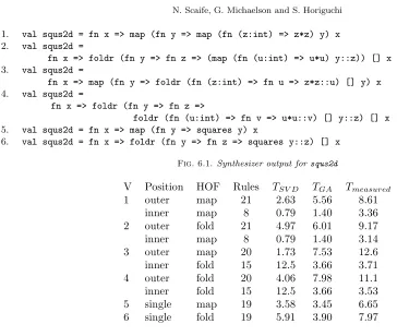
6. Performance Prediction Example. As part of the PMLS project we have used proof-planning to construct a synthesiser which extracts HOFs from arbitrary recursive functions [10]. For example, given the following program which squares the elements of a list of lists of integers:
fun squares [] = []
| squares ((h:int)::t) = h*h::squares t
fun squs2d [] = []
| squs2d (h::t) = squares h::squs2d t
the synthesizer generates the six programs shown in Figure 6.1. Note that there is no parallelism in this program suitable for our compiler and we would expect our predictions to validate this.
3
1. val squs2d = fn x => map (fn y => map (fn (z:int) => z*z) y) x
2. val squs2d =
fn x => foldr (fn y => fn z => (map (fn (u:int) => u*u) y::z)) [] x
3. val squs2d =
fn x => map (fn y => foldr (fn (z:int) => fn u => z*z::u) [] y) x
4. val squs2d =
fn x => foldr (fn y => fn z =>
foldr (fn (u:int) => fn v => u*u::v) [] y::z) [] x
5. val squs2d = fn x => map (fn y => squares y) x
6. val squs2d = fn x => foldr (fn y => fn z => squares y::z) [] x
Fig. 6.1. Synthesizer output forsqus2d
V Position HOF Rules TSV D TGA Tmeasured
1 outer map 21 2.63 5.56 8.61
inner map 8 0.79 1.40 3.36
2 outer fold 21 4.97 6.01 9.17
inner map 8 0.79 1.40 3.14
3 outer map 20 1.73 7.53 12.6
inner fold 15 12.5 3.66 3.71
4 outer fold 20 4.06 7.98 11.1
inner fold 15 12.5 3.66 3.53
5 single map 19 3.58 3.45 6.65
6 single fold 19 5.91 3.90 7.97
Fig. 6.2.Predicted and measured instance function times (µS)
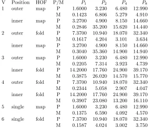
We require the execution times for the instance functions to the mapand foldrHOFs. We have not yet automated the collection of this data or linked the output from the performance prediction into the compiler so we present a hand analysis of this code.
Figure 6.2 shows the predicted instance function execution times for the two fitting methods alongside the actual measured times. The input data is a 5×5 list of lists of integers. The predictions are in roughly the correct range but differ significantly from the measured times. Despite the greater accuracy of the SVD fit to the learning-set data, the GA-generated weights give more consistent results compared to actual measured values. This is due to the numerical instability of the SVD fit. However, these discrepancies are sufficient to invert the execution times for nested functions. For instance, for Version 3 the inner fold instance function takes longer than the outer one, even though the outer computation encompasses the inner.
Applying the skeleton performance models to the measured instance function times, plus data on com-munications sizes gathered from sequential executions, gives the predicted parallel run-times for 1, 2, 4 and 8 processors, shown in Figure 6.3.
The GA- and SVD-predicted instance function times give identical predictions for parallel run-times. This is because the parallel performance model is in a range where the run-time is dominated by communications rather than computation. However, theP1 predictions are erroneous. These predictions represent an extrapolation of
a parallel run onto a sequential one which has no overheads such as communication. This also applies to the P2predictions, where these overheads are not accurately apportioned. Furthermore, the absolute values of the
predictions are unreliable. For the P8 values, some are accurate but some are out by an order of magnitude.
The most relevant data in this table is the ratio between the P4 and P8 values. This, in most cases, increases
as the number of processors increases, indicating slowdown.
7. Conclusions. Overall, our experimentation gives us confidence that combining automatic profiling with cost modeling is a promising approach to performance prediction. We now intend to use the system as it stands in implementing a performance-improving transformation system for a subset of the SML language. As well as exploring the automation of load balancing, this gives us a further practical way to assess the broader utility of our approach.
V Position HOF P/M P1 P2 P4 P8
1 outer map P 1.6000 3.230 6.480 12.990
M 0.1423 6.806 5.279 4.910
inner map P 3.2700 4.900 8.150 14.660
M 0.2846 35.200 15.620 14.440
2 outer fold P 7.3700 10.940 18.070 32.340
M 0.1617 4.204 3.101 3.634
inner map P 3.2700 4.900 8.150 14.660
M 0.3040 35.360 14.900 14.940
3 outer map P 1.6000 3.230 6.480 12.990
M 0.2205 7.314 3.923 4.739
inner fold P 14.2000 17.760 24.900 39.170
M 0.3875 26.020 14.570 15.770
4 outer fold P 7.3700 10.940 18.070 32.340
M 0.2344 5.058 2.907 4.047
inner fold P 14.2000 17.760 24.900 39.170
M 0.3907 23.080 13.200 16.110
5 single map P 1.6000 3.230 6.480 12.990
M 0.1375 6.590 4.092 4.570
6 single fold P 7.3700 10.940 18.070 32.340
M 0.1587 4.024 3.002 3.750
Fig. 6.3.Predicted (P) and measured (M) parallel run-times (mS)
and testing of the profiling mechanism but has wider implications for the development process where it could be useful for example to help the compiler when it is unable to get accurate predictions or gets stuck in the search space. Note that since our ultimate goal is fully automated parallelism we have not elaborated upon this point.
While we have demonstrated the feasibility of semantics-based profiling for an entire extant language, further research is needed to enable more accurate and consistent predictions of performance from profiles. Our work suggests a number of areas for further study:
• introducing non-linear costs into the system relating profile information and runtime measurements. The system would no longer be in matrix form and may require the use of generalised function min-imisation instead of deterministic fitting;
• identifying which semantic rules counts are most significant for predicting run times, through standard statistical techniques for correlation and factor analyses. Focusing on significant rules would reduce profiling overheads and might enable greater stability in the linear equation solutions;
• investigating the effects on prediction accuracy of optimisations employed in the back end compiler. Such optimisations fundamentally affect the nature of the association between the language semantics and implementation;
• systematically exploring the relationship between profiles and run-times for one or more constrained classes of recursive constructs, in the presence of both regular and irregular computation patterns. Our studies to date have been of very simple functions and of unrelated substantial exemplars;
• modeling explicitly aspects of implementation which are subsumed in the semantics notation. In partic-ular the creation and manipulation of name/value associations are hidden behind the semantic notion ofenvironment.
Acknowledgement. This work was supported by the Japan JSPS Postdoctoral Fellowship P00778 and UK EPSRC grants GR/J07884 and GR/L42889.
REFERENCES
[2] M. Aldinucci, S. Gorlatch, C. Lengauer, and S. Pelegatti,Towards Parallel Programming by Transformation: The FAN Skeleton Framework, Parallel Algorithms and Applications, 16 (2001), pp. 87–122.
[3] M. Alt, H. Bischof, and S. Gorlatch,Program Development for Computational Grids Using Skeletons and Performance Prediction, Parallel Processing Letters, 12 (2002), pp. 157–174.
[4] A. W. Appel, B. F. Duba, and D. B. MacQueen,Profiling in the Presence of Optimization and Garbage Collection, Tech. Report CS-TR-197-88, Princeton University, Dept. Comp. Sci., Princeton, NJ, USA, November 1987.
[5] H. Bischof, S. Gorlatch, and E. Kitzelmann,Cost optimality and predictability of parallel programming with skeletons, in Europar 03, vol. 2790 of LNCS, Jan 2003, pp. 682 – 693.
[6] T. Bratvold, Skeleton-based Parallelisation of Functional Programmes, PhD thesis, Dept. of Computing and Electrical Engineering, Heriot-Watt University, 1994.
[7] D. Busvine,Implementing Recursive Functions as Processor Farms, Parallel Computing, 19 (1993), pp. 1141–1153. [8] C. Cohen,Computer-Assisted Microanalysis of Programs, Communications of the ACM, 25 (1982), pp. 724–733. [9] M. I. Cole,Algorithmic Skeletons: Structured Management of Parallel Computation, Pitman/MIT, 1989.
[10] A. Cook, A. Ireland, G. Michaelson, and N. Scaife,Discovering Applications of Higher-Order Functions through Proof Planning, Formal Aspects of Computing, 17 (2005), pp. 38–57.
[11] K. Hammond, J. Berthold, and R. Loogen,Automatic Skeletons in Template Haskell, Parallel Processing Letters, 13 (2003), pp. 413–424.
[12] D. L. M´etayer,ACE: An Automatic Complexity Evaluator, ACM TOPLAS, 10 (1988), pp. 248–266.
[13] G. Michaelson and N.Scaife,Parallel functional island model genetic algorithms through nested skeletons, in Proceedings of 12th International Workshop on the Implementation of Functional Languages, M. Mohnen and P. Koopman, eds., Aachen, September 2000, pp. 307–313.
[14] G. Michaelson and N. Scaife,Skeleton Realisations from Functional Prototypes, in Patterns and Skeletons for Parallel and Distributed Computing, F. Rabhi and S. Gorlatch, eds., Springer, 2003.
[15] R. Milner, M. Tofte, and R. Harper,The Definition of Standard ML, MIT, 1990.
[16] G. D. Plotkin,A Structural Approach to Operational Semantics, Tech. Report DAIMI FN-19, Arrhus University, Denmark, Sep 1981.
[17] W. H. Press, S. A. Teukolsky, W. T. Vetterling, and B. P. Flannery,Numerical Recipes in C, CUP, 2nd ed., 1992. [18] R. Rangaswami,A Cost Analysis for a Higher-Order Parallel Programming Model, PhD thesis, University of Edinburgh,
1995.
[19] N. R. Scaife,A Dual Source, Parallel Architecture for Computer Vision, PhD thesis, Dept. of Computing and Electrical Engineering, Heriot-Watt University, 1996.
Edited by: Fr´ed´eric Loulergue
Received: November 14, 2005