Macroscopic Visualization of the Heart Electrical Activity Via
an Algebraic Computer Model
A. Ghaffari*, M. R. Homaeinezhad**, Y. Ahmadi**, M. Rahnavard** and R. Rahmani***
Abstract: In this study, a mathematical model is developed based on algebraic equations which is capable of generating artificially normal events of electrocardiogram (ECG) signals such as P-wave, QRS complex, and T-wave. This model can also be implemented for the simulation of abnormal phenomena of electrocardiographic signals such as ST-segment episodes (i.e. depression, elevation, and sloped ascending or descending) and repolarization abnormalities such as T-Wave Alternans (TWA). Event parameters such as amplitude, duration, and incidence time in the conventional ECG leads can be a good reflective of heart electrical activity in specific directions. The presented model can also be used for the simulation of ECG signals on torso plane or limb leads. To meet this end, the amplitude of events in each of the 15-lead ECG waveforms of 80 normal subjects at MIT-BIH Database (www.physionet.org) are derived and recorded. Various statistical analyses such as amplitude mean value, variance and confidence intervals calculations, Anderson-Darling normality test, and Bayesian estimation of events amplitude are then conducted. Heart Rate Variability (HRV) model has also been incorporated to this model with HF/LF and VLF/LF waves power ratios. Eventually, in order to demonstrate the suitable flexibility of the presented model in simulation of ECG signals, fascicular ventricular tachycardia (left septal ventricular tachycardia), rate dependent conduction block (Aberration), and acute Q-wave infarctions of inferior and anterior-lateral walls are finally simulated. The open-source simulation code of above abnormalities will be freely available.
Keywords: Electrocardiogram(ECG), Mathematical Model, Heart Arrhythmia, Simulation.
1 Introduction
First models of heart refer to middle age and renaissance era depicted in the Leonardo da Vinci’s drawings [1]. Generally, modeling is an abstraction by which it would be possible to move from the known to the unknown as to the resulted model is consistent with observations and can be used for the prediction of unobserved set. The major aims of modeling can be summarily stated as management and control, prediction and simulation of phenomena, as well as education and familiarity with complicated understudy phenomena [1,
Iranian Journal of Electrical & Electronic Engineering, 2009. Paper first received 15 Jan. 2009 and in revised form 7 May 2009. * Professor of Mechanical Engineering, Department of Mechanical Engineering, K. Nassir Toosi University of Technology.
E-mail: [email protected]
** Members of Cardio Vascular Research Group (CVRG), Department of Mechanical Engineering, K. Nassir Toosi University of Technology.
E-mail: [email protected].
*** Assistant Professor of Cardiology, Tehran University of Medical Science, Member of Cardiovascular and Catheter Unit of Imam
2]. Modeling of the electrical activity of heart as a
complicated system can be conducted using
microscopic methods which are based on cellular structure and dynamics, cellular automata [3], and reaction diffusion systems [4], or macroscopic approaches which are based on observed electrical behavior of the heart on the skin surface [5, 6]. Single-lead [5], multi-Single-lead [7] and high-resolution multi-Single-lead [8, 9] electrocardiographic signals as electrical skin surface recordings can be a useful way in the macroscopic modeling of the heart. Some events in the electrocardiogram signals are indicators of specific electrocardiographic occurrences, the most typical of which in normal conditions are P-wave, QRS complex, and T-wave (Sometimes U-wave) that happen relative to each other with regular duration. Furthermore, the morphology of P, QRS, and T waves can vary in different leads regarding the fact that each lead illustrates a distinct picture of the heart electrical activity in a specific direction [10, 11]. For instance, when the ventricular septum is normally depolarized from the left side to the right side, R-wave and Q-wave will be observed in chest leads V1 and V6, respectively.
However, in the depolarization of the ventricular main muscle mass, S-wave and R-wave will instead be seen in leads V1 and V6 [10]. Depending upon the distance and orientation of the lead relative to the heart, the amplitudes of waves in each lead will differ from those in the other leads [10, 12].
The aim of this study is to achieve knowledge about the distribution of wave amplitudes relative to each other in a single ECG lead and relative to their corresponding waves in the other leads as well as developing a model based on this information in order to simulate some normal and abnormal events. To meet this end, the amplitude of events in each of the 15-lead ECG waveforms of 80 normal subjects at MIT-BIH Database (www.physionet.org) are derived and recorded. Various statistical analyses such as amplitude mean value, variance and the corresponding confidence intervals calculations, Anderson-Darling normality test [13], and Bayesian estimation of events amplitude are then conducted. A Gaussian (normal) probability density function (pdf) is then assumed for each of event differences with mean values and variances obtained from statistical analyses. Afterwards, a Bayesian estimator of the elevation of each event in all leads is designed with the amplitude of P-wave in lead 1 as an input. If so, the 15-lead ECG signal generator will consequently be created. In order to simulate the
interaction of regulating sympathetic and
parasympathetic mechanisms in the modulation of QRS complexes, the original work of McSharry-Clifford (2003) [5] is used in the next step and waves with HF/LF and VLF/LF power ratios (HF: high frequency, LF: low frequency and VLF: very low frequency), are incorporated to the power spectrum of RR-tachogram [5, 14]. The resulted algebraic model of this study has the following characteristics:
• The model parameters have independent effects on the model output events, i.e. the amplitude, duration, and incidence time of each event can directly be considered as inputs to the program.
• This model is capable of generating transient ST-segment episodes such as depression, elevation, and sloped ascending or descending, [15].
• This model consists of algebraic mathematical equations Therefore, there would be no need to numerical solution routines.
Finally, to illustrate the capabilities and flexibility of the presented model in generating artificial arrhythmias and ECG signal abnormalities, fascicular ventricular tachycardia (left septal ventricular tachycardia), rate dependent conduction block (Aberration), and acute Q-wave infarctions of inferior and anterior-lateral walls
are simulated. The open source simulation code of the aforementioned abnormalities will be freely available.
2 Statistical Analysis of Wave Amplitudes
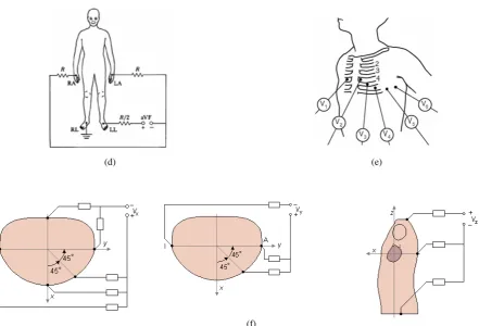
For the aim of statistical analyses of events amplitudes and finding the corresponding relation between them in each lead, the 15-lead ECG data of 80 normal subjects were derived from the MIT-BIH DATABASE (www.physionet.org). The position of electrodes on the body surface related to each lead can be seen in Fig. 1. The wave amplitudes of each lead were then obtained and recorded by implementing the wave detection algorithm of WaveForm DataBase (WFDB), [16]. The difference between the events amplitudes, i.e. P-Q, P-R, P-S, P-T, Q-R, Q-S, Q-T, R-S, R-T, and S-T were then calculated for all 15-lead ECGs. It should be noted that Q-waves were not observed in some leads such as MLV1, MLV2, and MLV3 (see Table 2). Statistical analyses such as mean value and variance, and the corresponding confidence intervals calculations were then conducted as follows.
Confidence interval (CI) of a parameter which has wide applications in engineering statistical analyses is actually an interval estimate of that parameter and has two characteristics: First, the point estimation of the parameter is located in this interval. Second, there would be a high probability for the true value of the parameter to belong to this interval. In this study, the results of the CI and variance calculations will be presented. More information about the CI and variance equations and the corresponding calculations can be found at [13].
To calculate the CI, it can be shown that if µˆSM and
2 ˆSV
σ represent the mean value and variance of n number of samples from a random population (X=x1,x2,...,xn)
with normal distribution and unknown variance, then a confidence interval of 100(1-α) % for the true mean
value of observations, µT , can be obtained from the
following equations, [13], ˆ
( 2 , 1)
ˆ
ˆ
( 2, 1)
ˆ
SV
SM T
SV
T SM
t n
n
t n
n
α
σ
µ
µ
α
σ
µ
µ
−
− ≤
−
≤ +
(1)
where
(
)
− −
= =
∑
∑
= =
n
k
SM i SV
n
k i SM
x n
x n
1
2 2
1
ˆ 1
1 ˆ
1 ˆ
µ σ
µ
(
2)in which, t(
τ
,n) is 100×τ percentage point fromt-distribution of n degrees of freedom and can be obtained from the following equation
∫
+∞= )
,
( n (, )
tα pT t n dt
α
(3)and,
[
( 1) 2]
1( , )
( 1) / 2 2
( 2) ( / ) 1
n t n
T k
n n
t n
t
p
π Γ +
= +
Γ +
− ∞ < < +∞
(4)Also to find the CI for the variance, If µˆSM and
2 ˆSV
σ
represent the mean value and variance of n number of samples from a random population with normal distribution (X=x1,x2,...,xn) and with unknown
variance, then a confidence interval of 100(1-α) % for
the true variance of observations, 2
T
σ , can be obtained from the following equation
) 1 , 2 / 1 (
ˆ ) 1 ( ˆ
) 1 , 2 / (
ˆ ) 1 (
2
2 2
2
2
− −
− ≤
≤ − −
n n
n
n SV
T SV
α
χ
σ
σ
α
χ
σ
(5)
where 2( /2, −1) n α
χ and 2(1− /2, −1)
n α
χ are the
upper and lower 100×α/2 percentile points of the
chi-square distribution of degrees of freedom n-1,
respectively, and can be calculated as, [13]
∫
+∞= )
, (
2αn p 2(x,n)dx
χ χ α (6)
0 , )
2 ( 2
1 )
,
( (/2)1 /2
2 /
2 >
Γ
= − −
x e x n n
x
p n x
n
χ (7)
2.1 Anderson- Darling Distance Test
In many applications, in order to provide the required prerequisites for the design of estimation and identification algorithms, we need to determine a distribution function which most probably describes the distribution of conducted observations. On the other hand, if the probability density function is considered for the observations set Ω, the structure of the corresponding estimator will implicitly be determined. In this study, a method called Anderson-Darling Distance Test (ADDT) is used for the calculation of goodness of fit relative to normal distribution. In this method, a statistic is defined on the basis of the following integral transform
∫
−∞= x p s ds x
F( ) ( ) (8)
Using the mapping in the above integral, a certain distribution with the density p(x) is converted to a uniform distribution. If so, it can be concluded that for independent and identically distributed (i.i.d.) random variables x1, x2,…, xn with cumulative distribution function (CDF) of F(x), the functions F(x1), F(x2),…, F(xn) will be independent uniform random variables in the interval (0,1). In fact, Anderson-Darling Distance Test indicates how much closer is the value of F(x1), F(x2),…, F(xn) to the uniform distribution in the interval (0,1) [13].
In the ADDT it is assumed that the observation domain data are the members of a discrete random variable. For each x∈Ω, the value of F(X≤x)is then calculated and restored. The best straight line crossing the points (x, F(x)) was next determined. The mean absolute distance value of the points relative to this line can be obtained as
∑
= −= in i i
R
MAD F x L x
n AD
1 )
(
) ( ) ( 1
(9)
where L(x) represents the equation of the line in the (x, F(x)) plane. Using the Monte-Carlo algorithms [17], a sequence of the numbers belonging to a normal random population with known mean value and variance of the observation set was generated. The parameter (N)
MAD
AD for this sequence will then be calculated from the lineL(x). Afterwards, the fraction N
MAD R
MAD AD
AD is
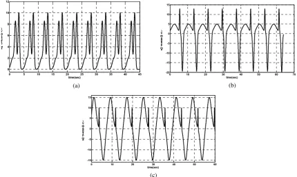
determined and compared with a specific threshold. If the fraction is greater than τ, the normality assumption will be rejected. In this study, the value τ=2.2 is selected and the results of the normality test for the differences T-P, R-Q, and R-P are presented in Tables 1 to 3. In Figs. 2 and 3, the probability F(X≤x) versus observation domains is plotted for the leads II and Vx. According to ADDT, when the values of probability
)
( x
F X≤ are remarkably far from the straight line L(x) or build a curvature, the normality assumption for the data distribution cannot be acceptable. This can be observed in the Figs. 2 and 3.
(a) (b) (c)
(d) (e)
(f)
Fig. 1. Overview of the landmarks used for the generation of heart electrical pictures; (a) Limb Leads I, II and III, (b) Lead avL, (c)
Lead avR, (d) Lead avR [18], (e) Chest Leads [10], (f) Frank Vx, Vy and Vz leads [19]
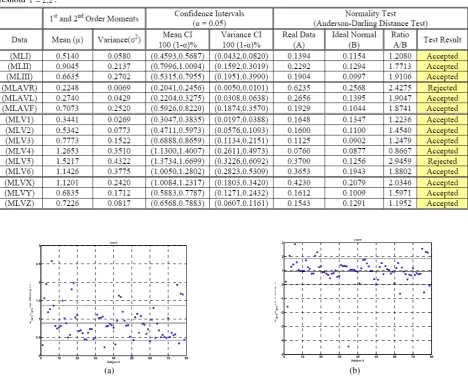
Table 1. Results of the statistical analyses conducted on the T-wave and P-wave amplitudes differences for the 15-lead ECGs: Mean
value, variances, the corresponding confidence intervals with the value of α=0.05 and Anderson-Darling Normality Test using a
threshold τ=2.2.
Table 2. Results of the statistical analyses conducted on the R-wave and Q-wave amplitudes differences for the 15-lead ECGs: Mean
value, variances, the corresponding confidence intervals with the value of α=0.05 and Anderson-Darling Normality Test using a
threshold τ=2.2.
Table 3. Results of the statistical analyses conducted on the R-wave and P-wave amplitudes differences for the 15-lead ECGs: Mean
value, variances, the corresponding confidence intervals with the value of α=0.05 and Anderson-Darling Normality Test using a
threshold τ=2.2.
0 10 20 30 40 50 60 70 80
0 0.5 1 1.5 2 2.5 3
Subject # Ra
mp
-P
a mp
A m plit u d e< m V >
Lead II
0 10 20 30 40 50 60 70 80
-5 -4 -3 -2 -1 0 1 2 3
Subject # Ra
mp
-Qa
mp
A mpl it u d e< m V>
Lead II
(a) (b)
0 10 20 30 40 50 60 70 80 -0.1
0 0.1 0.2 0.3 0.4 0.5 0.6 0.7
Subject # Ta
mp
-P
a mp
A mpl it u d e< mV >
Lead II
0 0.5 1 1.5 2 2.5
0.01 0.02 0.05 0.10 0.25 0.50 0.75 0.90 0.95 0.98 0.99
Observation Domain Pr
o b a bil it y
R-P Chart MLII
(c) (d) (Accepted) (AD = 1.7713)
-4 -3 -2 -1 0 1 2 3
0.01 0.02 0.05 0.10 0.25 0.50 0.75 0.90 0.95 0.98 0.99
Observation Domain P
r o b a b il it y
R-Q Chart MLII
-0.1 0 0.1 0.2 0.3 0.4 0.5 0.6 0.01
0.02 0.05 0.10 0.25 0.50 0.75 0.90 0.95 0.98 0.99
Observation Domain Pr
o ba bil it y
T-P Chart MLII
(e) (Accepted) (AD = 1.8534) (f) (Accepted) (AD = 1.0155)
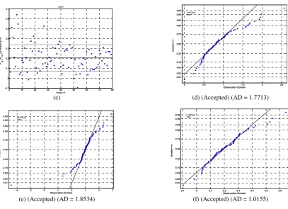
Fig. 2. (a,b,c): Dispersion of the data obtained from the wave amplitude difference calculations in lead II. The solid and dashed lines
represent the mean value, µ−σ and µ+σof the data, respectively.
(d,e,f): The probability F(X≤x) versus observation domain plot. The straight solid line represents the best line which can be fitted to
the probabilities. The triangles illustrate the calculated probabilities. The normality test will be rejected in the cases that the triangles are far from the straight line or show high curvature.
0 10 20 30 40 50 60 70 80
0 0.5 1 1.5 2 2.5 3 3.5 4
Subject # Ra
mp
-Pa
mp
A mpl it u d e< mV >
Lead vx
0 10 20 30 40 50 60 70 80
0 0.5 1 1.5 2 2.5 3 3.5 4 4.5
Subject # Ra
mp
-Qma
p
A m plit u d e< mV >
Lead vx
(a) (b)
0 10 20 30 40 50 60 70 80
-0.2 0 0.2 0.4 0.6 0.8 1 1.2
Subject # Ta
mp
-P
a mp
A m plit ud e< m V >
Lead vx
0 0.5 1 1.5 2 2.5 3 3.5
0.01 0.02 0.05 0.10 0.25 0.50 0.75 0.90 0.95 0.98 0.99
Observation Domain Pr
o b a b il it y
R-P Chart MLVx
(c) (d) (Accepted) (AD = 2.0346)
0 0.5 1 1.5 2 2.5 3 3.5 4 0.01
0.02 0.05 0.10 0.25 0.50 0.75 0.90 0.95 0.98 0.99
Observation Domain Pro
b a b il it y
R-Q Chart MLVx
0 0.2 0.4 0.6 0.8 1
0.01 0.02 0.05 0.10 0.25 0.50 0.75 0.90 0.95 0.98 0.99
Observation Domain P
r o b a bil it y
T-P Chart MLVx
(e) (Accepted) (AD = 1.9321) (f) (Accepted) (AD = 1.0167)
Fig. 3. (a,b,c): Dispersion of the data obtained from the wave amplitude difference calculations in lead Vx. The solid and dashed lines
represent the mean value, µ−σ and µ+σof the data, respectively.
(d,e,f): The probability F(X≤x) versus observation domain plot. The straight solid line represents the best line which can be fitted to
the probabilities. The triangles illustrate the calculated probabilities. The normality test will be rejected in the cases that the triangles are far from the straight line or show high curvature.
2.2 Discussion
Regarding the performed statistical analyses, it can be seen that for differences T-P, R-Q and R-P, according to the ADDT, there are approximately 14.3% cases among all leads that fail the normality test. It is obvious that the normality test rejection (NTR) percent has inverse proportion to the threshold
τ . Loosely speaking, if threshold τ is chosen a large number say 4, most of the A/B ratios will remain under the threshold. Thus, NTR will tend to zero and consequently test does not reject the normality hypothesis. For ADDT, if threshold τ is chosen to be
5 . 2 2 .
1 ≤τ≤ , acceptable results would be expected from the test, [13]. In this study, by selecting τ=2.2, it is shown that approximately 85.7% of all aforementioned differences, suitably pass the ADDT. This result can satisfactorily be generalized and applied to the remained differences omitted to appear in this study. It should be noted that according to the Central Limit Theorem (CLT), [13], if the number of samples chosen from random population is large enough, behavior of the selected population can be expected to be normal. Accordingly, due to sufficient number of subjects studied in this paper, the behavior of most of the differences will approximately be close to the normal distribution. Implementing the fact that the ADDT illustrates normal behavior of differences in most of the leads, the structure of appropriate estimators can be designed on the basis of various strategies. As a case in view, in this study it is assumed that the amplitude of the P-wave in lead I is measured and the amplitudes of the remaining waves in the same lead and the other leads are estimated by applying the proper estimator. Therefore, with the aid of this method a useful tool can be designed using which different electrical pictures of the heart electrical activity can be obtained. So far, numerous algorithms have been designed and developed based upon the finite element
methods, [20], to generate such electrical pictures. Although acceptable results can be gained using these algorithms in normal cases and some arrhythmias; however, they have their own specific limitations. The major advantage of the presented model of our study is that it almost has no limitation in the generation of the artificial ECG signals. It will be demonstrated that how complicated arrhythmias can be generated using this model.
3 Description of the Algebraic Model of Artificial ECG Generator
The presented mathematical model is based on the idea that the overall generated artificial signal is developed by the superposition of some events with least similarities in their domains. Indeed, the amplitude of event k has no effect on the amplitude of the events k−1 and k+1, unless these two events are significantly close to each other. The studies conducted in this field indicate the fact that electrocardiogram waves generated due to the heart depolarization (i.e. P-wave and QRS complex) will have rather symmetric morphologies; however, the repolarization waves such as T-wave will be asymmetric on the skin surface due to the impulsive and asymmetric morphology of the action potential on the epicardial surface [1, 20, 21]. Accordingly, assume that the event
i
in the electrocardiogram signal of the lead j and heart beatk is defined as
(
)
− −
= 2
2 ( ) ( )
) ( 2
1 exp ) ( ) ,
( s k k
k k
C s k
E j ij
ij ij
ij µ
σ (10)
whereCij, σij, µij are the corresponding parameters of
the event Eij and should be determined as to the event
could be generated using the arbitrary amplitude, incidence time, and duration. According to the Eq. 10, it is obvious that the function Eij(s) has a single extremum value of Cij at s=µij .Thus, Cij and µij
will represent the incidence amplitude and incidence time along the s-axis, respectively. In order to evaluate the duration of eventEij(s), the event start point is illustrated by ij
ON
s and the end point is depicted with ij
OFF
s . It is supposed that function Eij(s) has an infinitesimal positive value of
ε
in the position ijON
s or ij
OFF
s . Therefore,
(
)
(
)
= − − ⇒ − − = ) ( ln ) ( ) ( ) ( 2 1 ) ( ) ( ) ( 2 1 exp ) ( 2 2 2 2 k C k k s k k k s k k C ij ij OFF ij ij ij OFF ij ij ij ε µ σ µ σ ε (11)If half of the duration of the event Eij(s) is equal to )
( ) ( )
(k s k ij k
ij OFF
ij µ
ξ = − , then
) ( ) ( ln ) ( 1 ) ( 2 1 ) ( ) ( 2 2 2 k k C k k k k s ij ij ij ij ij ij OFF ij λ ε ξ σ ξ µ − = = − ⇒ = − (12)
and the Eq. 10 can be re-written as:
(
)
[
2( ) ( ) ( ) 2]
exp ) ( ) , ( k k s k k C s k E ij j ij ij ij µ λ − − × = (13)
Consequently, with the values of the
parametersCij,λij,µij known, the amplitude, duration
and incidence time for the event Eij(s) will be determined independently. The superposition of these events can be a good approach to the development of an exhaustive set of all waveforms in the lead j, as follows
{
}
(
)
[
]
U
U U
B j B j N k N i ij j ij ij N k N i ij j k k s k k C s k E s E 1 1 2 2 1 1 ) ( ) ( ) ( exp ) ( ) , ( ) ( = = = = − − = =∑
λ µ(14)
where Cij(k) and µij(k) represent the incidence amplitude and incidence time of the k-th beat along the s-axis, respectively. Note that the index ij indicates event i in the lead j. λij(k) is i-th event in j-th lead duration parameter that if is chosen according to Eq. (12), desired duration will be obtained. In Eq. (14), it is assumed that the independent variable sj(k) is an arc length of a circle with an origin in θ=0, and when
t ω
θ= , it will be equal to s=rωt (see Fig. 4). It should also be mentioned that all events in a heartbeat will occur in a complete revolution on the circle. Therefore, with a heart period of τ for a complete heartbeat, the circular frequency for the revolution on a circle with radius r will equal
τ π
ω=2 . Given the values of the parameters Cij(k), tijµ(k)
and tijξ(k) by the user, the parameter values of λij(k) and µij(k)in Eq. 10 for the event i in the lead j can be obtained from the following equation
= − ⇒ = = ) ( ln ) ( 1 ) ( ) ( ) ( ), ( ) ( 2 2 k C k k k t r k k t r k ij ij ij ij ij ij ij
ε
ξ
λ
ω
ξ
ω
µ
ξ µ (15)3.1 Adding Transient ST Segment Episodes to the Algebraic Model
With the aim of modeling the effects of transient ST-episodes (TSE), an event with three distinct parts is considered in this section. The beginning and last parts are each consisting of the half of the Eq. 10 function, and a straight line with a positive, negative, or zero slope will connect these two parts. Therefore, a TSE wave will be characterized by 6 parameters, namely as
) (k
ij
ξ′ , ξij′′(k), Cij′(k), m′ij(k), µij′(k), µij′′(k), which are schematically illustrated in Fig. 5. The ascending and descending rate of the ST-segment can be adjusted using the parameter mij′(k). With the values of the parameters µij′(k) and µij′′(k) equal to each other, an asymmetric T-wave, which is close to reality [12], will be generated.
3.2 Adding Heart Rate Variability (HRV) to the Algebraic Model
The artificial RR-tachogram algorithm developed by McSharry-Clifford, 2003 [5], is implemented in this study in order to include the effect of HRV in the presented algebraic model. In their model, RR-tachogram could be generated with the adjustment of
the power spectrum of RR time series using fast Fourier Transform (FFT) and inverse Fourier Transform [5, 14]. In this study, the power spectrum of RR time series in rest position is approximated with VLF/LF and HF/LF power ratios and the resulted RR
sequence is added to the algebraic model. In order to adjust the RR distances in the algebraic model, suppose that RRj(k) represents the distance between two subsequent R-peaks in the heartbeats k-1 and k. Also assume that the time period of the complete heartbeat k in the lead j is equal to τj(k).
If so, the position of all R-peaks can be obtained from the following recursive equation. For the value
R
i= , tijµ(k)
represents the position of peak R in the beat k
=
− +
=
R i
k RR k t k
tijµ( ) ijµ( ) j( 1)
(16)
If the end point of the beat k in the lead j is illustrated by EPj(k), then τj(k)can be calculated from the following equation
=
× = −
R i
k t
k EP k
tijµ( ) j( ) ijµ(1) τj( )
(17)
=
− =
R i
t k EP k t k
ij j ij
j
) 1 (
) ( ) ( )
( µ
µ
τ
(18)
Finally, the following recursive equation can be used for the calculation of the end point of the beat k
) ( ) 1 ( )
(k EP k k
EPj = j − +τj (19)
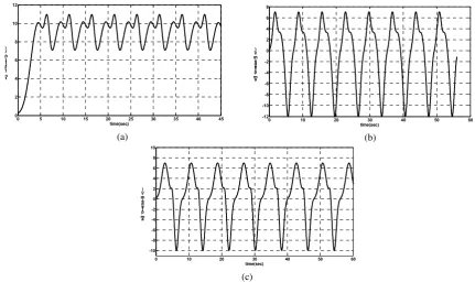
Solving the Eqs. 15 to 19, the end point of each heartbeat can be obtained as a function of instantaneous artificial heart rate, as to the time sequence RRj(k) will be similar to the artificial values. Modulation of the QRS complexes using the presented algorithm is illustrated in Fig. 6. The effect of respiration is added to the model using a sinusoid signal with certain amplitude and frequency. A normal additive noise with the mean value of zero and
variance 2 6
10−
=
σ is also added to the model as the measurements noise in order to increase the similarity of the model to the actual signals.
Fig. 4. The definition of the variable s=rωt and its positive direction. It is assumed that an object with the
angular velocity ω moves on a circle with the radius r
Fig. 5. Representation of the transient ST-segment Episodes
(TSE). Each TSE is specified by 6 parametersξij′(k),
) (k
ij
ξ′′ , Cij′(k), m′ij(k), µij′(k), µij′′(k), and can have a
positive, negative, or zero slope.
2 4 6 8 10 12 14 16 18 20
0 0.05 0.1 0.15 0.2 0.25
time(sec) a
m plit u d e( m V)
4 .5 5 5. 5 6 6. 5 7
0
0 . 0 5
0 . 1
0 . 1 5
0 . 2
Fig. 6. Modulation of QRS complexes based on Eq.s 17 to 19 using artificial RR-tachogram generator introduced in [9]
3.3 Design of Bayesian Estimator of WaveAmplitude Algebraic Model
In section B it was shown that the differences between the waves amplitudes can be cast in a probabilistic framework. Thus, it will determine the estimator structure after the selection of estimation strategy. In this study, we have used the idea that the
) (k
ij
µ′ µij′′(k)
) (k
ij
ξ′ ξij′′(k)
) (k
Cij′ Slope m(k)
ij
′ = y
r
t
ω θ=
+
t r s= ω
x
probability density function of the P-wave amplitude in the lead I is determined using statistical analyses and the amplitude of all other waves in the same lead and other leads can then be determined with the observation of the P-wave amplitude in the lead I.
It should be noted that there is a wide definition for the expression of normality (healthy) in the medical terminology (for instance a “normal” fat smoker and a “normal” young athlete). Therefore, the designed estimator will not be capable to present precise results. The reasonable, but not accurate, predictions of the presented model using the collected data is the most significant point of the presented strategy.
Assume the random variable X defined in the
domain Ω, i.e.
{
Ω}
X x∈
p ; wherepX is the
probability density function forX=x, specifies a family of distributions for the random observationY. Also, suppose that the random observation Y has the values y defined in the domain Γ. It is aimed to determine a mapping like xˆ:Γ→Ω as to xˆ(y)be the best guess for random variable X for the observed value Y=y. To meet this end, a cost function of
R
Ω
Ω× →
:
C is defined, in which C[xˆ(y),x] is the imposed cost of the estimation of the actual value of the random variable X with the valuexˆ(y). If so, cost average over Y for each x∈Ω can be defined as follows, [17],
[
]
{
Cx x x}
E x
Rx(ˆ)= ˆ(Y), X= (20)
Regarding this equation, the Bayesian Risk which is in fact the mean value of the cost average Rx(xˆ) can be described as
{
}
[
]
{
}
[
]
{
}
{
Y X Y}
X Y X ), ( ˆ ), ( ˆ ) ˆ ( ) ˆ ( ) ˆ ( x C E E x C E x r x R E x r B B = = ⇒ = (21)
Accordingly, the Bayesian estimation of the random variable X for each value y∈Γ can easily be found by the minimization, if it exists, of the following posterior cost
[
]
{
C x y y}
E ˆ( ),X Y= (22)
If the random variable X has the probability density pX y(x y) for each Y= y, y∈Γ, then the Bayesian estimation xˆ(y)for each valuey∈Γ can be determined from the following equation
[
x y x]
p x y dxC
Ipr ˆ( ), Xy( )
Ω
∫
= (23)
In order to achieve the Minimum Mean Square Error (MMSE) estimation, the cost function C[xˆ(y),x] is defined as follows
[
]
(
)
2) ( ˆ ), (
ˆ y x x y x
x
C = − (24)
Since this cost function measures the estimator performance in terms of error square, it can be implemented in many cases and the resulted estimation will also have a closed form [17]. If so, the Bayesian estimator will be an MMSE estimator and the posterior cost for Y=y will be equal to
[
]
{
}
{
[
]
}
{
}
{
}
[
]
{
}
{
y}
E y E y x y x y E y y x E y y x E y y x E = + = − = = + = − = = = − Y X Y X Y X Y X Y Y X 2 2 2 2 2 ) ( ˆ 2 ) ( ˆ ) ( ˆ 2 ) ( ˆ ) ( ˆ (25)
As can be observed, the above equation is a quadratic function of xˆ(y) and can be re-written as follows
[
]
{
}
{
}
{
}
{
}
[
E y]
E{
y}
y E y x y y x E = + = − = − = = − Y X Y X Y X Y X 2 2 2 2 ) ( ˆ ) ( ˆ (26)
This expression will have its minimum value if the complete square expression controlled by xˆ(y)is equal to zero. Indeed
[
]
{
}
{
y}
E y x y y x E y x = = ⇒ = = − ∂ ∂ Y X Y X ) ( ˆ 0 ) ( ˆ ) ( ˆ 2 (27)
Solution of this equation will lead to a point in which the cost function achieves its unique minimum and the derivative of the cost function with respect to
) ( ˆ y
x is equal to zero.
The MMSE estimation will consequently be the average conditional value of the random variable X for Y=y. Thus, the random variable X should be averaged as follows
{
y}
E y
xˆ( )= X Y= (28)
If so, it is necessary to obtain a posterior conditional density (pXy(xy)) of the likelihood
function (pYx(yx)) using the following theorem:
Lemma 3: If pYx(yx) represents the conditional density (likelihood function), and random variables X
and Y have marginal density functions pX(x) and )
(y
pY respectively, then a posteriori density function,
) (xy
pXy can be obtained from the following equation,
[22]
∫
= =
Ω Y X
Y Y X Y X dx x p x y p y p y p x p x y p y x p x x y ) ( ) ( ) ( ) ( ) ( ) ( ) ( (29) Proof:
If F(⋅) represents the Cumulative Distribution Function (CDF), then
) ( lim ) ( 2 1 0 1 2 ∆ + ≤ < ∆ + ≤ < = = ∆ + ≤ < →
∆ F x x y y
y x x F Y X Y X (30)
Using the conditional probability function [23] properties, the latter equation can be written as
{
} {
}
(
)
(
2)
2 1 2 1 ) ( ∆ + ≤ < ∆ + ≤ < ∩ ∆ + ≤ < = ∆ + ≤ < ∆ + ≤ < y y F y y x x F y y x x F Y Y X Y X (31)
and the right side of the Eq. 31 will be as follows
{
} {
}
(
)
(
1)
1 2
2 1
)
( < ≤ +∆ < ≤ +∆ < ≤ +∆
= ∆ + ≤ < ∩ ∆ + ≤ < x x F x x y y F y y x x F X X Y Y X
(
)
(
2)
1 1 2 0 2 1 ) ( lim ) ( ∆ + ≤ < ∆ + ≤ < ∆ + ≤ < ∆ + ≤ < = = ∆ + ≤ < →
∆ F y y
x x F x x y y F y x x F Y X X Y Y X (32)
If the numerator and denominator of the right hand side of the Eq. 31 is divided by ∆2, then
(
)
(
)
2 2 1 2 1 2 0 2 1 ) ( lim ) ( ∆ ∆ + ≤ < ∆ + ≤ < ∆ ∆ + ≤ < ∆ + ≤ < = = ∆ + ≤ < →∆ F y y
x x F x x y y F y x x F Y X X Y Y X (33)
Also, if both sides of the Eq. 33 are divided by ∆1 and both ∆1 and ∆2 are tended to zero, i.e.
0 ,
0 2
1→ ∆ →
∆ , then
(
)
(
)
∆ ∆ + ≤ < ∆ ∆ + ≤ < ∆ ∆ + ≤ < ∆ + ≤ < = ∆ = ∆ + ≤ < → ∆ → ∆ → ∆ 1 1 2 2 2 1 2 0 2 0 1 1 1 0 1 ) ( lim lim ) (lim F x x
y y F x x y y F y x x F X Y X Y Y X (34)
According to the definition of the conditional density function in terms of conditional probability function [23] we have
) ( ) ( ) ( ) ( y p x p x y p y x
p y x
Y X Y
X = (35)
On the other hand, if the conditional density )
(yx
pYx and the marginal density pX(x) are both at hand, the marginal density pY(y) will simply be calculated by integrating Eq. 32 as follows
) ( ) ( ) ( ) ( y p x p x y p y x
p y x
Y X Y
X = (36)
Because according to the Eq. 32, we can write
) ( ) ( ) ,
(x y p yx p x
pXY = Yx X (37)
and this is the end of the proof. Therefore, using the Eqs. 28 and 36, xˆMMSE(y) can be derived from the following equation
{
}
ˆ
(
)
(
)
( )
(
)
( )
MM SE y x xx
E
y
x p
x y dx
x p
y x p
x dx
p
y x p
x dx
=
=
=
=
∫
∫
∫
X Ω X Y Ω X Y ΩX Y
(38)Assume X and Y to be two random variables, where X is a normal random variable with the density
) ,
( 2
x x
N µ σ and the random variable Y−X has the
normal pdf ( , 2) 0 0 σ µ
N . The likelihood density function
will then have the normal density pdf ( , 2) 0
0 σ
µ x
N +
for X=x and we have
) , ( ~ ) ( 2 0 0σ µ N X
Y− (39)
) , ( ~ 2 x x
N µ σ
X (40) − − − = + = 2 0 2 0 0 2 0 0 ) ( 2 1 exp 2 1 ) , ( ~ x y x N x µ σ σ π σ µ X Y (41)
According to the Eq. 38, the xˆMMSE(y)estimation using the observation y will be as follows
∫
∫
− − − − − − − − − − = Ω Ω dx x x y dx x x y x y x x x x x x x MMSE 2 2 2 0 2 0 0 2 2 2 0 2 0 0 ) ( 2 1 exp 2 1 ) ( 2 1 exp 2 1 ) ( 2 1 exp 2 1 ) ( 2 1 exp 2 1 ) ( ˆ µ σ σ π µ σ σ π µ σ σ π µ σ σ π (42)which can be simplified to the following equation
∫
∫
∞ + ∞ − ∞ + ∞ − − − − − − − − − − − = dx x x y dx x x y x y x x x x x MMSE 2 2 2 0 2 0 2 2 2 0 2 0 ) ( 2 1 ) ( 2 1 exp ) ( 2 1 ) ( 2 1 exp ) ( ˆ µ σ µ σ µ σ µ σ (43)In the Eq. 43, the values of the integrals in numerator and denominator should be computed for
y =
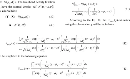
Y in order to obtain the value of xˆMMSE(y). However, analytical solution of these integrals is a hard and tedious task and certain numerical methods can be implemented. In the Fig. 7, xˆMMSE(y) is illustrated for
0 0 = =µ
µx in three cases of y=0,y<0, and y>0.
In Fig. 7, the lower surface illustrates the performance of the estimator of the Eq. 43 for y=0,and
, 0
σ σx,variations in the (0,1.5) range. As can be observed, when y=0, the estimation magnitude will be higher for an increase in σ0 orσx. When y≠0,
and σx is very small, the upper part of Fig. 7, the best
estimation will be equal to zero for all positive or negative observations. This result seems logical, because the infinitesimal value of σx will suggest a
deterministic behavior for the random variable X. However, for a great value of σx, there would be a
decrease in the estimation magnitude relative to observation when σ0increases. This is due to the fact that an increase in σ0, will result in an increase in the observations variance, and this causes the best estimation to be a very small value. For a high value of
0
σ , the same justification as σx can be implemented.
Table 4. Parameters of normal ECG signal in lead avr Events
Parameters
P Q R T
µ ij
t <sec>
8.75 8.89 8.92 9.14
ij
C <mV>
-0.2 -1.0 0.1 -0.3
ξ ij
t <sec> 0.1266 0.0448 0.0448 0.3250
Table 5. Parameters of normal ECG signal in lead V1
Events
Parameters
P R S T
µ ij
t <sec>
12.14 12.26 12.29 12.57
ij
C <mV>
-0.1 0.19 -1.11 -0.2
ξ ij
t <sec>
0.1036 0.0448 0.0822 0.2622
Table 6. Parameters of normal ECG signal in lead V3
Events
Parameters
P R S T
µ ij
t <sec>
8.45 8.61 8.64 8.83
ij
C <mV>
0.2 0.97 -2.04 0.81
ξ ij
t <sec>
0.1266 0.0448 0.0448 0.3921
Table 7. Parameters of normal ECG signal in lead V6
Events
Parameters
P Q R S T
µ ij
t <sec>
9.55 9.695 9.715 9.74 10
ij
C <mV>
0.05 -0.2 1.2 -0.4 0.5
ξ ij
t <sec>
0.1769 0.0291 0.0448 0.0448 0.2041
0 0.5
1 1.5
0 0.5
1 1.5
-1
-0.8
-0.6
-0.4
-0.2 0 0.2 0.4
σ σσ σ0
σ σσ σx E
sti ma te d V alu e
0 0.5
1 1.5
0 0.5
1 1.5
0 0.2 0.4 0.6 0.8 1
σ σσ σ0
σ σσ σ
x
E sti ma te d V alu e
0
0.5
1
1.5 0
0.5
1
1.5
-0.5 0 0.5 1 1.5 2 2.5 3
x 10-16
σ σ σ σ0
σ σσ σx E
sti ma te d V alu e
Fig. 7. Bayesian Estimation of the random variable X based on normal observation Y=ydescribes by Eq. (42) (up-left), y<0, (up-right), y>0 and (bottom), y=0
4 Simulation Results
The results of various simulations will be illustrated in this part.
4.1 15 Lead Normal ECG Generator (including Probable U-Waves)
First, the simulation method of generating 15-lead normal ECG signal with U-wave are presented. Some
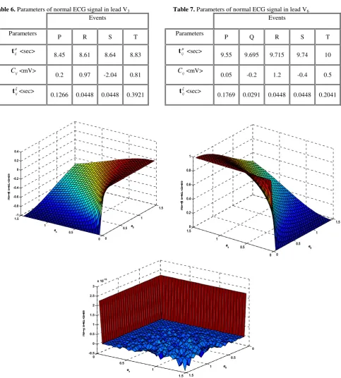
abnormal electrocardiographic phenomena are then simulated. In Figs. 8 to 11, a normal beat is shown in the leads AVR, V1, V3, and V6, respectively and the corresponding parameter values are presented in Tables 4 to 7. It should be noted that the lead AVR and V1 have no S-wave, and no Q-wave, respectively. However, the lead V6 contains all events. In Fig. 12, an
example of a heart beat with a U-wave is depicted and the corresponding parameters are represented in Table 8.
8.6 8.7 8.8 8.9 9 9.1 9.2 9.3
-1 -0.8 -0.6 -0.4 -0.2 0 0.2 0.4
time(sec) a
m plit u d e ( m V)
Fig. 8. Simulated normal ECG signal in lead avr
11.9 12 12.1 12.2 12.3 12.4 12.5 12.6 12.7 12.8
-1 -0.5 0 0.5
time(s) a
m plit u d e( mV )
Fig. 9. Simulated normal ECG signal in lead V1
8.3 8.4 8.5 8.6 8.7 8.8 8.9 9 9.1 9.2
-2.5
-2
-1.5
-1
-0.5 0 0.5 1
time(sec) a
m plir u d e( m V)
Fig. 10. Simulated normal ECG signal in lead V3
9.4 9.5 9.6 9.7 9.8 9.9 10 10.1
-0.4 0.1 0.6 1.1 1.4
time(sec) a
mpl it u de ( mV )
Fig. 11. Simulated normal ECG signal in lead V6
9.4 9.6 9.8 10 10.2 10.4
-0.4 -0.2 0 0.2 0.4 0.6 0.8 1
time(sec) a
m plit u d e( mV )
Fig. 12. Simulated normal ECG signal in lead I including U-wave
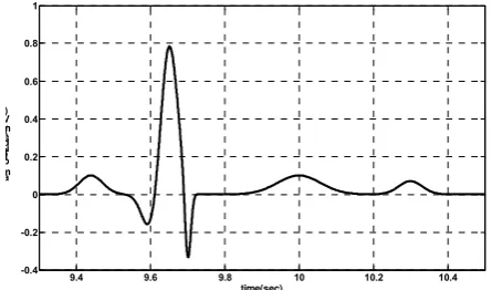
4.2 Fascicular Ventricular Tachycardia (Left Septal Ventricular Tachycardia)
A left septal Ventricular Tachycardia (VT) has been described as arising in the left posterior septum, often preceded by a fascicular potential, and is sometimes called a fascicular tachycardia (Fig. 13). The simulated abnormal left septal ventricular tachycardia waveforms are demonstrated in Figs. 14 to 17 and the corresponding parameter values are presented in Tables 9 to 12. The comparison of the
simulated waveforms and real shapes of
electrocardiographic signals (depicted in Fig. 13) indicates the high flexibility of the introduced model in generating artificial abnormal ECG waveforms.
Fig. 13. Left septal ventricular tachycardia. This tachycardia is characterized by a right bundle branch block contour. In this instance, the axis was rightward. The site of the ventricular tachycardia was established to be in the left posterior septum by electrophysiological mapping and ablation, adopted from [12]
0 5 10 15 20 25 30 35 40 45 50 55 -4
-2 0 2 4 6 8 10 12
time(sec) a
m plit u de ( mV )
(a)
0 5 10 15 20 25 30 35 40 45 50
0 5 10 15
time(sec) a
m plit u d e( mV )
(b)
0 5 10 15 20 25 30 35 40 45 50
0 1 2 3 4 5 6 7 8
time(sec) a
m plit u d e( mV )
(c)
Fig. 14. Simulated left septal ventricular tachycardia in leads (a) avf, (b) avl, and (c) avr
Table 8. Parameters of normal ECG signal in lead I including U-wave
Events
Parameters P Q R S T U
µ ij
t <sec> 9.44 9.6 9.65 9.7 10 10.3
ij
C <mV> 0.1 -0.2 0.8 -0.4 0.1 0.07
ξ ij
t <sec> 0.1769 0.1266 0.1266 0.0448 0.325 0.1769
Table 9. Parameters of left septal ventricular tachycardia in leads (a) avf, (b) avl, and (c) avr
Events
Parameters P Q R
µ ij
t <sec>
-0.5 3 3.5
ij
C <mV> 10 5 -5
ξ ij
t <sec> 5 6 7
(a)
Events
Parameters P Q R
µ ij
t <sec> 0 3 5.1
ξ ij
t <sec> 5 5 6
ij
C <mV> 2 7 0.8
(b) Events
Parameters P Q
µ ij
t <sec> 0 4.7
ξ ij
t <sec> 9 8
ij
C <mV> 10 8
(c)
0 5 10 15 20 25 30 35 40 45 0
2 4 6 8 10 12
time(sec) a
m plit u d e( m V)
(a)
0 10 20 30 40 50 60
-12 -10 -8 -6 -4 -2 0 2 4 6 8
time(sec) a
m plit u d e( mV )
(b)
0 10 20 30 40 50 60
-10
-8
-6
-4
-2 0 2 4 6 8 10
time(sec) a
m plit u d e( mV )
(c)
Fig. 15. Simulated left septal ventricular tachycardia in leads (a) I, (b) II, and (c) III
Table 10. Parameters of left septal ventricular tachycardia in leads (a) I, (b) II, and (c) III
Events
Parameters P Q
µ ij
t <sec> 0 5
ξ ij
t <sec> 9 8
ij
C <mV> 10 4.5
(a)
Events
Parameters P Q R
µ ij
t <sec> 0 1.75 3.8
ξ ij
t <sec> 3.5 5 7.4
ij
C <mV> 7 3 -12
(b) Events
Parameters P Q R
0 4 4.5
ξ ij
t <sec> 5.5 6 8
ij
C <mV> 7 2.3 -10
(c)
Table 11. Parameters of left septal ventricular tachycardia in leads (a) V1, (b) V2, and (c) V3
Events
Parameters P Q R
µ ij
t <sec>
-0.5 1.2 2.5
ξ ij
t <sec> 2.8 3 4
ij
C <mV> 2 8 10
(a)
Events
Parameters P Q R
µ ij
t <sec> -2 5 6
ξ ij
t <sec> 7 6 8
ij
C <mV> 5 12 -20
(b)
0 5 10 15 20 25 30 35 40 45 0
2 4 6 8 10 12
time(sec) a
m plit u de ( mV )
(a)
0 10 20 30 40 50 60 70
-20
-15
-10
-5 0 5 10 15
time(sec) a
mpl it u d e( mV )
(b)
0 10 20 30 40 50 60
-15
-10
-5 0 5 10 15
time(sec) a
m plit u d e( mV )
(c)
Fig. 16. Simulated left septal ventricular tachycardia in leads (a) V1, (b) V2, and (c) V3
0 5 10 15 20 25 30 35 40 45
-20 -15 -10 -5 0 5 10
time(sec) a
m plit u d e( mV )
(a)
0 10 20 30 40 50 60 70
-12 -10 -8 -6 -4 -2 0 2 4 6
time(sec) a
m plit u d e( mV )
(b)
0 10 20 30 40 50 60
-8
-6
-4
-2 0 2 4
time(sec) a
m plit u de ( m V)
(c)
Fig. 17. Simulated left septal ventricular tachycardia in leads (a) V4, (b) V5, and (c) V6
Table 12. Parameters of left septal ventricular tachycardia in leads (a) V4, (b) V5, and (c) V6
Events
Parameters P Q R
µ ij
t <sec> 0 1.2 4.5
ξ ij
t <sec> 3 5 6
ij
C <mV>
-20 10 7
(a)
Events
Parameters P Q R
µ ij
t <sec> -2 3 2.9
ξ ij
t <sec> 3.5 4 8
ij
C <mV> 5 2 -11
(b)
Events
Parameters P Q R
µ ij
t <sec> -1 3.5 4
ξ ij
t <sec> 5 5.5 8
ij
C <mV> 4 1.5 -8
(c)
4.3 Rate-Dependent Conduction Blocks or Aberration (Tachycardia, Bradycardia)
Conduction delays in the intra-ventricular parts can be due to changes in heart rate, or pathological lesions in the conduction system. Rate-dependent block (aberration) can occur in relatively low or high heart rates. A very pervasive kind of rate-dependent block which has the electrocardiographic pattern of Right Bundle Branch Block (RBBB) or Left Bundle Branch Block (LBBB) is called acceleration (tachycardia)-dependent block, in which conduction delay happens when heart rate exceeds a specific critical threshold. On the other hand, in deceleration (bradycardia)-dependent block conduction delay takes place when heart rate is less than the specific critical threshold. Deceleration-dependent block is less prevalent in comparison to acceleration-dependent block and only occurs in patients with remarkable defect in the conduction system.
In Fig. 18-a, a sample acceleration-dependent QRS aberration is depicted. As can be seen in this picture, the duration of the basic cycle, C is equal to 760 milliseconds, and left bundle branch block (LBBB) occurs when C reaches the value of 700 milliseconds, which is annotated by some points. The occurred block will then continue with the cycle duration of 700msec in Fig. above and 840msec in Fig. below, which is annotated by arrowheads. Eventually, the conduction system returns to its normal conditions after a heart beat with duration of 600msec. The beginning of each cycle with normal duration is illustrated by letter S, [12]. A simulated sample of this phenomenon is represented in Fig. 18-b. It should be noticed that three parameter sets will be required in this case which will apply to the points C, arrowhead, and S, which can be seen in Tables 13 to 15.
(a)
(b)
Fig. 18. (a) Electrocardiographic pattern of acceleration-dependent QRS aberration, adopted from [12], (b) the simulated signal with similar features
Table 13. parameters of acceleration-dependent aberration, phase I
Events
Parameters P Q R S S' T
µ ij
t <sec> 0.
2150
0. 3375
0. 3950
0. 4125
0. 5450
0. 7150
ij
C <mV> 0.
7
-0.4
0. 8
-0.7
0. 6
0. 6
ξ ij
t <sec> 0.
0850
0. 0375
0. 0650
0. 0375
0. 0850
0. 0850
Table 14. Parameters of acceleration-dependent aberration, phase II
Events
Parameters Q S T T'
µ ij
t <sec> 0.2950 0.4500 0.7100 0.7250
ij
C <mV> -0.8 -0.11 0.3 0.1
ξ ij
t <sec> 0.1050 0.050 0.1900 0.0750
Table 15. Parameters of acceleration-dependent aberration, phase III
Events
Parameters Q S S'
µ ij
t <sec> 0.2750 0.3500 0.4000
ij
C <mV> -0.6 -0.6 -0.8
ξ ij
t <sec> 0.0250 0.0500 0.1000
In Fig. 19-a, an example of deceleration-dependent aberration is presented. The basic rhythm is sinus rhythm with a Wenckebach (type I) atrioventricular (AV) block. With 1:1 AV conduction, the QRS complexes are normal in duration; with a 2:1 AV block
or after the longer pause of a Wenckebach sequence, left bundle branch block (LBBB) appears, [12]. A simulated sample of this phenomenon is represented in Fig. 19-b. It should be noticed that two parameter sets will be required in this case (see Tables 16 and 17).
(a)
(b)
Fig. 19. (a) Electrocardiographic pattern of deceleration-dependent aberration, [12]. (b) the simulated signal with similar features
Table 16. Parameters of deceleration-dependent aberration, phase I
Events
Parameters P Q R R' S
µ ij
t <sec> 0.
5
0. 55
0. 9500
1. 025
1. 3
ij
C <mV> 0.
02
-0.16
0. 02
0. 01
-0.01
ξ ij
t <sec> 0.
1
0. 0500
0. 3500
0. 0750
0. 1
Table 17. Parameters of deceleration-dependent aberration, phase II s
Events
Parameters P Q R S T
µ ij
t <sec> 0.
35
0. 625
0. 8000
1. 1500
1. 5000
ij
C <mV>
-0.1
0.
2 -2 1
0. 1
ξ ij
t <sec> 0.
1
0. 0750
0. 2000
0. 3500
0. 2000
4.4 Acute Q- Wave Infarctions of anteriorlateral and inferior walls
Approximate classification and variability of electrocardiographic patterns of acute myocardial ischemia are illustrated in Fig. 20. It should be noted that this classification cannot be applied to all cases. As a case in view, a Q-wave infarct can evolve to a Q-wave infarct and an ST-elevation can be developed by a
non-Q wave infarct. Reversely, ST- segment depression and T-wave inversion can occur by the happening of a Q-wave infarct, [12].
Fig. 20. A general classification, but not always accurate, of myocardial ischemia, Adopted from [13]
4.5 QRS Changes
Due to the existence of real infarctions, depolarization changes (QRS complexes) are always followed by abnormal repolarization (ST-T) [15, 24]. Necrosis of a rather large part of the myocardial tissue can lead to reductions in R-wave or Q-wave amplitude of anterior, lateral, or inferior leads. This can be a result of lack of electromotive forces in the infracted area. It was assumed in the past that abnormal Q-waves are markers of transmural myocardial infarction and subendocardial (transmural) infarctions do not make
Q-waves. However, profound studies of pathological electrocardiographic signals suggested that transmural infarcts can occur with no Q-wave, or subendocardial infarcts can be accompanied by Q-waves. Therefore, a better way for the classification of infarcts is to divide them into Q-wave and Non-Q wave infarcts, instead of transmural or non-transmural infarcts [12].
4.6 Evolution of Electrocardiographic Changes
Evolution of Electrocardiographic Changes in ischemic ST-elevation and hyper-acute T-wave changes serve as the first symptoms of acute infarction. In a time period of some hours to some days, these symptoms will be followed by T-wave inversion and sometimes Q-waves. In the state of chronic ischemia or evolutionary condition, T-wave inversion will somehow be related to
the long duration of the ventricular action potential and these ischemic changes are always followed by QT prolongation. After days or weeks, T-wave inversion will be resolved or will continue infinitely. The largeness of the infracted area is a good reflective of the quality of T-wave evolution (see Fig. 21). Transmural infarction with fibrosis of entire wall will exist, if T-waves have a negative value in the leads with a Q-wave. However, T-waves with a positive value in the leads with a Q-wave are a symptom of non-transmural infarction with workable myocardium of the wall [12]. The depolarization and repolarization change patterns are illustrated in Fig. 21 in the case of Q-wave infarction. Anterior-lateral infarcts will lead to ST-segment elevation in leads I, AVL, and pericardial leads which will be accompanied by ST-segment depression in the leads II, III, and AVF. On the other hand, acute inferior (or posterior) infarcts can be followed by reciprocal ST-segment depression in the leads V1 to V3. In Fig. 22, some selected samples of patterns depicted in Fig. 21 with different types of transient ST-segment episodes are simulated.
The corresponding parameter values for simulation of ST-T events during acute Q-wave infarction are presented in Table 18.
Noninfarction subendocardial ischemia (including classic angina)
Transient ST depressions
Non-Q-wave infarction
ST depressions or T-wave inversions without Q-waves
Myocardial Ischemia
Noninfarction transmural ischemia (including Prinzmetal
variant angina)
Transient ST elevation or paradoxical T-wave normalization,
sometimes followed by T-wave inversions
ST elevation Q-wave infarction
Approximate classification
and variability of
electrocardiographic patterns
Fig. 21. Sequence of electrocardiographic patterns of depolarization and repolarization changes during Q –wave infarction in the early and evolving regimes, (top): acute anterior- lateral and (bottom): acute inferior wall Q-wave infarctions, Adopted from [12]
(a) (b) (c) (d)
(e)
(f) (g) (h)
(i) (j) (k) (l)
(m)
(n) (o) (p)
Fig. 22. Simulated ST-T episodes during acute Q-wave infarction:
Acute anterior-lateral wall Q-wave infarction in early regime for (a) lead I, (b) lead V2, (c) lead V4, (d) lead V6
Acute anterior-lateral wall Q-wave infarction in evolving regime for (e) lead I, (f) lead V2, (g) lead V4, (h) lead V6
Acute inferior wall Q-wave infarction in early regime for (i) lead I, (j) lead V2, (k) lead V4, (l) lead V6
Acute inferior wall Q-wave infarction in evolving regime for (m) lead I, (n) lead V2, (o) lead V4, (p) lead V6
Table 18. The corresponding parameters for simulation of ST-T events during acute Q-wave infarction
Events Parameters AE1 AE2
µ ij
t <sec> 0.2500 0.3250
ij
C <mV> -0.02 0.02
ξ ij
t <sec> 0.0500 0.075
![Fig. 6. using artificial RR-tachogram generator introduced in [9] Modulation of QRS complexes based on Eq.s 17 to 19](https://thumb-us.123doks.com/thumbv2/123dok_us/217190.2016202/9.595.347.501.89.210/using-artificial-tachogram-generator-introduced-modulation-complexes-based.webp)