RESEARCH NOTE
A TIME-DOMAIN METHOD FOR SHAPE RECONSTRUCTION
OF A TARGET WITH KNOWN ELECTRICAL PROPERTIES
R. Alvandi* and M. Kamyab
Department of Electrical Engineering, K.N. Toosi University of Technology P.O. Box 16315-1355, Tehran, Iran
[email protected] - [email protected]
*Corresponding Author
(Received: October 29, 2006 – Accepted in Revised Form: May 9, 2008)
Abstract This paper uses a method for shape reconstruction of a 2-D homogeneous object with arbitrary geometry and known electrical properties. In this method, the object is illuminated by a Gaussian pulse, modulated with sinusoidal carrier plane wave and the time domains’ footprint signal due to object presence is used for the shape reconstruction. A nonlinear feedback loop is used to minimize the difference between the measured and calculated signals obtained, by using FDTD at consecutive time windows. The layers of the objects’ shape are reconstructed while the incident plane wave moves over the objects’ surface. Based on the above method, some results are presented for an object with typical geometry. The effect of modulating carrier frequency was investigated for conductivity and dielectric objects.
Keywords Inverse Scattering, FDTD, Causality, Plane Wave
ﻩﺪﻴﮑﭼ
ﻚـﻳﺮﺘﻜﻟﺍ ﻱﺩ ﻭ ﻚـﻳﺮﺘﻜﻟﺍ ﺐﺋﺍﺮـﺿ ﺎـﺑ ﻦﮕﻤﻫ ﻱﺪﻌﺑﻭﺩ ﻡﺎﺴﺟﺍ ﻞﻜﺷ ﻱﺯﺎﺳﺯﺎﺑ ﻱﺍﺮﺑ ﻲﺷﻭﺭ ﻪﻟﺎﻘﻣ ﻦﻳﺍﺭﺩ
ﺖﺳﺍ ﻩﺪﺷ ﻪﺋﺍﺭﺍ ﻡﻮﻠﻌﻣ .
ﺺﺨﺸﻣﺎﻧ ﻢﺴﺟ ﺵﻭﺭ ﻦﻳﺍ ﺭﺩ )
ﻑﺪﻫ ( ﻝﻭﺪـﻣ ﻲـﺳﻮﮔ ﺖـﺨﺗ ﺲﻟﺎﭘ ﻚﻳ ﺶﺑﺎﺗ ﺽﺮﻌﻣ ﺭﺩ
ﻲﻣ ﺭﺍﺮﻗ ﻩﺪﺷ
ﺎﺳﺯﺎﺑ ﻑﺪﻫ ﻞﻜﺷ ﻲﺑﺎﺗﺯﺎﺑ ﻝﺎﻨﮕﻴﺳ ﺭﺩ ﻩﺪﺷ ﺩﺎﺠﻳﺍ ﺕﺍﺮﻴﻴﻐﺗ ﺯﺍ ﻩﺩﺎﻔﺘﺳﺍ ﺎﺑ ﻭ ﺩﺮﻴﮔ ﻲﻣ ﻱﺯ
ﺩﻮـﺷ . ﻚـﻳ ﺭﺩ
ﻩﺯﺍﺪﻧﺍ ﺮﻳﺩﺎﻘﻣ ﻦﻴﺑ ﻱﺎﻄﺧ ﻲﻄﺧﺮﻴﻏ ﺭﻮﺧﺯﺎﺑ ﻪﻘﻠﺣ ﺵﻭﺭ ﻚـﻤﻛ ﻪﺑ ﻩﺪﺷ ﻪﺒﺳﺎﺤﻣ ﻭ ﻩﺪﺷ ﻱﺮﻴﮔ
FDTD
ﻩﺮـﺠﻨﭘ ﺭﺩ ، ﻱﺎـﻫ
ﻲﻣ ﻞﻗﺍﺪﺣ ﻪﺑ،ﻲﻟﺍﻮﺘﻣ ﻲﻧﺎﻣﺯ
ﻪﻳﻻ ﺕﺭﻮﺻ ﻪﺑ ﻑﺪﻫ ﻞﻜﺷ ﻭ ﺪﺳﺭ ﻤﻫ ،ﻱﺍ
ﺰ ﻱﺯﺎـﺳﺯﺎﺑ ﻥﺁ ﻞـﺧﺍﺩ ﺯﺍ ﺝﻮﻣ ﺖﻛﺮﺣ ﺎﺑ ﻥﺎﻣ
ﻲﻣ ﺩﻮﺷ .
ﺳ ﺎﺑ ﻲﻓﺍﺪﻫﺍ ﻞﻜﺷ ﻱﺯﺎﺳﺯﺎﺑ ﺯﺍ ﻪﻠﺻﺎﺣ ﺞﻳﺎﺘﻧ ﻲﺧﺮﺑ
ﺖـﺳﺍ ﻩﺪـﻣﺁ ﻪﻟﺎﻘﻣ ﻦﻳﺍ ﺭﺩ ،ﻲﻋﻮﻧ ﻊﻄﻘﻣ ﺢﻄ .
ﻦﻴـﻨﭽﻤﻫ
ﺎﺳﺯﺎﺑ ﺖﺤﺻ ﺮﺑ ﻲﺸﺑﺎﺗ ﻊﺒﻨﻣ ﻥﻮﻴﺳﻻﻭﺪﻣ ﺲﻧﺎﻛﺮﻓ ﺮﻴﺛﺎﺗ ﺯ
ﻲﺳﺭﺮﺑ ﻱ ﺪﺷ
ﺖﺳﺍ ﻩ .
1. INTRODUCTION
Electromagnetic inverse scattering is a method in which an object whose geometry and/or electrical properties is unknown and also illuminated by electromagnetic waves and also the unknown characteristics of the object is estimated, by analyzing the measured scattered field. This method can be applied in cases that the object is located somewhere far away from the observer and the visual inspection is not possible. So this method can be a useful technique for developing a remote sensing for different kinds of imaging in various sciences and running non-destructive test on dissimilar structures.
For solving inverse scattering problem, some approximations are usually considered such as ignoring diffraction effect or multiple scattering, although there are methods which calculate the exact solution. The word “exact” means that all diffraction and multiple scattering effects are included in the calculations and errors in the solution will arise solely due to numerical approximations such as discretization and round-offs [1].
Trial target shape FDTD
code Nonlinear shape
optimization
measured i
E
FDTD i
E e
Reconstructed target shape
h
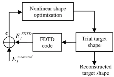
Figure 1. Block diagram of FDTD/feedback loop.
entire medium with the incident field is considered simultaneously. For a general, inhomogeneous medium those are lost, can result in a very large number of unknown parameters, which usually ensures using approximations. In contrast, time domain approaches, can use causality to limit the region of inversion, potentially reducing the number of unknowns [2].
For estimating the shape of an object, this paper aims to use, the time domain footprint signal of the object. This method reported by Umashankar, et al [1]. Assuming that the electrical properties of the object is known, the method uses a feedback loop to minimize the difference between the measured signal and the calculated signal obtained by using FDTD at consecutive time windows and reconstructs the layers of the objects’ shape while the incident wave passes through the object. The method is based on the causality principle. Using causality makes it possible to reconstruct the shape of the target simultaneously while the incident field moves on the target surface in consecutive time steps. A Gaussian pulse modulated with sinusoidal carrier was used as exiting source, and the effect of modulating carrier frequency was investigated for conductivity and dielectric objects. It will show that the carrier frequency doesn’t have any effect on conducting object reconstruction. The effect, on dielectric object reconstruction however is very significant, in particular at frequencies near resonance of the target; as well as at very low frequencies. Also the linear zone relative to observation point, clarified. The layer reconstruction, in this zone has correct answer.
2. OPTIMIZATION LOOP
Figure 1 shows a block diagram of the basic shape optimization loop. The FDTD forward scattering code calculates the pulse response of a trial target subjected to plane wave illumination. The pulse response computed by FDTD at the observation point is then compared with the measured pulse response, and an error signal is generated. This error signal is fed into a shape optimization routine which perturbs the trial target in a way that reduces the difference between the FDTD trial response and the measured pulse response in the least-square sense. We minimize error term given by:
| FDTD i E N
1 n
measured i
E |
e ∑
= −
= (1)
Where Eimeasured the set of is measured samples of the pulse response at the observation point and
FDTD i
E is the set of time samples of the pulse response computed by the forward scattering FDTD block [2].
3. CAUSALITY LOCUS
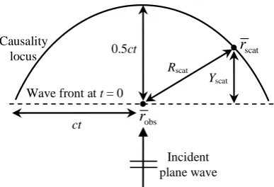
Figure 2 shows the movement of causality locus in two-dimensional free space after passing time t. In fact, causality explains that the locus of those points which can be considered as scatterer edge must satisfy the following formula:
ct scat R scet
Y + = (2)
Let us suppose that the first part of scattered wave is received in the observation point at time t0. The
causality locus in considered space is drawn on the basis of time t0. The first scattering point, which is
Causality locus
ct
Wave front at t = 0 0.5ct
Rscat Yscat
scat r
obs r
Incident plane wave
Figure 2. Free space causality locus at time t.
0 10 20 30 40 50 60 70 80
0 10 20 30 40 50 60 70 80
x*dx(meter)
y*
d
y
(m
e
ter)
causality locus
Figure 3. Causality locus movement in free space without presence of scatterer.
(a) (b) (c)
Figure 4. The target shape observed from different sides.
After locating the first point, we reconstruct the target sequentially in time as the causality locus moves across the target. The main advantage of causality locus is that, in a certain time, the partial shape of the target which is placed under causality locus would be reconstructed. Therefore, the complicacy of shape reconstruction would decrease and since it is considered a homogeneous object, its edges can be reconstructed.
4. LAYER RECONSTRUCTION
Figure 3 shows the way of causality locus movement in free space without the presence of scatterer. The source is a plane wave which is propagating in the +y direction. The observation point is located at x = 40 m and y = 10 m. In Figure 4, it can be seen that, as the causality locus goes far away from the observation point, it can be approximated as direct line in that part of space which is marked in the figure. This fact simplifies solving the inverse scattering problem.
If there is a target in a considered space that does not have reentrant features, the above approximation still holds. According to marked space in Figure 3, it is obvious that for more accuracy, the observation point should be far away from big objects.
This approximation helps one to reconstruct the target in layers. In fact, we can reconstruct the shape of target as a series of parallel layers. Thickness of each layer is determined according to the position of the causality locus toward previous layer. Optimization program must be able to find out the thickness of new layer and its position in comparison with previous layer which is already added.
5 10
15 20 0
5 10
15 20
25 0
0.1 0.2 0.3 0.4 0.5
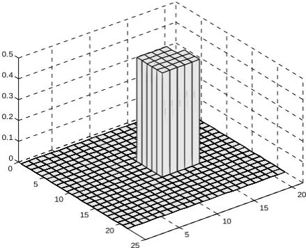
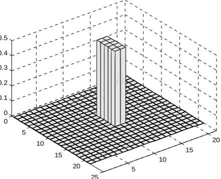
Figure 5. The reconstructed shape for the side (a) of the target shown in Figure 4.
5 10
15 20 0
5 10
15 20
25 0
0.1 0.2 0.3 0.4 0.5
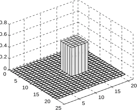
Figure 6. The reconstructed shape for the side (b) of the target shown in Figure 4.
About dielectric targets, it should be noticed that electromagnetic wave can enter the target, so the round trip speed of wave in each layer, is affected by dielectric permittivity. In fact, just considering the dielectric permittivity of the target for calculation of the optimum time window is not enough and the reconstruction of the target shape will include error. It seems that in addition to dielectric permittivity, other factors such as frequency and the shape of previous layers have effects on multiple scattering and consequently scattered waves, so it needs more accuracy in choosing optimum time window. Because of this fact, for reconstruction of dielectric targets, some changes must be done in the program and in reconstruction of each layer, the best time window is chosen accordingly.
5. RESULTS
In this section, the results are presented for a conductive target which is illuminated by a plane wave from different directions. In other word, the target is observed from different angles (Figure 4). In all presented results, the incident wave is a TM-polarized modulated by a Gaussian pulse carrier burst 5 cycles long. The frequency is 3GHz and the observation point is located at 0.5 λ0 from the front
edge of the target. The space of the simulated area is discretized into 80 × 80 square cells. The spatial resolution of shape reconstruction is as the FDTD code resolution and equals 1mm (= λ0/100). The
reconstructed shapes for different sides of the target have been presented in Figures 5-7. It is noted that for better visualization of the reconstructed shapes, the distance between the target and the observation point has not been shown in the presented figures.
There is a slight difference between the reconstructed shape shown in Figure 6 and its exact counterpart. In this case, the target is observed from an angle for which the target variations are not visible to the observer. The reconstruction error is due to the fact that the target variations lies in the shadow region and the variation is relatively high. It is noted that the same results are obtained for a dielectric target with the shape depicted in Figure 4.
6. EFFECTS OF MODULATION FREQUENCY ON SHAPE
RECONSTRUCTION
5 10
15 20 0
5 10
15 20
25 0
0.1 0.2 0.3 0.4 0.5
Figure 7. The reconstructed shape for the side (c) of the target shown in Figure 4.
5 10
15 20 0
5 10
15 20
25 0
0.1 0.2 0.3 0.4 0.5
Figure 8. The reconstructed shape at f = 300 MHz.
5 10
15 20 0
5 10
15 20
25 0
0.2 0.4 0.6 0.8
Figure 9. The reconstructed shape at f = 3 GHz, 6 GHz and 10 GHz.
the edges of the considered target are approximately smooth, the causality locus in the space is linear; and no problem will happen in reconstruction. In addition, no approximation which is related to frequency has been used for solving the problem, and the target shape is reconstructed accurately.
In reconstruction of dielectric targets, since wave enter the target, the selection of the modulated frequency is important in low frequencies for which the dimension of the target is much smaller than the wavelength. In this case, electromagnetic fields inside the target are semi-static and do not have any wavy properties, so scattering fields do not contain needed information. Therefore the correct reconstruction of the shape is not possible. In addition, if the frequency is increased so that the target dimension is an integer multiples of λ/4, an intensive resonance takes place inside the target and scattering fields does not provide correct information for reconstruction.
In presented example, a dielectric square with dimensions 5 mm × 5 mm and εr = 4 is placed
50mm far from observation point. The radiated pulse is modulated with 300 MHz, 3 GHz, 6 GHz, 10 GHz, 15 GHz, and 30 GHz whose associated wavelengths are respectively, 1 m, 0.1 m, 0.05 m, 0.03 m 0.02 m and 0.01 m. The results of reconstruction are shown in Figures 8-10. At
frequency of 300 MHz for which λ = 1 m and at frequencies of 15 GHz and 30 GHz for which the dimensions of target are about λ/2 and λ/4, the results of reconstruction are not correct.
7. CONCLUSIONS
5 10
15 20 0
5 10
15 20
25 0
0.1 0.2 0.3 0.4 0.5
Figure 10. The reconstructed shape at f = 15 GHz and 30 GHz.
due to the object scattering. The main advantage of this method is its good speed in shape reconstruction. Also, the method is based only on the backscatter footprint signal, whose measurement procedure is simpler, with respect to those methods which need bi-static radar cross sections. Furthermore, in reconstructing the shape of the target, all effects arising from wave scattering in space, such as diffraction and multiple scattering are considered, so the answer is precise.
It was shown that the frequency of modulating carrier is significant in case of dielectric target, but has no effect on the reconstruction of conductor object.
The presented method can also be used for
reconstruction of three-dimensional targets. For example, if the target excited by a point source, the causality locus will change into a causality surface which has a spherical movement in the free space. If the target is far away from the source, the spherical surface is approximately planar and the target can be reconstructed layer by layer. The presented method can be combined with other optimization algorithms such as genetic algorithm to estimate the shape and the electrical properties of the target at the same time.
8. ACKNOWLEDGMENT
The authors acknowledge the research grant provided by Telecom Research Center of Iran, which consequently made this paper possible.
9. REFERENCES
1. Yagle, A. E. and Frolik, J. L., “On the Feasibility of Impulse Reflection Response Data for the Two-Dimensional Inverse Scattering Problem”, IEEE Transactions on Antennas and Propagation, Vol. 44, No. 12, (1996).
2. Popovic, M. and Taflove, A., “Two-Dimensional FDTD Inverse Scattering Scheme for Determination of Near-Surface Material Properties”, IEEE, Vol. 1, (2003), 523-526.
3. Strickel, M., Taflove, A. and Umashankar, K., “Finite-Difference Time Domain Formulation of an Inverse Scattering Scheme for Remote Sensing of Conducting and Dielectric Target: Part 2-Two Dimensional Case”,