Optimization of Meshless Local Petrov-Galerkin Parameters using Genetic Algorithm for 3D Elasto-static Problems (TECHNICAL NOTE)

TECHNICAL NOTE

OPTIMIZATION OF MESHLESS LOCAL PETROV-GALERKIN

PARAMETERS USING GENETIC ALGORITHM FOR 3D

ELASTO-STATIC PROBLEMS

A. Bagheri*, R. Ehsany and M.J. Mahmoodabadi

Department of Mechanics, Guilan University P.O. Box 3756, Rasht, Iran

[email protected] - [email protected] - [email protected]

G.H. Baradaran

Department of Mechanics, Shahid Bahonar University P.O. Box 76175-133, Kerman, Iran

[email protected]

*Corresponding Author

(Received: July 19, 2010 – Accepted in Revised Form: April 23, 2011)

Abstract A truly Meshless Local Petrov-Galerkin (MLPG) method is developed for solving 3D elasto-static problems. Using the general MLPG concept, this method is derived through the local weak forms of the equilibrium equations, by using a test function, namely, the Heaviside step function. The Moving Least Squares (MLS) are chosen to construct the shape functions. The penalty approach is used to impose essential boundary conditions. The complete study of the effects of radius of support domain on the accuracy and efficiency of the solution is performed. The values of this parameter leave a great effect on runtime and accuracy. The Genetic Algorithm (GA) is used to determine the optimum values of this MLPG parameter to minimize the runtime and maximize the accuracy. Several numerical examples are included to demonstrate that the present method is very promising for solving the elasto-elastic problems.

Keywords Meshless Local Petrov-Galerkin (MLPG), Moving Least Squares (MLS), Genetic Algorithm (GA), Optimization

هﺪﯿﮑﭼ شور ﻣﻮﺑ ﯽ نوﺪﺑ ﺶﻣ وﺮﺘﭘ -ﮐﺮﻟﺎﮔ ﯿ ﻦ

(MLPG)

اﺮﺑ ي ﻞﺣ ﻞﺋﺎﺴﻣ ﻮﺘﺳﻻا -ﺗﺎﺘﺳا ﯿ ﮏ ﻪﺳ ﺪﻌﺑ ي ﻪﺑ ﺘﺳرد ﯽ ﻪﺑ رﺎﮐ ﻪﺘﻓﺮﮔ ﺪﺷ . ﺎﺑ رد ﺮﻈﻧ ﻦﺘﻓﺮﮔ مﺮﻓ ﻠﮐ ﯽ MLPG ، اﯾ ﻦ شور زا ﺑﯿ ﻦ مﺮﻓ ﺎﻫ ي ﺿ ﻌﯿ ﻒ ﻣﻮﺑ ﯽ زا تﻻدﺎﻌﻣ ﻟدﺎﻌﺗ ﯽ جاﺮﺨﺘﺳا دﺮﮔ ﯾﺪ . اﯾ ﻦ شور ﺎﺑ هدﺎﻔﺘﺳا زا ﻊﺑﺎﺗ ﺎﻣزآ ﯾ ﺸ ﯽ ﻪﺑ مﺎﻧ ﻊﺑﺎﺗ ﻪﻠﭘ ا ي ﻮﻫ ﯾ ﺎﺴ ﯾﺪ درﻮﻣ ﺳرﺮﺑ ﯽ راﺮﻗ ﺖﻓﺮﮔ . شور ﻞﻗاﺪﺣ ﺮﻣ تﺎﻌﺑ كﺮﺤﺘﻣ

(MLS)

اﺮﺑ ي ﻦﺘﺧﺎﺳ ﻞﮑﺷ ﻊﺑاﻮﺗ بﺎﺨﺘﻧا دﺮﮔ ﯾﺪ . شور ﺘﻟﺎﻨﭘ ﯽ اﺮﺑ ي لﺎﻤﻋا اﺮﺷ ﯾ ﻂ زﺮﻣ ي مزﻻ هدﺎﻔﺘﺳا ﺪﺷ . ﻪﻌﻟﺎﻄﻣ ي ﻠﻣﺎﮐ ﯽ ورﺮﺑ ي تاﺮﺛا عﺎﻌﺷ ﻪﻨﻣاد ي ﺘﺸﭘ ﯿ ﻧﺎﺒ ﯽ ﺮﺑ ور ي ﺖﻗد و هدزﺎﺑ ﻞﺣ ترﻮﺻ ﺬﭘ ﯾ ﺖﻓﺮ . دﺎﻘﻣ ﯾﺮ اﯾ ﻦ ﺎﻫﺮﺘﻣارﺎﭘ ﺛﺎﺗ ﯿﺮ زﯾ دﺎ ي ﺮﺑ ور ي نﺎﻣز ﻞﺣ و ﺖﻗد ﺖﺷاد . رﻮﮕﻟا ﯾ ﻢﺘ ﺘﻧژ ﯿ ﮏ اﺮﺑ ي ﻪﺒﺳﺎﺤﻣ ي دﺎﻘﻣ ﯾﺮ ﻬﺑ ﯿ ﻪﻨ ي ﺎﻫﺮﺘﻣارﺎﭘ ي MLPG ﻪﺑ رﺎﮐ ﻪﺘﻓﺮﮔ ،ﺪﺷ ﺎﺗ نﺎﻣز ﻠﻤﻋ ﯿ تﺎ ار ﺶﻫﺎﮐ و ﺖﻗد ار اﺰﻓا ﯾ ﺶ ﺪﻫد . ﻨﭽﻤﻫ ﯿ ﻦ ﺪﻨﭼ ﯾ ﻦ لﺎﺜﻣ دﺪﻋ ي اﺮﺑ ي تﺎﺒﺛا ﻣاﯿ ﺶﺨﺑﺪ ندﻮﺑ شور ﺮﮐذ دﺮﮔ ﯾ هﺪ اﺮﺑ ي ﻞﺣ ﻞﺋﺎﺴﻣ ﻮﺘﺳﻻا -ﺗﺎﺘﺳا ﯿ ﮏ ﺑﯿ نﺎ هﺪﺷ ﺖﺳا . 1. INTRODUCTION

Compared with the Finite Element Method’s (FEMs) convenience and flexibility in use, it has been plagued for a long time, with the inherent problems such as locking, poor derivative solutions, etc... It is a well known fact that the accuracy of the FEM relies on the quality of the

contrast, the truly meshless local Petrov-Galerkin (MLPG) approach has become very attractive as a very promising method for solving 3D problems. The main advantage of this method over the widely used finite element methods is that it does not need any mesh, either for the interpolation of the solution variables or for the integration of the weak forms. The many researches in solving PDEs demonstrate that the MLPG method, and its variants, has become some of the most promising alternative methods for computational mechanics. Unfortunately, most researches are restricted to solving 2D problems. It is more challenging to apply the MLPG for solving 3D problems, because of the difficulty in handling the local integrals over the intersection of the local test function domain and the global boundary of the arbitrary 3D solution domain.

The MLPG method has been demonstrated to be quite successful in solving various partial differential equations. The MLPG concept was presented first by Atluri, et al [1]. They solved the elasto-static problems in two dimensional domains. Lin, et al [2] introduced an up winding scheme to analyze the steady state convection–diffusion problems. Liu, et al [3]coupled the MLPG method with either the finite element or the boundary element method to enhance the efficiency of the MLPG method. Ching, et al [4] augmented the polynomial basis functions with singular fields to determine deformations and stress fields near the crack tip for generally 2D mixed-mode problems. Gu, et al [5]and Batra, et al [6] used the Newmark family of methods to analyze 2D transient elasto-dynamic problems. The bending of a thin plate has been studied by Gu, et al [7] and Long, et al [8]. Although several research successes in solving boundary value problems in two dimensional domains illustrate that the MLPG method and its variants are much comparative with the Galerkin finite element method, there are only few works that study the application of MLPG methods in 3D problems. Han, et al [9] used the MLPG approach for solving the 3D problems in elasto-statics. They also applied the MLPG method in 3D elastic fracture [10] and 3D elasto-dynamics problems [11]. The MLPG method in the present study employs a Local Symmetric Weak Form (LSWF), the MLS approximation as the shape function and the Heaviside step function as the test function.

Although the MLS approximations have some drawbacks in dealing with the essential boundary conditions, they can be straightforwardly applied to 3D cases. One of the major advantages of the MLS is that, the shape functions are constructed from the local points only, with the high order continuities. Hence, this method leads to less cost in assembling the system equations.

In the general MLPG approach, the local test domains can be selected arbitrarily. Those are such as spheres, cubes, and ellipsoids in 3D domains. However, the local sub-domains become very complicated, for the points which are located on, or near the global boundaries. It happens because of the complicated intersection between the simple sub-domain and the boundary surfaces. In the present study, a method is developed to define the local sub-domains as spheres, with the use of a transformation which maps a circle on a semi-sphere for numerical integrations.

In this paper, the effects of radius of support domain are analyzed. Considering several examples and using the genetic algorithm, the optimum value of this parameter for the minimum computation time and the highest accuracy has been determined.

2. THE MOVING LEAST SQUARES (MLS)

The MLS method of interpolation is generally considered to be one of the best schemes to interpolate random data with a reasonable accuracy. Although the nodal shape functions that arise from the MLS approximation have a very complexnature,they always preserve completeness up to the order of the chosen basis, and robustly interpolate the irregularly distributed nodal information. The MLS scheme has been widely used in domain discretization methods. With the MLS, the distribution of function u in Ωx can be approximated as,

u(x) = pT(x)a(x) ∀x∈Ω_x (1)

where pT(x) = [p1(x),P2(x), ... ,

p

m(x)] is a monomial

monomial basis. They are determined by minimizing a weighted discrete L2 norm, defined, as:

] ˆ ) ( [ ] ˆ ) ( [ 2 ] ˆ ) ( ) ( )[ ( 1 ) ( u Pa W u Pa a P − − = − ∑ = = x T x i u x i x T x N i i w x J (2)

where

w

_i(x) is the weight function associated with the node i, N is the number of node in Ωx and uˆi

is the fictitious nodal value respective to node i. The matricesPand W are defined as:

matrix m N N x m p N x p N x p x m p x p x p x m p x p x p ) ( ) ( ... ) ( 2 ) ( 1 . . . ) 1 ( ... ) 2 ( 2 ) 2 ( 1 ) 1 ( ... ) 1 ( 2 ) 1 ( 1 × =                   = P (3)

( )

( )

matrix diagonal N N x N w x w ) ( . . . 0 . . . . . . . . . 0 . . . 1 × =                 = W (4) and

(

N

)

Vecto

N u u u

T _{= ×}

  



= ˆ1,ˆ2,..., ˆ 1 ˆ

u ₍₅₎

The stationary of J in Equation 2, with respect to

a(x) leads to the following linear relation between

a(x) and

u

ˆ

,

A(x)a(x) = B(x)

u

ˆ

(6) where matrices A(x)and B(x) are defined by

( )

( )

∑

( )

=            = = = N I I x T I x x I w x T x 1 p p P B WP P

A (7)

( )

( )

( )

( )

_               =

= T w x x w x x w_N x x_N

x P W p p p

B _{1 1} , _{2 2} ,...,

(8) when the coefficients a(x) in Equation 6 are determined, one may obtain the approximation

from the nodal values at the local scattered points, by substituting them into Equation 1, as:

u

Φ ( )ˆ

)

(x T x

u = (9)

where Φ(x) is the so-called shape function of the MLS approximation, defined as:

) ( ) ( 1 ) ( )

(x pT x A x B x

Φ = − (10)

The weight function in Equation 2 defines the range of influence of node i. Numerical practices show that a quadratic spline weight function works well [1,2]. Hence in this article, the quadratic spline weight function is used. Thus we have

( )

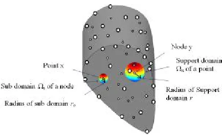
           ≥ ≤ ≤         −         +         − = i r i d i r i d i r i d i r i d i r i d x i W 0 0 4 3 3 8 2 6 1 (11) where di is the distance between points x and node

xi. ri is the size of support (see Figure 1) for the weight functions. It can be seen that the quadratic spline weight function C1 is continuous over the entire domain.

3. LOCAL SYMMETRIC WEAK FORMS (LSWF) OF 3D ELASTO-STATIC

PROBLEMS

Consider a linear elastic body in a 3D domain Ω, with a boundary ∂Ω (Figure 2). The solid is assumed to undergo infinitesimal deformations. The equilibrium equations are as follows:

i i ji ij i f j

ij σ σ _ξ

σ ∂ ∂ ≡ = =

+ 0, and ()_,

, (12)

Where σij is the stress tensor which corresponds

to the displacement field uiand fi is the body

force. The corresponding boundary conditions are given as follows,

i u i

Figure 1. Schematics of the MLS approximation.

Figure 2. Sub domain of a point and support domain of a nod.

i t j n ij i

t =σ = on Γ_t (13) where ui and ti are the prescribed displacements

and tractions, respectively, on the displacement boundary Γu and the traction boundary Γt; ni is the

unit outward normal to the boundary Γ (Figure 1). The strain-displacement relations are:

) , , ( 2 1

k l u l k u

kl = +

ε (14)

The constitutive relations of isotropic linear elastic homogeneous solid are:

l k u ijkl E kl ijkl E

ij= ε = ,

σ (15)

where

) ( _{ik jl il jk}

kl ij ijkl

E =λδ δ +µδ δ +δ δ (16)

with λ and µ being the Lame’s constants.

A generalized local weak form of the differential Equation 12 over a local sub-domain Ω_s can be written as:

0 )

( , + Ω=

∫

Ωs f vd

i i j ij

σ (17)

where ui and vi are the trial and test functions,

respectively. By applying the divergence theorem and the boundary conditions, Equation 17 may be rewritten in a symmetric weak form as:

∫Ω − Ω=

−

∫Γ Γ+∫Γ Γ

+

∫ Γ

s ijvi j fivi d

sutivid sttivid s

L tivid

0 ) ,

(σ (18)

where Γsu is a part of the boundary ∂Ωs of Ωs,

over which the essential boundary conditions are specified. In general, ∂Ωs =ΓsULs with

Γ

s being

a part of the local boundary located on the global boundary and L_s being the other part of the local boundary which is inside the solution domain.

u s

su =Γ Γ

Γ I is the intersection between the local boundary ∂Ωs and the global displacement

boundary

Γ

u. Γst=ΓsIΓt is a part of the boundary

over which the natural boundary conditions are specified.

Therefore, a local symmetric weak form (LSWF) in linear elasticity can be written as:

∫Ω Ω

+

∫Γ Γ=∫Γ Γ

−

∫ Γ

− Ω ∫Ω

s fivid sutivid sttivid

s L tivid d

j i v ij s(σ , )

(19)

If a Heaviside step function is used as the test function for the nodes on the natural boundary or inside the domain, i.e. su

I i

u

( )

∉

Γ

, one may simplify Equation 19 for

u

i(I) as:

∫Ω Ω

+ ∫Γ Γ=∫Γ Γ −

∫ Γ

−

s fid sutid sttid

s

L tid (20)

∫Ω Ω +

Γ ∫Γ +

∫Γ Γ+ ∫Γ Γ=∫Γ Γ −

∫ Γ

−

s fid d

suui

sutid suuid sttid s

L tid

α

α

(21)

In this equation coefficient

α

>>1 is used to impose essential boundary conditions.

The shape of sub domains in this study is chosen spherical and for numerical integrations, we use a transformation which maps a circle on a semi-sphere.

4. MULTI-OBJECTIVE OPTIMIZATION

Multi-objective optimization which is also called multicriteria optimization or vector optimization has been defined as finding a vector of decision variables satisfying constraints to give acceptable values to all objective functions [12]. In general, it can be mathematically defined as:

Find the vector

T n

x x x

X*={ ₁*, *₂,..., *} (22) to optimize

T

X k f X f X f X

F( )={ ₁( ), ₂( ),..., ( )} (23) subjected to m inequality constraints

m t

X i

g( )≤0 =1,2,..., (24) and

p equality constraints

p j X

h_i( )=0 =1,2,..., (25)

where n

R

X*∈ _{is the vector of decision or design} variables, and _F(X)∈Rn _{is the vector of objective} functions each of which are to be minimized or maximized. However, without loss of generality, it is assumed that all objective functions are to be minimized. Such multi-objective minimization based on Pareto approach can be conducted using some definitions [13]:

4.1. Definition of Pareto Dominance

A

vector U=[u₁,u₂,...,u_n], is dominant to vector

] ,..., , [v1 v2 vn

V = (denoted by U pV ) if and only if:

{

k

}

u_i v_i j

{

k

}

u_i v_j

i∈ ≤ ∧∃ ∈ <

∀ 1,2,..., , 1,2,..., : (26)

4.2. Definition of Pareto Optimality

A point

Ω ∈

*

X ₍Ω is a feasible region in n

R satisfying Equations 24 and 25) is said to be Pareto optimal (minimal) if and only if there is not X∈Ω which can dominate to *

X . Alternatively, it can be readily restated as:

) ( ) ( : } ,.. 2 , 1 { ,

, * *

X f X f k i

X X

X∈Ω ≠ ∃ ∈ _i < _i

∀ (27)

4.3. Definition of Pareto Set

For a given multi-objective optimization problem (MOP), a Pareto set

P

* is a set in the decision variable space consisting of all the Pareto optimal vectors

)} ( ) ' ( : ' {

* X X F X F X

P = ∈Ω ∋/ ∈Ω < (28)

4.4. Definition of Pareto Front

For a given MOP, the Pareto front *

PT is a set of vector of objective functions which are obtained using the vectors of decision variables in the Pareto set

P

* that is:

( )

( ) ( )

( )

   



 _∈

  

 =

= _{,..., :} *

2 , 1

* _{X X P}

k f X f X f X F PT

(29) In other words, the Pareto front _PT* _{is a set of} vectors of objective functions mapped from _P*_. Evolutionary algorithms have been widely used for multi-objective optimization because of their natural properties suited for these types of problems. This is mostly because of their parallel or population-based search approach. Most of the issues that exist in conventional methods are solved in these algorithms. For example, we can gain most of optimal decision vectors with a single run. But, in other methods we usually achieve only one in each run.

Genetic algorithm is one of the evolutionary algorithms. It uses direct values of functions and does not need to function’s derivations. These and other properties of GA caused its comprehensive use in optimization problems [13].

been recently used in a wide area of engineering MOPs because of its simple yet efficient non-dominant ranking procedure in yielding different level of Pareto frontiers [15,16]. In this paper modified NSGAII algorithm as a MO tool searches for the definition space of decision variables and returns the optimum answers in Pareto form [17].

5. MULTI-OBJECTIVE OPTIMIZATION OF MLPG ANALYSIS

The vector [r] is the vector of selective parameter of MLPG analysis (r is the support domain radius). The amount of runtime and error of the analysis, are functions of the components of this vector. This means that by selecting various values for the selective parameters, we can make changes in the amounts of runtime and error of MLPG analysis. In this paper, we are concerned with choosing the value of the selective parameter to minimize the two functions, the amount of runtime and error of the analysis. Clearly this is an optimization problem with two objective functions (runtime and error), and a decision variable (r). To solve this problem, we can make use of single-objective-optimization (SOO) or multi-objective single-objective-optimization (MO) algorithms.

When using SOO, we must exchange the multiple objective functions into one (using weight coefficients). Designer must decide about weight coefficients for all objective functions in proportion to optimality importance of each of them. So, the algorithm returns a single answer corresponding to weight coefficients. As compared with SOO, MO’s results are more complete and flexible. In a single run, MO returns a Pareto set of answers which includes all SOO’s answers too.

A Pareto set is a set of predominant answers which are non-dominated to each other (not having any dominance to each other). This means that we cannot find two members of this set that one is better than the other with respect to all of the objective functions. A Pareto set of answers presents possible different states to which optimal answers can be achieved with respect to their objective functions. It shows the condition of confrontation among objective functions and the way they vary from answer to answer.

As a result, designers by considering the

interaction among objective functions can haggle over their optimality. So, they can select an optimum and multipurpose answer consciously. In this paper, we used MO to find the selective parameters.

The aim of optimization in this section is finding the selective parameter of MLPG analysis to minimize the error and runtime of the analysis. Decision variable and its region are:

r: Support domain radius and (0 ≤ r ≤ (maximum distance between two nodes)) Constraints considered in the analysis are non singularity of matrix A(X) and global stiffness matrix. We use penalty functions to operate constraints. To do this, those objective functions of design vectors which violate the constraints are set as infinity, to be removed from the cycle in evolution process.

6. RESULTS OF NUMERICAL EXAMPLES

In this section, the meshless local Petrov–Galerkin method is applied to solve three-dimensional elasto-static problems. Two problems in three-dimensional linear elasticity are solved to illustrate the effectiveness of the present method. Numerical results are discussed consequently.

Example 1

In this case a cube under the hydrostatic pressure is considered. The MLPG approach is applied for this elasto-static problem with boundary conditions presented in Figure 3as

0

= = =

− = = =

τ τ τ

σ σ σ

z y x

p z y x

(30)

The analytical solutions for this problem are:

z p u z

b y p u y

a x p u x

µ λ

µ λ

µ λ

2 3

) 2 ( 2 3

) 2 ( 2 3

+ − =

− + − =

− + − =

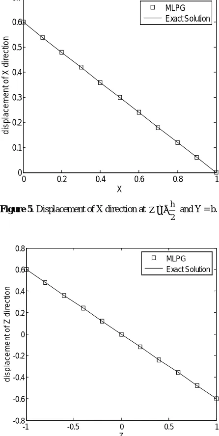
The node distribution with 27 nodes are presented in Figure 4 for the case of L = b = h = 2. The displacement diagrams are shown in Figures 5-7

for the case of .

4 . 2

1 and 6 . 3

1 ,

1 = =

= λ µ

p

As shown in these figures, the MLPG results agree with the values obtained by analytical solution.

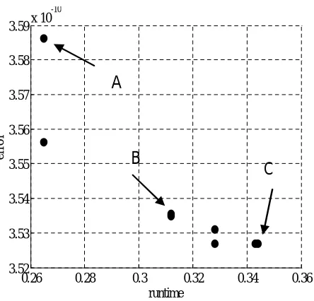
Figure 8 shows the results of multi-objective optimization which all the presented points are non-dominated to each other. Each point in this figure is a representative of a vector of selective parameter. It means that each point on the chart is regarded to the objective functions.

Table 1 shows the different characteristics (error and runtime) of those three selected points.

p

p

p

p

p

Figure 3. Geometric and boundary conditions.

0 0.5

1 1.5

2

0 0.5 1 1.5 2 -1 -0.5 0 0.5 1

Figure 4. The node distribution for example 1.

0 0.2 0.4 0.6 0.8 1

0 0.1 0.2 0.3 0.4 0.5 0.6 0.7

X

d

is

p

la

c

e

m

e

n

t

o

f

X

d

ir

e

c

ti

on

MLPG Exact Solution

Figure 5. Displacement of X direction at

2 h

Z=− and Y = b.

-1 -0.5 0 0.5 1

-0.8 -0.6 -0.4 -0.2 0 0.2 0.4 0.6 0.8

Z

d

is

p

la

c

e

m

e

n

t

o

f

Z

d

ir

e

c

ti

on

MLPG Exact Solution

Figure 6. Displacement of Z direction at

2 L

X= and

2 b

Achieving several answers, all of which are

considered to be optimum, is a unique property of multi-objective optimization. Designer facing several different optimum points from Pareto charts, can easily choose a suitable multisided design point among them.

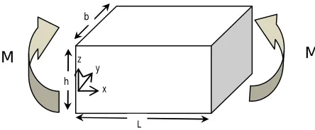
Example 2

The second example is a pure bending of a prismatic bar as illustrated in Figure 9. The node distribution with 225 nodes are presented in Figure 10for the case of L = 4, b = 2 and h = 2.

The exact solutions for this problem are:

R z x u x=−

) 2 (y b R

z

u y=−ν −









_{+ − −}

−

= ) )

2 (

2 2

( 2 2

1 b

y z v x R

u z ₍₃₂₎

y I E

M R =

1

where Iy is the bending stiffness of the plate, as,

12 3

bh y

I =

and

  

   

 

+ + =

strain plane for

stress plane for 2

) 1 (

2 1

E

E E

ν

υ ,

  

   

 

+ =

strain plane for

stress plane for 1

υ

υ υ

υ (33)

The displacements are presented in Figures 11-14 for the plane stress case with E = 1, v = 0.2 and

0 0.2 0.4 0.6 0.8 1

-0.601 -0.6005 -0.6 -0.5995 -0.599

Z

d

is

p

la

c

em

e

n

t

o

f

Y

d

ir

e

c

ti

on

MLPG Exact Solution

Figure 7. Displacement of Y direction at

2 h

Z=− and Y=b.

0.26 0.28 0.3 0.32 0.34 0.36 3.52

3.53 3.54 3.55 3.56 3.57 3.58 3.59x 10

-10

runtime

er

ror

A

B

C

Figure 8. MO Pareto result for example 1.

TABLE 1. Comparison of Points A, B and C of Figure 8.

Point r Error Runtime (s)

A 2.1112615 3.5861834e-010 0.26500000

B 2.7780184 3.5355949e-010 0.31200000

M=1. As shown in these figures, the MLPG results agree surprisingly well with the values obtained by analytical solution.

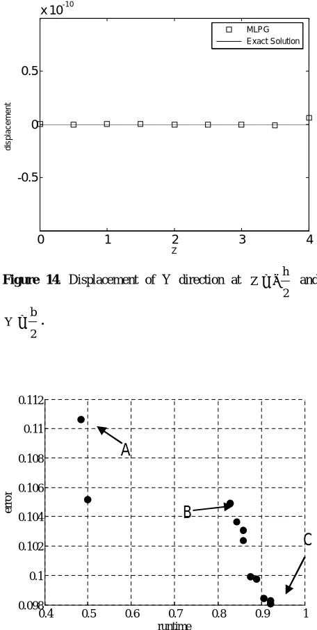
Figure 15 is the chart resulted from multi-objective optimization which all the presented points are non-dominated to each other. As shown in Figure 15, there is a Pareto for the design values regarded to the objective functions

0 1 2 3 4

-0.5 0 0.5 1 1.5 2 2.5 3 3.5

X

d

is

p

la

c

e

m

e

n

t

MLPG Exact Solution

Figure 12. Displacement of X direction at

2 h Z=− and

2 b

Y=

0 1 2 3 4

-7 -6 -5 -4 -3 -2 -1 0

X

d

is

p

la

c

e

m

en

t

MLPG Exact Solution

Figure 13. Displacement of Z direction at

2 h Z=− and

2 b

Y= .

z y

x h

b

L

M M

Figure 9. Geometric and boundary conditions for example 2.

0 ₁

2 _{3 4} 0

0.5 1

1.5 2

-1 0 1

Figure 10. The node distribution for example 2.

-1 -0.5 0 0.5 1

-2 -1.5 -1 -0.5 0 0.5 1 1.5 2

Z

d

is

p

la

c

e

m

en

t

MLPG Exact Solution

Figure 11. Displacement of X direction at

2 L

X= and

2 b

Table 2 also shows the characteristics of the three different design points and their comparative values.

Achieving several answers which all of them are considered optimum is a unique property of multi-objective optimization. Designer in facing to Pareto charts, among several different optimum points can choose a suitable multisided design point easily.

7. CONCLUSIONS

A meshless Local Petrov-Galerkin (MLPG) method is developed for 3D elasto-static problems, based on the local symmetric weak forms. The MLS approximation is used for constructing the trial functions. The penalty approximation is used to impose essential boundary conditions. A simple Heaviside step function is chosen for the test function. Numerical results demonstrate the high accuracy of this method while comparing with the exact solution. As shown, increasing the size of support domain (r) causes the decrease of runtime and the increase of error. The presented points in the Pareto forms resulted from multi-objective optimization. These solutions are non-dominated to each other. Each point in these charts is a representative of a vector of selective parameter. When we choose it for MLPG analysis, the analysis tends to objective functions corresponding to that point of chart. In fact, achieving several answers which all of them are considered optimum is a unique property of multi-objective optimization. Facing to Pareto charts, among several different optimum points, choosing a suitable multisided selective parameter is very easy.

8. REFERENCES

1. Atluri, S.N. and Zhu, T., “A New Meshless Local Petrov-Galerkin (MLPG) Approach in Computational Mechanics”, Comput. Mech., Vol. 24, (1998), 348-372. 2. Lin, H. and Atluri, S.N., “Meshless Local Petrov-Galerkin (MLPG) Method for Convection-Diffusion Problems”,CMES:ComputerModellingin Engineering and Sciences, Vol. 1, No. 2, (2000), 45-60.

TABLE 2. Comparison of Points A, B and C of Figure 15.

Point r Error Runtime (s)

A 2.1314686 0.11063043 0.48400000

B 3.7980912 0.10491221 0.82800000

C 4.8989795 0.098077076 0.92200000

0 1 2 3 4

-0.5 0 0.5

x 10-10

Z

di

s

p

la

c

e

m

en

t

MLPG Exact Solution

Figure 14. Displacement of Y direction at

2 h Z=− and

2 b

Y = .

0.4 0.5 0.6 0.7 0.8 0.9 1

0.098 0.1 0.102 0.104 0.106 0.108 0.11 0.112

runtime

er

ror

A

B

C

3. Wu, Y.L., Liu, G.R. and Gu, Y.T., “Application of Meshless Local Petrov-Galerkin (MLPG) Approach to Simulation of Incompressible Flow”, Numer. Heat Transfer, Part B, Vol. 48, (2005), 459-475.

4. Ching, H.K. and Batra, R.C., “Determination of Crack Tip Fields in Linear Elasto-Statics by the Meshless Local Petrov-Galerkin (MLPG) Method”, CMES: Computer Modelling in Engineering and Sciences, Vol. 2. No. 2, (2001), 273-290.

5. Gu, Y.T. and Liu, G.R., “A Meshless Local Petrov-Galerkin (MLPG) Method for Free and Forced Vibration Analyses for Solids”, Comput. Mech., Vol. 27, (2001), 188-198.

6. Batra, R.C. and Ching, H.K., “Analysis of Elasto-dynamic Deformations near a Crack-Notch Tip by the Meshless Local Petrov-Galerkin (MLPG) Method”,

Comput. Model. Eng. Sci., Vol. 3, No. 6, (2002), 717-730.

7. Gu, Y.T. and Liu, G.R., “A Meshless Local Petrov-Galerkin (MLPG) Formulation for Static and Free Vibration Analysis of Thin Plates”, Comput. Model. Eng. Sci., Vol. 2, No. 4, (2001), 463-476.

8. Long, S.Y. and Atluri, S.N., “A Meshless Local Petrov-Galerkin (MLPG) Method for Solving the Bending Problem of a Thin Plate”, CMES: Computer Modelling in Engineering and Sciences, Vol. 3, No. 1, (2002), 53-63.

9. Han, Z.D. and Atluri, S.N., “Meshless Local Petrov-Galerkin (MLPG) Approaches for Solving 3D Problems in Elasto-Statics”, CMES: Tech Science Press, Vol. 6, No. 2, (2004), 169-188.

10. Han, Z.D. and Atluri S.N., “Truly Meshless Local Petrov-Galerkin (MLPG) Solutions of Traction and Displacement Bies”, CMES: Computer Modeling in Engineering and Sciences,Vol. 4 No. 6 (2003b) 665-678.

11. Han, Z.D. and Atluri, S.N., “A Meshless Local

Petrov-Galerkin (MLPG) Approach for 3 Dimensional Elasto-Dynamics”, CMC: Tech Science Press, Vol. 1, No. 2, (2004), 129-140.

12. Deb, K., Agrawal, S., Pratap, A. and Meyarivan, T., “A Fast and Elitist Multi-objective Genetic Algorithm: NSGA-II”, IEEE Trans Evol Comput, Vol. 6, No. 2, (2002), 182–97.

13. Atashkari, K., Nariman-Zadeh, N., Go¨lcu¨, M., Khalkhali, A. and Jamali, A., “Modelling and Multi-Objective Optimization of a Variable Valve-Timing Spark-Ignition Engine using Polynomial Neural Networks and Evolutionary Algorithms”, Energy Conversion and Management, Vol. 48, (2007), 1029– 1041.

14. Nariman-Zadeh, N., Darvizeh, A. and Ahmad-Zadeh, R., “Hybrid Genetic Design of GMDH-Type Neural Networks using Singular Value Decomposition for Modeling and Prediction of the Explosive Cutting Process”, Proceedings of the IMECHE Part B Journal of Engineering Manufacture, Vol. 217, (2003), 779-790.

15. Atashkari, K., Nariman-Zadeh, N., Pilechi, A., Jamali, A. and Yaob, X., “Thermodynamic Pareto Optimization of Turbojet Engines using Multi-Objective Genetic Algorithms”, International Journal of Thermal Sciences, Vol. 44, (2005), 1061–1071.

16. Nariman-Zadeh, N., Atashkari, K., Jamali, A., Pilechi, A. and Yao, X., “Inverse Modeling of Multi-Objective Thermodynamically Optimized Turbojet Engine using GMDH-Type Neural Networks and Evolutionary Algorithms”, Engineering Optimization, Vol. 37, No. 26, (2005), 437-462.

17. Atashkari, K., Nariman-zadeh, N., Jamali, A. and Pilechi, A., “Thermodynamic Pareto Optimization of Turbojet using Multi-Objective Genetic Algorithm”,