A Particle Swarm Optimization Algorithm for Mixed-Variable Nonlinear Problems

(1)

A PARTICLE SWARM OPTIMIZATION ALGORITHM FOR

MIXED VARIABLE NONLINEAR PROBLEMS

H. Nahvi* and I. Mohagheghian

Department of Mechanical Engineering, Isfahan University of Technology P.O. Box 84156-83111, Isfahan, Iran

*Corresponding Author

(Received: August 26, 2008 – Accepted: July 2, 2009)

Abstract Many engineering design problems involve a combination of both continuous and discrete variables. However, the number of studies scarcely exceeds a few on mixed-variable problems. In this research Particle Swarm Optimization (PSO) algorithm is employed to solve mixed-variable nonlinear problems. PSO is an efficient method of dealing with nonlinear and non-convex optimization problems. In this paper, it will be shown that PSO is one of the best optimization algorithms for solving mixed-variable nonlinear problems. Some changes are performed in the convergence criterion of PSO to reduce computational costs. Two different types of PSO methods are employed in order to find the one which is more suitable for using in this approach. Then, several practical mechanical design problems are solved by this method. Numerical results show noticeable improvements in the results in different aspects.

Keywords Particle Swarm Optimization, Mixed-Variable, Engineering Design

ﻩﺪﻴﻜﭼ

ﺮﻴﻐﺘﻣ ﺯﺍ ﻲﺒﻴﮐﺮﺗ ﻲﺳﺪﻨﻬﻣ ﻲﺣﺍﺮﻃ ﻞﺋﺎﺴﻣ ﺯﺍ ﻱﺭﺎﻴﺴﺑ ﺭﺩ ﻲﻣ ﺭﺎﮐ ﻪﺑ ﻪﺘﺴﺴﮔ ﻭ ﻪﺘﺳﻮﻴﭘ ﻱﺎﻫ

ﺩﻭﺭ . ﻦﻳﺍ ﺎﺑ

ﺖﺳﺍ ﻪﺘﻓﺮﻳﺬﭘ ﻡﺎﺠﻧﺍ ﻞﺋﺎﺴﻣ ﻪﻧﻮﮔ ﻦﻳﺍ ﻱﻭﺭ ﺮﺑ ﻲﻤﮐ ﺕﺎﻌﻟﺎﻄﻣ ﺩﻮﺟﻭ .

ﻲﻌﻤﺟ ﻪﺘﺳﺩ ﺖﮐﺮﺣ ﺵﻭﺭ ﺯﺍ ﻖﻴﻘﺤﺗ ﻦﻳﺍ ﺭﺩ

ﺕﺍﺭﺫ (PSO) ﻪﻨﻴﻬﺑ ﻞﺋﺎﺴﻣ ﻞﺣ ﻱﺍﺮﺑ ﺮﻴﻐﺘﻣ ﻱﺍﺭﺍﺩ ﻲﻄﺧ ﺮﻴﻏ ﻱﺯﺎﺳ

ﺮﺗ ﻱﺎﻫ ﺖﺳﺍ ﻩﺪﺷ ﻩﺩﺎﻔﺘﺳﺍ ﻲﺒﻴﮐ .

PSO ﻲﺷﻭﺭ

ﻲﻣ ﻪﮐ ﺖﺳﺍ ﻪﻨﻴﻬﺑ ﻞﺋﺎﺴﻣ ﻖﻠﻄﻣ ﻪﻨﻴﻬﺑ ﺏﺍﻮﺟ ﻦﺘﻓﺎﻳ ﻱﺍﺮﺑ ﺪﻧﺍﻮﺗ

ﺮﻴﻏ ﻱﺯﺎﺳ ﺮﻴﻏ ﻭ ﻲﻄﺧ

ﻪﺑ ﺏﺪﺤﻣ ﺩﻭﺭ ﺭﺎﮐ . ﻦﻳﺍ ﺭﺩ

ﻲﻣ ﻩﺩﺍﺩ ﻥﺎﺸﻧ ﻪﻟﺎﻘﻣ ﻪﮐ ﺩﻮﺷ

PSO ﺵﻭﺭ ﻦﻳﺮﺘﻬﺑ ﺯﺍ ﻲﮑﻳ ﺮﻴﻐﺘﻣ ﺎﺑ ﻞﺋﺎﺴﻣ ﻞﺣ ﻱﺍﺮﺑ ﺎﻫ

ﺖﺳﺍ ﻲﺒﻴﮐﺮﺗ ﻱﺎﻫ .

ﻲﺗﺍﺮﻴﻴﻐﺗ ﺎﺑ

ﮕﻟﺍ ﻱﺍﺮﺟﺍ ﻥﺎﻣﺯ ﺵﻭﺭ ﻦﻳﺍ ﺭﺩ ﺖﺳﺍ ﻪﺘﻓﺎﻳ ﺶﻫﺎﮐ ﻢﺘﻳﺭﻮ

. ﺵﻭﺭ ﺯﺍ ﻒﻠﺘﺨﻣ ﻉﻮﻧ ﻭﺩ PSO

ﻪﺑ ﺵﻭﺭ ﺯﺍ ﻭ ﻪﺘﻓﺭ ﺭﺎﮐ

ﻖﻴﻗﺩ ﺎﺴﻣ ﺯﺍ ﻱﺩﺍﺪﻌﺗ ﻞﺣ ﺭﺩ ﺮﺗ ﻲﺣﺍﺮﻃ ﻞﺋ

ﺖﺳﺍ ﻩﺪﺷ ﻩﺩﺎﻔﺘﺳﺍ ﻲﺳﺪﻨﻬﻣ .

1. INTRODUCTION

In many engineering optimization problems, the variables cannot accept arbitrary values. That is to say, for practical reasons, some or all of the variables must be selected from a list of integer or discrete values. For example, structural members such as sheets or springs may have to be selected from sections available as standard sizes. Also, the numbers of reinforcement rods in concrete members, bolts in connections, or gear teeth are all integers.

In recent years, considerable interest has been expressed by researchers in the area of mixed-variable optimization. Schmit, et al [1] used dual method for discrete-continuous variables. Sandgrern

[2] and Hajela, et al [3] proposed nonlinear branch and bound algorithms where a solution is first obtained by ignoring the discrete conditions. Typical approach to the solution of optimization problems composed of discrete variables includes sequential linear approach [4], penalty function approach [5], simulated annealing [6] and fuzzy programming [7].

Genetic algorithms (GA) are recently developed optimization techniques and rapidly become popular. Many researchers, including Lin, et al [8], Wu, et al [9], Cheung, et al [10] and Rao, et al [11] considered genetic algorithm to deal with such problems.

(2)

has been proposed by Kennedy, et al [12]. The development of PSO was based on observations of animals, social behavior such as birds flocking and fish schooling. PSO is initialized with a population of random solutions. Each individual is assigned a random velocity according to both its own flying experience and that of its companions. The individual, namely particle, is then flown through hyperspace. PSO has memory so, knowledge of good solution is retained within all particles; whereas for example in GAs, previous knowledge of the problem will be destroyed once the population changes. In PSO there is a mechanism of constructive cooperation and information sharing between particles. Due to its simple concept, easy implementation and quick convergence, PSO has gained much attention and has been successfully applied in a variety of fields.

Several researchers used PSO as a basic algorithm for solving mixed variable problems. Guo, et al [13] presented a hybrid swarm intelligence approach (HSIA) for solving problems containing integer, discrete, zero-one and continuous variables. Zhang, et al [14], and He, et al [15] proposed a co-evolutionary particle swarm optimization approach and a hybrid particle swarm with differential evolution operator, respectively. They also solved some benchmark problems comprised of mixed variable problems.

Elbeltagi, et al [16] compared five evolutionary-based search methods consisting of genetic algorithms, memetic algorithms, particle swarm, ant-colony and shuffled frog leaping. They showed that PSO method performs better than the other algorithms in terms of success rate and solution quality while is preceded by ACO with respect to processing time.

In this paper, two common PSO algorithms are compared and advantages and disadvantages of these algorithms when dealing with mixed discrete nonlinear problems are expressed. Then, by manipulating the convergence criterion, efficiency of the algorithm is improved. Also, two rounding techniques are employed to treat discrete values and the results are compared. Finally, by applying the proposed PSO to numerical examples, it is shown that particle swarm optimization is one of the best methods of solving mixed discrete nonlinear problems.

2. PARTICLE SWARM OPTIMIZATION

The particle swarm optimization (PSO) was inspired by the observations of birds flocking and fish schooling. It differs from other well-known Evolutionary Algorithms (EA) as in EA a population of potential solutions is used to probe the search space; but, no operators, inspired by evolution procedure, are applied on the population to generate a new promising solution. Instead, in PSO, each individual (named particle) of the population (called swarm), adjusts its trajectory towards its own previous best solution (called pbest) and the previous best solution attained by any member of its topological neighborhood. There are different kinds of sharing information between particles. In the global variant of PSO, the whole swarm is considered as the neighborhood. Thus, global sharing of information takes place and the particles benefit from the discoveries and the previous experiences of all other companions during the search for promising regions of the landscape [17]. Alternatively, there are some local variants of PSO wherein particles only make use of their own information and that of the best of their adjacent neighbors.

Each particle in PSO has two main characteristics: its position and its velocity. Assume that the current position and velocity vector of the i-th particle in the d-dimensional search space are denoted as X_i (x_i₁,x_i₂,...,x_id) and V_i(v_i₁,v_i₂,...,v_id), respectively. The best earlier position of the i-th particle is represented as

) pbest ,..., pbest , pbest (

Pbesti i1 i2 id .

There are different kinds of PSO including global vision of PSO with inertia weight (GWPSO), local vision of PSO with inertia weight (LWPSO), global vision of PSO with constriction factor (GCPSO), and local vision of PSO with constriction factor (LCPSO) [18].

In GWPSO, which is very popular among researchers, there are two methods for updating position and velocity of each particle. The best position of entire group at k-th iteration is used in the first method while in the second method; the best position of entire group up to the current search is employed.

In the first method, the position k id

(3)

updated as follows: 1 k id v k id x 1 k id

x     (1)

) k id x gbest ( 2 r 2 c ) k id x k id pbest ( 1 r 1 c k id wv

1 k id v

 

 

(2)

In Equation 2 w is the inertia weight, c1 and c2

are positive constants called cognitive and social parameters, respectively, and r1 and r2 are random

numbers selected in the interval [0 1]. The constants c1 and c2 represent the weighting of the

stochastic acceleration terms that pull each particle towards pbest and gbest positions and usually are setc1c22.

In the second method gbest is replaced

by k

gbest . As will be shown later, in the numerical examples of mixed-variables or in the problems that only have discrete variables, usage of gbestk is more suitable compared to the use ofgbest. In other words, the success rate of k

gbest is higher than that of gbest. The reason is firstly due to the fast convergence of gbestand secondly, the inability of particles to escape from local minima in gbest method. In other words, since the discrete variables are rapidly converged the continuous variables will be obliged to search in a limited specific area which might not be the optimum area. The role that inertia weight w plays in the convergence behavior of PSO is very important. The inertia weight is employed to control the effect of the previous velocities on the current velocity. This way, the parameter w makes a compromise between global and local exploration abilities of the swarm. In PSO, when the search continues, the inertia term decreases linearly as:

k ) max k

min w max w ( max w w

 

 (3)

where wmax and wmin are the maximum and

minimum values of the inertia term, respectively, and kmax is the maximum number of iterations. In

this paper, these parameters are assumed to be:

1 max

w  , w_min 0 (4)

Sometimes as particle oscillations become wider, the system will gain tendency to explode [12]. The usual means of preventing explosion is simply to define a parameter vmax and curb the velocity of

every individual i from exceeding that velocity on each dimension d. In the case that velocity violates, it will be modified as follows:

If v_idv_max then v_idv_max

If v_idv_max then v_idv_max (5) The effect of this is to allow particles to oscillate

within the bounds [12].

2.1. Mathematical Formulation of Constraint

Problems

Problem definition:

Minimize f(x) Subject to

U i x i x L i

x   i1,2,...,n (6)

0 ) x ( h

g  h1,2,...,m (7)

where n is the number of continuous variables, L i x

and xUi are the lower and upper bounds of

continuous variables, respectively, gh(x) are applied constraints and m is the number of constraints.

Penalty function is defined as:

 

 

 m 2n

1 h

)} x ( h g , 0 max{ r

) x ( f ) x (

F (8)

where r is the penalty parameter, m + 2n is the number of all inequality constraints including

) x (

g_h and two supplemental constraints, related to the upper and lower bounds of each continuous variable.

(4)

the number of discrete variables in the problem is s: i

D i n

x _ 

} f , i d ,..., 2 , i d , 1 , i d { i

D  i1,2,...,s (9)

At first these variables are treated as continuous and similar to above, the following supplemental constraints are applied for the upper and lower bounds

f , i d i n x 1 , i

d  _  i1,2,...,s (10) The new objective function incorporates the

behavior constraints as:  

 

 m 2n 2s

1 h

)} x ( h g , 0 max{ r

) x ( f ) x (

F (11)

At any iteration, after finding the new position of particles(xk1), appropriate variables can be made discrete using two methods. The first method is to find the nearest discrete value to the current continuous variable as follows:

q , i d i n x q , i d i n x f , i d i n x

,..., 2 , i d i n x , 1 , i d i n x min

            

 _

 



(12)

The second method is to check the upper and lower discrete values of the current continuous variable and determine which one is the best. It is obvious that second method imposes additional fitness calls to the solution and accordingly increases computational costs. However, when the range of discrete variables is vast, usage of second method leads more accurate results and better convergence [19].

Using these two methods, at any iteration, all of discrete variables that are treated as continuous become discrete. These methods are very simple and efficient and do not have the complexities of the penalty approach. They also surmount shortcomings existing in the methods that adopt discrete values near the optimal solution or use discrete values obtained by rounding off.

2.3. Convergence Criterion

In practice, after some iterations all of the particles converge to a

specific part of problem’s space and with subsequent iterations, particles only oscillate in that region. These oscillations only increase the precision of results. Most of the times such high precision is unnecessary so, a convergence criterion is introduced based on the required accuracy. When the results attained such accuracy, iterations will be terminated and do not need to reachkmax. This can decrease the number of fitness

calls and as a result reduce the computational costs. This reduction is more significant in the cases of mixed or discrete variable problems. The convergence criterion is determined as:

) ij V min( min

v  i1,2....,c j1,2,....,d

Terminate if min

v < e (13)

where c and d are the number of variables and particles, respectively, and e is the required accuracy.

2.4. Optimization Algorithm of Mixed

Discrete Variables Problems

The algorithm of the proposed method is as follows:

1. The number of particles and maximum number of iterations are determined. The iteration number k is set to k = 1.

2. The position and velocity for every particle are set at random.

3. The due variables are made discrete. 4. The values of pbestk, gbestk and gbest

are determined.

5. The value of inertia weight is calculated. 6. The position and velocity of every

particle are updated by k

pbest and

k

gbest .

7. If the velocity of particles violate vmax

and vmax they are modified.

8. If the minimum value of the particle’s absolute velocity is lower than what was chosen; jump to 11.

9. k = k + 1

10. The number of iterations is checked. If

max

k

(5)

3. NUMERICAL EXAMPLES

To demonstrate the effectiveness of the proposed approach, several applications of optimum design, each corresponds to a particular class, are considered. In the welded beam design the entire variables are continuous while, in the speed reducer design, all of the variables are discrete. In the pressure vessel problem variables are combination of discrete and continuous. In the coil compression spring design problem continuous, discrete and integer variable are exist.

3.1. Example 1. Welded Beam Design

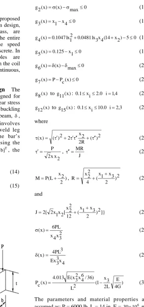
The welded beam shown in Figure 1 is designed for minimum cost subject to constraint on shear stress in weld, , bending stress in beam,, buckling load on the bar, Pc, end deflection of the beam, ,

and side constraints. This problem involves four continuous variables; the fillet weld leg size, h, the fillet weld length, l, the bar’s width, t, and the bar’s thickness, b. Using the design vector X[x1,x2,x3,x4]T [h,l,t,b]T, the

objective function and constraints are ) 2 x 14 ( 4 x 3 x 0481 . 0 2 x 2 1 x 10471 . 1 ) x (

f    (14)

0 max ) x ( ) x ( 1

g    (15)

0 max ) x ( ) x ( 2

g    (16)

0 4 x 1 x ) x ( 3

g    (17)

0 5 ) 2 x 14 ( 4 x 3 x 04811 . 0 2 1 x 10471 . 0 ) x ( 4

g      (18)

0 1 x 125 . 0 ) x ( 5

g    (19)

0 max ) x ( ) x ( 6

g    (20)

0 ) x ( c P P ) x ( 7

g    (21)

) x ( 8

g to g₁₁(x): 0.1x_i2.0 i1,4 (22)

) x ( 12

g to g₁₅(x): 0.1x_i10.0 i2,3 (23) where 2 ) ( R 2 2 x 2 2 ) ( ) x (      

 (24)

2 x x 2 P   , J MR 

  (25)

) 2 2 x L ( P

M  , )2

2 3 x 1 x ( 4 2 2 x

R   (26)

and ]} 2 ) 2 3 x 1 x ( 12 2 2 x [ 2 x 1 x 2 { 2

J   (27)

2 3 x 4 x PL 6 ) x ( 

 (28)

4 x 3 3 Ex 3 PL 4 ) x ( 

 (29)

) G 4 E L 2 3 x 1 ( 2 L ) 36 / 6 4 x 2 3 x ( E 013 . 4 ) x ( c

P   (30)

The parameters and material properties are assumed as: P = 6000 lb, L = 14 in, E = 30106 psi, G = _12₁₀6_psi, ₁₃₆₀₀

max 

 psi, _max 30000 psi and _max 0.25 in.

(6)

TABLE 1. Comparison of the Best Solution for Example 1 Found by Different Methods.

Ragsedell Deb Coello He Research

) h (

x₁ _0.245500 _0.248900 _0.208800 _0.202369 _0.20572276 )

(

x₂ l _6.196000 _6.173000 _3.420500 _3.544214 _3.4707008

) t (

x₃ _8.273000 _8.178900 _8.997500 _9.048210 _9.03681306 )

b (

x₄ _0.245500 _0.253300 _0.210000 _0.205723 _0.20572878 )

x (

g₁ _-5743.8265 _-5758.6037 _-0.337812 _-12.839796 _-0.4287188 )

x (

g₂ _-4.715097 _-255.5769 _-353.902604 _-1.247467 _-1.13037 )

x (

g₃ _0.000000 _-0.004400 _-0.001200 _-0.001498 _-0.0000006 )

x (

g₄ _-3.020289 _-2.982866 _-3.411865 _-3.429347 _-3.4329389 )

x (

g₅ _-0.120500 _-0.123900 _-0.083800 _-0.079381 _-0.0807227 )

x (

g₆ _-0.234208 _-0.234160 _-0.235649 _-0.235536 _-0.2355411 )

x (

g₇ _-3604.275 _-4465.2709 _-363.23238 _-11.681355 _-0.0088613 )

x (

f _2.385937 _2.433116 _1.748309 _1.728024 _1.7248965

TABLE 2. Statistical Results of Different Methods for Example 1.

Ragsdell [22] 2.385937 N/A N/A N/A

Deb [23] 2.433116 N/A N/A N/A

Coello [24] 1.748309 1.771973 1.785835 0.011220

He [15] 1.728024 1.748831 1.782143 0.012926

This Research 1.724897 1.730813 1.767000 0.010281 In this example, the number of particles,

maximum iterations number and convergence criterion value are assumed to be 30, 1000 and 10

-6

, respectively. The results are obtained through 30 independent runs. Table 1 lists the welded beam design results obtained by different researchers. As can be seen, the objective function value gained in this research is the best compare to the results of other researches. The statistical results are shown in Table 2. It is evident that not only the best feasible solution obtained in this paper is the best among other researches also, the average searching quality and the worst solution is better than those of other techniques. The standard deviation of the results of this research is very small.

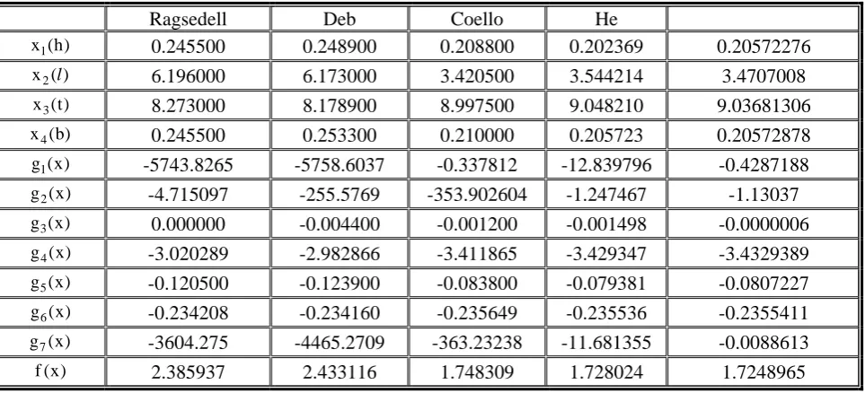
3.2. Example 2. Pressure Vessel Design

Optimum design of a pressure vessel is one of the most famous benchmarks for mixed discrete nonlinear programming (MDNLP) problems and several studies of it are available. The pressure vessel is an air storage tank (as shown in Figure 2) with a working pressure of 3000 psi and a minimum volume of 750 ft . The cylindrical pressure vessel 3 is capped at both ends by hemispherical heads. Using rolled steel plate, the shell is to be made in two halves that are joined by two longitudinal welds to form a cylinder. Each head is forged and then welded to the shell. Four design variables are

considered as s h T

T 4 3 2

1,x ,x ,x ] [T,T ,R,L] x

[

X 

(7)

of the head, Th, the inner radius, R and length of

the cylindrical section, L. Among the variables R and L are continuous while, Ts and Th are discrete

and required to be a standard size (multiple of 0.0625 in). This problem is formulated according to the ASME boiler and pressure vessel code. The objective function is to minimize the total cost of material used, forming, and welding of the pressure vessel. The problem may be mathematically stated as:

Minimize

3 x 2 1 x 84 . 19 4 x 2 1 x 1661 . 3

2 3 x 2 x 7781 . 1 4 x 3 x 1 x 6224 . 0 ) x ( f



 



(31)

Subject to the following behavior and side constraints

0 1 1 x

3 x 0193 . 0 ) x ( 1

g    (32)

0 1 2 x

3 x 00954 . 0 ) x ( 2

g    (33)

0 1 4

x 2 3 x

3 3 x 3 4 1728 750 ) x ( 3

g  



  

 (34)

0 1 240

4 x ) x ( 4

g    (35)

25 . 1 i x 0625 .

0   i1,2

k 0625 . 0 i

x  k1,2...,20 (36)

150 3 x

25  (37)

240 4 x

25  (38)

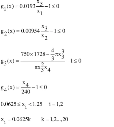
Different techniques are employed by researchers for solving this problem. Table 3 indicates a number of results obtained by researchers using particle swarm optimization as the basic solution algorithm while Table 4 shows the results gained by using other methods.

The results of this research, shown in Table 3, are obtained by considering 50, 500, 106 as the number of particles, maximum iterations number and convergence criterion, respectively.

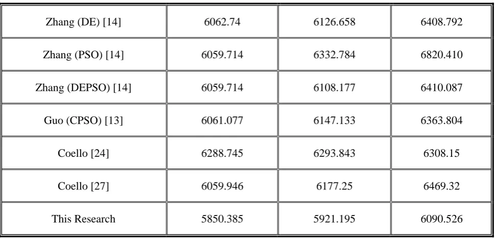
As shown in Table 4, the best objective function value obtained by methods excluding particle swarm is 5850.77, credited to adaptive range genetic algorithm (ARGA) [20]. The presented approach found a slightly better optimal solution (5850.385) of the pressure vessel problem. Additionally, it is the best solution among the methods that implemented PSO. On the other hand, the average of function calls in the present solution is 22200 while this value is 30000, and 49000 according to binary method [21] and DEPSO [14], respectively. The number of function calls in CPSO [13] is 200000 and in GA-base is 900000 [9]. The number of function calls is a criterion of measuring the computational cost. Since this value is not reported by all researchers the computational cost can not be properly compared in all the researches.

The statistical results of different methods are shown in Table 5. Significant improvement can be seen in three fields of best solution, worst solution and the average search quality as a result of the work done in this study. As discussed in the previous sections, when the problem consists of a combination of both discrete and continuous variables the usage of k

gbest is more efficient than use of gbest. This fact can be concluded from Table 6. It is evident from the table that by increasing the number of particles or the maximum iterations value, the improvement will be more significant in attempts that use gbestk.

(8)

TABLE 3. Results of Example 2 using Particle Swarm Optimization as the Basic Solution Technique.

This Research Zhang

Kitayama He

He Guo

38.860 42.1

36.684 42.1

42.091 58.29

R

221.365 176.64

224.096 176.64

176.747 43.7

L

0.75 0.8125

0.8125 1.125

s T

0.375 0.4375

0.4375 0.625

h T

0 0

-0.004 0

0 0

1 g

-0.0014 -0.08

-0.016 -0.08

-0.036 -0.0689

2 g

0 -0.26

-0.066 --0.26

0.036 -69.24

3 g

-0.0776 0

0.00 0

-63.26 -196.3

4 g

5850.385 6059.7

5875.254 6059.7

6061.077 7197.9

Cost

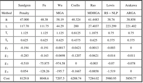
TABLE 4. Results of Example 2 Obtained by Different Methods Excluding Particle Swarm Optimization Technique.

Arakawa Lewis]

Rao]

Coello]

Wu Fu

Sandgren

ARGA RS + NLP

MDHGA MGA

Penalty Method

38.858 38.76

61.4483 40.324

58.19 48.38

47.000

R

221.402 223.299

27.4037 200

44.29 111.75

117.70

L

0.75 0.75

1.1875 0.8125

1.125 1.125

1.125

s T

0.375 0.375

0.625 0.4375

0.625 0.625

0.625

h T

0 -0.003

-0.0013 -0.0421

-0.0017 -0.191

-0.194 1

g

-0.011 -0.014

-0.0621 -0.1207

-0.0698 -0.163

-0.283 2

g

-0.078 -0.07

-0.003 0

-974.58 -75.875

-0.510 3

g

0 -1.519

-0.8858 -0.1667

-195.7 -128.26

0.054 4

g

5850.77 5980.95

7284.02 6288.74

7207.5 8048.6

(9)

TABLE 5. Statistical Results of Different Methods for Example 2.

6408.792 6126.658

6062.74 Zhang (DE) [14]

6820.410 6332.784

6059.714 Zhang (PSO) [14]

6410.087 6108.177

6059.714 Zhang (DEPSO) [14]

6363.804 6147.133

6061.077 Guo (CPSO) [13]

6308.15 6293.843

6288.745 Coello [24]

6469.32 6177.25

6059.946 Coello [27]

6090.526 5921.195

5850.385 This Research

TABLE 6. Comparison of gbestand gbestk for Different Solutions of Example 2.

5/30 6090.6

6009.7 5850.38

2000 10

k

gbest

7/30 6163.9

6002.0 5850.38

2000 15

k gbest

9/30 6090.7

5991.7 5850.38

4000 10

k gbest

16/30 6090.5

5921.95 5850.38

500 50

k

gbest

4/30 6424.1

6146.6 5850.38

2000 10

gbest

4/30 6726.5

6125.3 5850.38

2000 15

gbest

7/30 6820.4

6082.1 5850.38

4000 10

gbest

5/30 6411.0

6083.6 5850.38

500 50

(10)

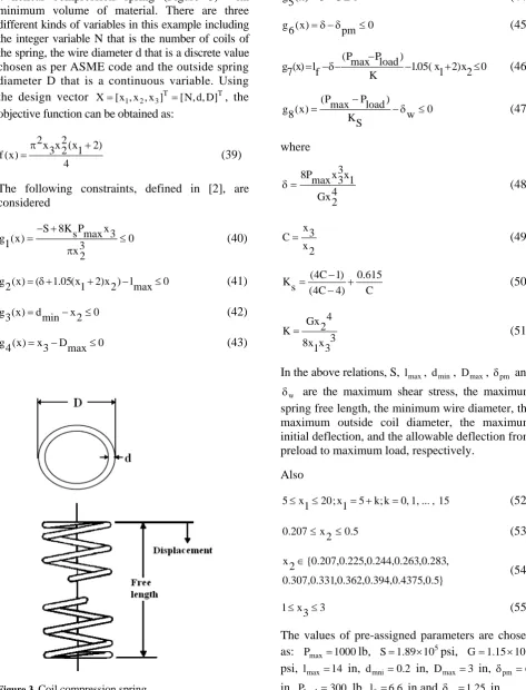
a helical compression spring (Figure 3) with minimum volume of material. There are three different kinds of variables in this example including the integer variable N that is the number of coils of the spring, the wire diameter d that is a discrete value chosen as per ASME code and the outside spring diameter D that is a continuous variable. Using the design vector X[x1,x2,x3]T [N,d,D]T, the

objective function can be obtained as:

4 ) 2 1 x ( 2 2 x 3 x 2 ) x (

f   (39) The following constraints, defined in [2], are considered 0 3 2 x 3 x max P s K 8 S ) x ( 1 g    

 (40)

0 max l ) 2 x ) 2 1 x ( 05 . 1 ( ) x ( 2

g      (41)

0 2 x min d ) x ( 3

g    (42)

0 max D 3 x ) x ( 4

g    (43)

0 C 3 ) x ( 5

g    (44)

0 pm ) x ( 6

g   (45)

0 2 x ) 2 1 x ( 05 . 1 K ) load P max P ( f l ) x ( 7

g   

   

 (46)

0 w S K ) load P max P ( ) x ( 8

g     (47)

where 4 2 Gx 1 x 3 3 x max P 8 

 (48)

2 x

3 x

C (49)

C 615 . 0 ) 4 C 4 ( ) 1 C 4 ( s K   

 (50)

3 3 x 1 x 8 4 2 Gx

K (51)

In the above relations, S, lmax, dmin, Dmax, pm and w

 are the maximum shear stress, the maximum spring free length, the minimum wire diameter, the maximum outside coil diameter, the maximum initial deflection, and the allowable deflection from preload to maximum load, respectively.

Also 15 , ... , 1 , 0 k ; k 5 1 x ; 20 1 x

5     (52)

5 . 0 2 x 207 .

0   (53)

} 5 . 0 , 4375 . 0 , 394 . 0 , 362 . 0 , 331 . 0 , 307 . 0 , 283 . 0 , 263 . 0 , 244 . 0 , 225 . 0 , 207 . 0 { 2 x  (54) 3 3 x

1  (55)

The values of pre-assigned parameters are chosen as: P_max1000lb, S1.89105psi, G1.15107

psi, lmax14 in, dmni 0.2 in, Dmax3 in, pm 6

(11)

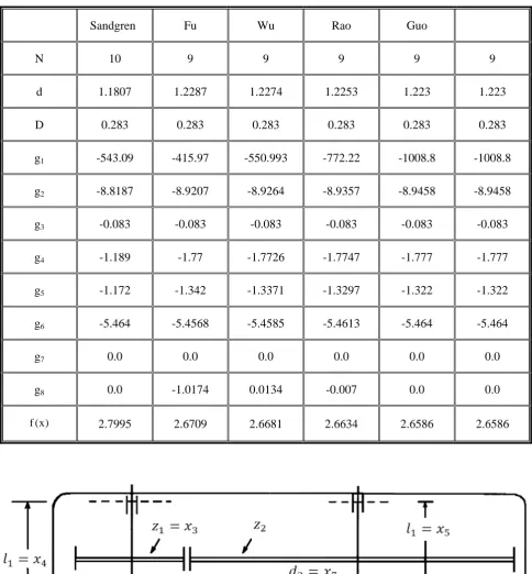
In this example, the number of particles, maximumiterationsvalue and convergence criterion are assumed to be 10, 1000, 10-6, respectively. The optimum results obtained by the present approach are compared with the results reported in the literature, presented in Table 7. Results of this research is similar to those achieved by Guo, et al [13] using HSIA and is the best result compare to the other researches. Among 30 independent runs, 24 runs find the global optimum (2.6586). The average of function calls in this problem is 7738.

3.4. Example 4. Speed Reducer (Gear Train)

In this example optimum design of a the speed reducer, shown in Figure 4, is considered. Design variables are face width, b, the teeth module, m, the number of pinion teeth, n, length of shaft 1 between bearings, l1, length of the shaft 2

between bearings, l2, diameter of shaft 1, d1 and

diameter of shaft 2, d2. The design vector is defined

as: T

2 1 2 1 T 7 6 5 4 3 2

1,x ,x ,x ,x ,x ,x ] [b,m,n,l,l ,d,d ] x

[

X 

where x3 is an integer variable, x1, x2, x4and x5

are defined as integer multiples of 0.1, x6 and x7

are defined as integer multiples of 0.01. The objective is to minimize the total weight of speed reducer. The constraints include limitation on the bending stress and surface stress of the gear teeth, and transverse deflection of the shafts 1 and 2 [11]. The mathematical formulation of the problem is: Minimize ) 2 7 x 5 x 2 6 x 4 x ( 7854 . 0 ) 3 7 x 3 6 x ( 477 . 7 ) 2 7 x 2 6 x ( 1 x 508 . 1 ) 0934 . 43 3 x 9334 . 14 2 3 x 3333 . 3 ( 2 2 x 1 x 7854 . 0 ) x ( f           (56) Subject to the following constraints

0 1 3 x 2 2 x 1 x 27 ) x ( 1

g    (57)

0 1 2 3 x 2 2 x 1 x 5 . 397 ) x ( 2

g    (58)

0 1 4 6 x 3 x 2 x 3 4 x 93 . 1 ) x ( 3

g    (59)

0 1 4 7 x 3 x 2 x 3 5 x 93 . 1 ) x ( 4

g    (60)

0 1100 } 3 6 x 1 . 0 5 . 0 ] 6 10 ) 9 . 16 ( 2 ) 3 x 2 x 4 x 745 [( { ) x ( 5 g     (61) 0 850 } 3 7 x 1 . 0 5 . 0 ] 6 10 ) 5 . 157 ( 2 ) 3 x 2 x 5 x 745 ( [ { ) x ( 6 g     (62) 0 40 3 x 2 x ) x ( 7

g    (63)

0 2 x 1 x 5 ) x ( 8

g    (64)

0 12 2 x 1 x ) x ( 9

g    (65)

0 1 4 x ) 9 . 1 6 x 5 . 1 ( ) x ( 10

g     (66)

0 1 5 x ) 9 . 1 7 x 1 . 1 ( ) x ( 11

g     (67)

6 . 3 1 x 6 .

2   (68)

8 . 0 2 x 7 .

0   (69)

28 3 x

17  (70)

3 . 8 4 x 3 .

7   (71)

3 . 8 5 x 3 .

7   (72)

9 . 3 6 x 9 .

2   (73)

5 . 5 7 x 0 .

5   (74)

(12)

TABLE 7. Best Results Obtained by Other Researches for Example 3.

Research Guo

Rao Wu

Fu Sandgren]

9 9

9 10

N

1.223 1.223

1.2253 1.2274

1.2287 1.1807

d

0.283 0.283

D

-1008.8 -1008.8

-772.22 -550.993

-415.97 -543.09

g1

-8.9458 -8.9458

-8.9357 -8.9264

-8.9207 -8.8187

g2

-0.083 -0.083

g3

-1.777 -1.777

-1.7747 -1.7726

-1.77 -1.189

g4

-1.322 -1.322

-1.3297 -1.3371

-1.342 -1.172

g5

-5.464 -5.464

-5.4613 -5.4585

-5.4568 -5.464

g6

0.0 0.0

g7

0.0 0.0

-0.007 0.0134

-1.0174 0.0

g8

2.6586 2.6586

2.6634 2.6681

2.6709 2.7995

) x ( f

(13)

identical to the solution reported by Rao, et al [11], obtained by MDHGA method. The constraints values g1(x) to g11(x) are -0.0739, -0.198, -0.5050,

-0.9017, -9.5826, -1.5978, -28.1, 0, -7, -0.0493, -0.0104, respectively. This implies that the optimum solution is in the feasible region.

4. CONCLUSION

In this paper the particle swarm optimization algorithm is employed to solve mixed-variable nonlinear problems. Two common PSO algorithms were compared and results of engineering design problems show that for mixed-discrete problems gbestk has better performance. Also some changes are performed in the convergence criterion. Simulation results for four constrained engineering design problems are compared with the previously reported results. Noticeable improvements are observed in the results.

5. REFERENCES

1. Schmit, L.A. and Fleury, C., “Discrete-Continuous

Variable Structural Synthesis Using Dual Method”,

AIAA Journal, Vol. 18, (1980), 1515-1524.

2. Sandgren, E., “Nonlinear Integer and Discrete

Programming in Mechanical Design Optimization”,

ASME, Journal of Mechanical Design, Vol. 112,

(1990), 223-229.

3. Hajela, P. and Shih, C., “Multiobjective Optimum

Design in Mixed-Integer and Discrete Design Variable Problems”, AIAA Journal, Vol. 28, (1989), 670-675.

4. Loh, H.T. and Papalambros, P.Y., “A Sequential

Linearization Approach for Solving Mixed-Discrete

Nonlinear Design Optimization Problems” ASME,

Journal of Mechanical Design, Vol. 113, (1991a),

325-334.

5. Fu, J.F., Fenton, R.G. and Cleghorn, W.L., “A Mixed

Integer-Discrete-Continuous Programming Method and its Application to Engineering Design Optimization”,

Eng. Optimization, Vol. 17, (1991), 263-280.

6. Zhang, C. and Wang, H.P., “Mixed-Discrete Nonlinear

Optimization with Simulated Annealing”, Eng.

Optimization, Vol. 21, (1993), 277-291.

7. Shih, C.J. and Lai, T.K., “Mixed-Discrete Fuzzy

Programming for Nonlinear Engineering Optimization”,

8. Lin, C.Y. and Hajela, P., “Genetic Algorithms in

Optimization Problems with Discrete and Integer Design Variables”, Eng. Optimization, Vol. 19, (1992),

309-327.

9. Wu, S.J. and Chow, P.T., “Genetic Algorithms for

Nonlinear Mixed Discrete-Integer Optimization Problems via Meta-Genetic Parameter Optimization”,

10. Cheung, B.K.-S., Langevin, A. and Delmaire, H.,

“Coupling Genetic Algorithm with s Grid Search Method to Solve Mixed Integer Nonlinear Programming Problems”, Comput. Math. Appl., Vol. 34, (1997), 13-23.

11. Rao, S.S. and Xiang, Y., “A Hybrid Genetic Algorithm

for Mixed-Discrete Design Optimization”, ASME,

Journal of Mechanical Design, Vol. 127, (1992),

1100-1112.

12. Kennedy, J., Eberhart, R.C. and Shi, Y. (Eds.), “Swarm Intelligence”, Morgan Kaufmann, San Francisco, U.S.A., (2001).

13. Guo, X., Hu, J.-X., Ye, B. and Cao, Y.-J., “Swarm

Intelligence for Mixed-Variable Design Optimization”,

J. Zhejiang Univ. SCI., Vol. 5, (2004), 851-860.

14. Zhang, W.J. and Xie, X.F., “DEPSO: Hybrid Particle

Swarm with Differential Evolution Operator”, IEEE

Int. Conference on Systems and Cybernetics, (2003),

3816-3821.

15. He, Q. and Wang, L., “An Effective Co-Evolutionary

Particle Swarm Optimization for Constrained Engineering

Design Problems”, Engineering Applications of

Artificial Intelligence, Vol. 20, (2007), 89-99.

16. Elbeltagi, E., Hegazy, T. and Grierson, D., “Comparison Among Five Evolutionary-Based Optimization Algorithms”, Advanced Engineering Informatics, Vol. 19, (2005), 43-53.

17. Laskari, E.C., Parsopoulos, K.C. and Vrahatis, M.N.,

“Particle Swarm Optimization for Integer Programming”,

Proceedings IEEE Congress on Evolutionary

Computation, Hawaii, U.S.A., (2002), 1576-1581.

18. Yu, B., Yuan, X. and Wang, J., “Short-Term

Hydro-Thermal Scheduling using Particle Swarm Optimization

Method”, Energy Conversion and Management, Vol.

48, (2007), 1902-1908.

19. Kitayama, S. and Yasuda, K., “A Method for Mixed

Integer Programming by Particle Swarm Optimization”,

Electrical Engineering in Japan, Vol. 157, No. 2.

(2006), 40-49.

20. Arakawa, M., Ishikawa, H. and Miyashita, T., “Genetic Range Genetic Algorithm to Obtain Quasi-Optimum Solutions Proc ASME/DETC/DAC”, Paper No. 48800, in CDROM, (2003).

21. Kitayama, S., Arakawa, M. and Yamazaki, K., “Penalty

Function Approach for the Mixed Discrete Problems by Particle Swarm Optimization”, Struc. Multidisciplinary

Optimization, Vol. 32, (2006), 191-202.

22. Ragsdell, K.M. and Phillips, D.T., “Optimal Design of a Class of Welded Structures using Geometric

Programming”, ASME, Journal of Engineering for

Industry, Vol. 98, No. 3, (1976), 1021-1025.

23. Deb, K., “Optimal Design of a Welded Beam via

Genetic Algorithms”, AIAA Journal, Vol. 29, No. 11, (1991), 2013-2015.

24. Coello, C.A.C., “Use of a Self-Adaptive Penalty

Approach for Engineering Optimization Problems”,

(14)

25. He, S., Prempian, E. and Wu, Q.H., “An Improved Particle Swarm Optimizer for Mechanical Design Optimization Problems”, Eng. Optimization, Vol. 36, No. 5, (2004), 585-605.

26. Lewis, K. and Mistree, F., “Foraging-Directed Adaptive Linear Programming: An Algorithm for Solving Nonlinear Mixed Discrete/Continuous Design Problems”

Proc. ASME/DETC/DAC, Paper No. 1601, in CDROM, (1996).

27. Coello, C.A.C., “Theoretical and Numerical Constraint Handling Techniques used with Evolutionary Algorithms: A Survey of the State of the Art”, Computer Methods

in Applied Mechanics and Engineering, Vol. 191, No.