Two and Three-Dimensional Seepage Analysis of Earth Dams Considering Horizontal Filter Blanket Effects (RESEARCH NOTE)

International Journal of Engineering Vol. 18, No. 2, May 2005 -187

RESEARCH NOTE

TWO AND THREE-DIMENSIONAL SEEPAGE ANALYSIS OF EARTH

DAMS CONSIDERING HORIZONTAL FILTER BLANKET EFFECTS

S.M. Marandi, P. Safapour, R.Movahed Asl and M.H. Bagheripour Department of Civil Engineering, Shahid Bahonar University, Kerman, Iran

[email protected] , [email protected] , [email protected] , [email protected]

(Received: Jan. 17, 2004– Accepted in Revised Form: Aug. 5, 2005)

Abstract The amount of seepage which crosses the body of earth dams is considered by several scientists. Despite of these researches and studies that carried out by technical experts and scientists, still the effect of positioning horizontal filter blankets on two and three dimensional seepage analysis are not analyzed in full details. In this paper, the effects of variation in the location of the horizontal filter blankets are studied. The results showed that the amount of flux is greatly influenced by the place of the horizontal filter blanket and it has more effect on flux in three-dimensional models than that of two-dimensional ones.

Keywords Measurement, Mobile robot, Test, Experimental Analysis.

ﺪﻴﻜﭼ ﻩ

ﺖـﺳاهدﻮـﺑﻦﻴـﻘﻘﺤﻣزايرﺎﻴﺴـﺑﻪـﺟﻮﺗدرﻮـﻣﻲﻛﺎﺧيﺎﻫﺪﺳﻪﻧﺪﺑزايرﻮﺒﻋﺖﺸﻧناﺰﻴﻣ

. وتﺎـﻌﻟﺎﻄﻣﻢﻏﺮـﻴﻠﻋ

يﺪـﻌﺑﻪـﺳويﺪـﻌﺑودﺖﺸـﻧيورﺮﺑﻲﻘﻓاﺶﻜﻫزﺖﻴﻌﻗﻮﻣتاﺮﻴﺛﺎﺗزﻮﻨﻫ،ﻦﻴﻘﻘﺤﻣونﺎﺳﺎﻨﺷرﺎﻛﻂﺳﻮﺗهدﺮﺘﺴﮔتﺎﻘﻴﻘﺤﺗ

ﺖﺳاﻪﺘﻓﺮﮕﻧراﺮﻗﻞﻣﺎﻛﻞﻴﻠﺤﺗوﻪﻳﺰﺠﺗدرﻮﻣ

.

ﺮﺛاﻪﻟﺎﻘﻣﻦﻳارد

راﺮـﻗﻪـﻌﻟﺎﻄﻣدرﻮـﻣﻲـﻘﻓاﺶﻜﻫزﻲﻧﺎﻜﻣﺖﻴﻌﻗﻮﻣردﺮﻴﻴﻐﺗتا

ﺖﺳاﻪﺘﻓﺮﮔ

. ﻲﻛﺎـﺧيﺎﻫﺪﺳﻪﻧﺪﺑردﺖﺸﻧﺰﻴﻟﺎﻧآيورﺮﺑﻲﻬﺟﻮﺗﻞﺑﺎﻗﺮﺛاﻲﻘﻓاﺶﻜﻫزﻲﻧﺎﻜﻣﺖﻴﻌﻗﻮﻣﻪﻛﺪﻫﺪﻴﻣنﺎﺸﻧﺞﻳﺎﺘﻧ

دراد

.

ﺖﺳايﺪﻌﺑوديﺎﻬﻟﺪﻣزاﺮﺗراﺬﮔﺮﻴﺛﺎﺗيﺪﻌﺑﻪﺳيﺎﻬﻟﺪﻣردﻲﻘﻓاﺶﻜﻫزنﺎﻜﻣﻦﻴﻨﭽﻤﻫ

.

1. INTRODUCTION

One of the main criteria for designing an earth dam is the amount of seeping water through its body. Hence an accurate estimate of the amount of seeping water is very important from the economical and technical view points.

Flow of water in the body of an earth dam causes seepage forces, pore water pressure and hydraulic gradients. If these forces exceed allowable ranges, they may develop some problems such as instability of slopes, piping, etc, which may ultimately lead to failure of the dam.

Thus, seepage analysis in the design of an earth dam is also important from the safety purpose. Therefore, an accurate analysis of seepage is

crucial. Because of some difficulties in three-dimensional seepage analysis, for practical purposes, a two-dimensional analysis is usually carried out in a typical cross section of dam. However, this simplification can mislead especially when dam has a horizontal filter blanket in its down stream side.

estimate of flux but they all failed in a correct manner.

In this paper, three dimensional seepage analyses have been performed for homogenous earth dams with horizontal filter blanket. Also two-dimensional seepage analysis has been carried out for these dams. The results have been compared with Kozeny’s solution and a new model is introduced which can estimate the amount of flux.

2. THEORY

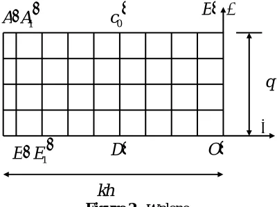
An earth dam section abcd is shown in figure (1) with horizontal filter blanket along the base, which drains the seepage water. If this blanket does not exist, the free surface emerges at the dawn stream slope. Because the horizontal filter blanket is in contact with atmosphere pressure, it directs all flow lines within the body of earth dam away from the dawn stream surface, increasing its stability and preventing erosion along the dawn stream face. Kozeny found a mathematical solution. In Kozeny’s method, two complex planes

z

(Figure. 1) and w (Figure. 2) are defined as follows

iy

x

z

=

+

(1)

Ψ + Φ

= i

w

(2)

The

z

plane includes the true section, and the w

plane represents the relationship between

Φ

and

Ψ

as related to the true section.

The solution requires that a square flow net in the

w plane (real squares) correspond to the final flow net in the

z

plane, consisting of curvilinear squares.

In order to transform the exact squares drawn on the w plane to the real section (

z

plane), there is a mapping function between both. Kozeny found that the mapping function of this problem is expressed bye:

2

w

c

z

=

(3) Where in equation (3) c is constant. From (1), (2) and (3), we can drive:

ΦΨ

+

Ψ

−

Φ

=

Ψ

+

Φ

=

+

iy

c

i

c

ic

x

(

)

2

(

2 2

)

2

(4)

Therefore:

Figure 1.earth dam with horizontal filter blanket

A′ ′A₁

c

₀

′

B′ Ψ

q

Φ

O

′

D′

kh

′

1

E E′

b

c

_Y

h

a

_E

1

E

0

c

1

A

A

International Journal of Engineering Vol. 18, No. 2, May 2005 -189

)

(

Φ

2

−

Ψ

2

=

c

x

(5)

ΦΨ

=

c

y

2

(6) In order to find the constant c, it is noted that the flux surface AC0B (Figure. 1) has the condition

q

=

Ψ

and

Φ

=

−

ky

.

Substituting these values in (6), the c value can be determined as follows:

kq

c

2

1

−

=

(7)

Substituting the value of c from (7) in (5) and (6), we get:

)

(

2

1

Φ

2

−

Ψ

2

−

=

kq

x

(8)

=

−

ΦΨ

kq

y

1

(9)

k q q ky x

2 2

2

+ −

= (10)

Substituting the coordinates x, y of the entrance point A (-L, h) in equation (10), the magnitude of flux (q) is obtained in terms of the known values K, L, and has follows:

)

(

L

L

2

h

2

k

q

=

−

+

+

(11) Although Kozeny's solution is analytically correct, however, the results may be spurious given the fact that:

a. The solution is not valid unless the upstream slope Aa is parabolic.

b. This method does not consider the upstream and down stream slopes, moreover the lengths of dam and horizontal blanket location have not been considered.

3. MODELING

Two and three-dimensional analysis was equation solvers [3] and also SEEP/W and ANSYS software. The software uses finite element algorithm, for solving partial differential equations in steady state and transient analyses.

Considering the geometrical and effective physical parameters such as, hydraulic conductivity, down and up-stream slope’s angles, the length of dam, the length of horizontal filter blanket and the upstream water level, the amount of flux is estimated. For this estimation, over 600 cross sections of earth dams were modeled and analyzed by SEEP/W and ANSYS software. The results obtained were statically processed using SPSS 11.5 software.

To carry out this investigation, the calculated flux in two dimensional system is divided by (k*x) for non-dimensionalanalyses. Where x is the distance between the filter and the intersection of reservoir water level in up-stream (see Figure 4). Other parameters are also dimensionless.

To formulate the model, nonlinear multiple regression are carried out between all dimensionless parameters. The method of enter is used in regression analysis. The same procedure is followed for three dimensional analyses except that the estimated flux is divided by the length of the valley and has turned into dimensionless parameter. Finally the two and three dimensional results are compared. In all graphs, the flux determined by the conformal mapping method, is chosen as a base flux and then, the fluxes determined by other methods are divided by base flux and the results are shown s a ratio of

)

(_conformal

i

q q

in vertical column of the table. Where

q

_i, is the flux calculated from two and three dimensional analysis or equation (12) or (13) and the denominator is the calculated flux from conformal mapping methods as a base flux.

Geometry and finite element mesh of the two and three-dimensional model of one of the models are shown in figures 3, 4,

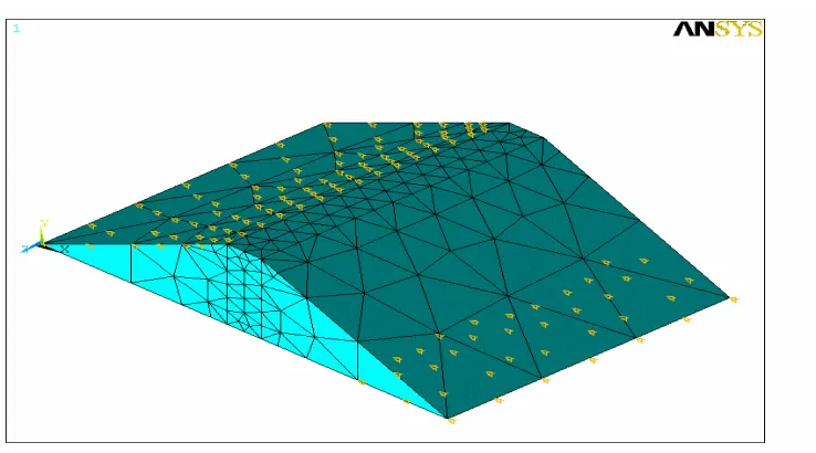
5, 6 and figure 7 As a result in three-dimensional analysis the length of the valley were assumed 100 meter.

In two-dimensional analysis, quadrilateral elements and triangular elements have been used, and boundary condition has been specified. In those places that higher integration order elements were needed, higher integration order elements were needed. Table (1) shows the details of a sample.

thermal solid element type has been used, which is called, SOLID87 3-D 10-Node tetrahedral thermal solid. It is well suited to model irregular meshes. The element has one degree of freedom, temperature, at each node. The element is applicable to a three-dimensional steady seepage analysis.

Results of the statistical analysis and especially regression are summarized in table 3. As shown in

the table, B represents the coefficient of the formula while;

β

shows the efficiency of the parameters. The letter further means that the most effective parameters would have the biggest

β

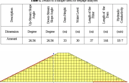
value. Parameters R and R2 represent the coefficient of correlation and the coefficient of determination respectively.

Figure 3. dam's geometrical parameters

Table 1. Details of a sample used for seepage analyses

Descri

p

tio

n

_Up-Strea

m Sl

o

p

e

An

gle

Down-St

ream

Sl

ope

A

n

gl

e

Dam Heig

ht

Water L

evel

Leng

th

o

f

th

e

Filter

Leng

th

o

f the

Dam

Hyd

rau

lic

Co

ndu

ctiv

ity

Dimension DegreeDegree (m) (m) (m) (m) (m/s)

Amount

26.56

26.56 33 30 37 144 1E-7

International Journal of Engineering Vol. 18, No. 2, May 2005 -191 Figure 5. 2-D analysis with SEEP/W software

Figure 6. 3-D modeling with ANSYS software

4. DISCUSSION AND ANALYSES

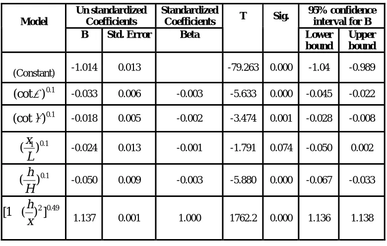
By using multiple regression (equation 12 and 13), the rate of seepage discharge is calculated from the models proposed. The results are illustrated in table 2 and 3. From table (2), it is clear that R2 and adjusted R2 are equal to one, which shows a very

exact regression. The equation that can estimate the flux is obtained from table (3) as follows:

49 . 0 2 1

. 0 1

. 0 1

1 . 0 1

. 0

] ) ( 1 [ 137 . 1 ) ( 05 . 0 ) ( 024 . 0

) (cot 018 . 0 ) (cot 033 . 0 014 . 1

x h H

h L

x kx

q

+ +

− −

− −

−

= α β

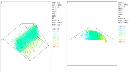
Figure7. 3-D analysis with ANSYS softwar

e

Table 2. Two-dimensional Model Summary

Change Statistics

R 2 _R

Adjuste

d

R

2

Std.

Error

of

The Estima

te

R

2

Ch

an

ge

F

Ch

an

ge

df1 df2

Sig. F _Chan

ge

Durbin

-

Watson

1.0 1.0 1.0 0.00755 1.0 1073132 5 593 0.0 1.626

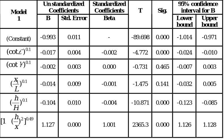
Considering the amount of the parameters, in three-dimensional analyses, multiple-regression has been performed. Results are illustrated in table 4 and table 5. From table 4, it is clear that R2 and adjusted R2 are equal to one, which shows a very exact regression. The equation that can estimate

the flux is obtained from table 5.

49 . 0 2 1

. 0 1

. 0 1

1 . 0 1

. 0

] ) ( 1 [ 127 . 1 ) ( 104 . ) ( 014 .

) (cot 002 . ) (cot 017 . 993 .

x h H

h L

x kx

q

+ +

−

− −

− −

= α β

International Journal of Engineering Vol. 18, No. 2, May 2005 -193 In equations (12) and (13): L= length of the dam,

(m), k=hydraulic conductivity, (m/s), H=height of dam, (m), h= water level, (m), x=distance between the horizontal filter blanket and the up-stream slope, (m),x₁=x+hcot

β

(m),

α

=down-stream slope angle,

β

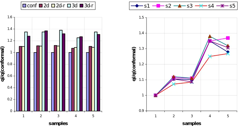
=up-stream slope angle

Comparison of the results showed in tables 3 and

5 shows that 3-D equation estimates the flux more than the 2-D equation. Five samples randomly selected are compared in table 6 which include summary of this comparison. Results are also graphically compared in Figure.8 which shows the difference between 2-D and 3-D crossing flux.

Table 3. Two-dimensional coefficients

Un standardized Coefficients

Standardized Coefficients

95% confidence interval for B Model

B Std. Error Beta

T Sig.

Lower bound

Upper bound

(Constant) -1.014 0.013 -79.263 0.000 -1.04 -0.989 1

. 0

)

(cot

α

-0.033 0.006 -0.003 -5.633 0.000 -0.045 -0.022

1 . 0

)

(cot

β

-0.018 0.005 -0.002 -3.474 0.001 -0.028 -0.008

1 . 0 1

)

(

L

x

-0.024 0.013 -0.001 -1.791 0.074 -0.050 0.002

1 . 0

)

(

H

h

-0.050 0.009 -0.003 -5.880 0.000 -0.067 -0.033

49 . 0 2

]

)

(

1

[

x

h

+

1.137 0.001 1.000 1762.2 0.000 1.136 1.138

Table 4. Three-dimensional Model Summary

Change Statistics

R 2 _R

Adj

u

ste

d

R

2

Std.

Error

of

The Estima

te

R

2 Chang

e

F

Ch

an

ge

df

1

df

2

Si

g. F Ch

ang

e

Durbin

-Watson

1.0

Table 5: Three-dimensional coefficients

Un standardized Coefficients

Standardized Coefficients

95% confidence interval for B Model

1 B Std. Error Beta

T Sig.

Lower bound

Upper bound

(Constant) -0.993 0.011 - -89.698 0.000 -1.014 -0.971

1 . 0

)

(cot

α

-0.017 0.004 -0.002 -4.772 0.000 -0.024 -0.010

1 . 0

)

(cot

β

_{-0.002 0.003 0.000 -0.731 0.465 -0.007 0.003}

1 . 0 1

)

(

L

x

-0.014 0.009 -0.001 -1.475 0.141 -0.032 0.005

1 . 0

)

(

H

h

-0.104 0.010 -0.004 -10.871 0.000 -0.123 -0.085

49 . 0 2

]

)

(

1

[

x

h

+

1.127 0.000 1.001 2365.3 0.000 1.126 1.128

5. COMPARING THE RESULTS

With comparing the results, it is clear that 3-D equation estimates the flux more than the 2-D

equation. 5 samples are compared with each other. Table 6shows these samples‘s information. Figure 7 and figure 8 illustrate the difference between 2-D and 3-D crossing flux.

Table 6. samples information

3-D 2-D Eq.12 Eq.13

L k H h

β

α

2.12E-03 1.73E-03 1.73E-03 2.01E-03

330 1E-5 300 225 63.43 63.43 Sample 1

1.33E-08 1.10E-08 1.09E-08 1.35E-08

162 1E-9 50 33 26.56 45.00 Sample 2

4.31E-05 3.49E-05 3.46E-05 4.12E-05

288 1E-6 108 65 45.00 33.69 Sample 3

2.89E-04 2.47E-04 2.50E-04 2.93E-04

417 5E-6 114 104 33.69 26.56 Sample 4

4.08E-08 3.34E-08 3.28E-08 3.95E-08

816 1E-9 132 99 18.43 18.43 Sample 5

(

s

m

2

) (

s

m

2

) (

s

m

2

) (

s

m

2

International Journal of Engineering Vol. 18, No. 2, May 2005 -195 Figure 8. comparing the results of conformal mapping techniques and the 2-D and 3-D analysis

6. CONCLUSION

In this paper, two and three-dimensional seepage of earth dams with horizontal filter blanket was studied. Some conclusions are drawn on the result of seepage discharge. In this study, there was a difference about 14-24% inseepage discharge rate between two and three-dimensional analysis, which is depend on the parameters such as water level and the up and dawn- stream slope angles and the length of dams

.

7. REFERENCES

1. Kashef, A.A.I. “Groundwater Engineering”, McGraw-Hill Book Company, New York, 1979, pp. 183-194.

2. Lacy, S.J. and Prevost, J.H., “Flow through porous media: A procedure for locating the free surface”, Intl. J. Num. Anal. Math. Geom., 1987, pp. 585-601.

3. Thieu, N.T.T., Fredlund, D.D. and Hung, V.Q., “General partial differential equation solvers for saturated-unsaturated seepage”, Proceeding of Unsaturated Soils for Asia, 2000, pp. 201-206 0

0.2 0.4 0.6 0.8 1 1.2 1.4 1.6

1 2 3 4 5

samples

qi

/q(conform

a

l)

conf 2d 2d-r 3d 3d-r

0.9 1 1.1 1.2 1.3 1.4 1.5

1 2 3 4 5

samples

qi/q(

c

onf

o

rm

a

l)