-

Wave Front Reconstruction from Off-Axis Holograms

Using Four-Quarter Phase Shifting Method

M. Hami,

*

A. Kiasatpour, and M. Soltanolkotabi

Quantum Optics Group, Department of Physics, Isfahan University, Isfahan, Islamic Republic of Iran

Abstract

In this paper a method for digitally recording four

quarter-reference-wave-holograms (by CCD) in a Mach-Zehnder interferometer setup, and reconstructing

the object wave-front by numerical method is presented. The terms of direct

transmission, auto-correlation and conjugate wave in the four wave reconstruction

are cancelled out and only one original object wave is left after overlapping.

Reconstructed digital holograms are obtained by computing the Fresnel-Kirchhoff

integral. Since the phase distribution of the wave field can be computed from the

digital hologram, one can measure micrometric displacements and deformations

of the reflecting object as well as small changes in refractive index field of the

transmission object. In order to calibrate a specially designed device necessary for

phase shifting purpose, we introduce a second Mach-Zehnder interferometer

inside the main imaging interferometer. With this second interferometer we can

directly observe displacement of a sector of circular interferometric fringes

without the presence of the (reflecting or transmitting) object. By simultaneously

transferring the images from the second interferometer to the computer and

recording the holograms we measure, using image processing, fringe displacement

in pixel units. Since the mirror on the phase shifting device is shared between two

interferometers, the measured optical path difference is automatically applied in

the main interferometer and thus the errors in shifting are substantially reduced.

Keywords: Digital holographic interferometry; Phase shifting; Image processing

*

E-mail: hamimohsen@yahoo.com Introduction

In the early 1970s Yaroslaskii et al. [1-3] initiated the numerical hologram reconstruction. The reconstruction algorithm was improved by Onural and Scott [4-6] and applied to particle measurements. A holographic microscope based on numerical reconstruction by Fourier holograms was described by Haddad et al. [7].

phases of the stored light waves can be calculated directly from the digital holograms, without generating phase-shifted interferograms [10]. Shearography and speckle photography can be preformed numerically from digital holograms [11].

The CCDs and other electronic devices for recording interferograms were already in use in electronic speckle pattern interferometry [12-13]. In this method two speckle interferograms are recorded at different states of the object under study and the speckle patterns are electronically subtracted. The resulting fringe pattern is almost similar to that of conventional or digital holographic interferometry, the main differences being the speckled appearance of the fringes and the loss of phase in the correlation process. The interference phase has to be recovered by an additional phase shifting process [14-15]. Digital holographic interferometry and electronic speckle pattern interferometry are two competing methods: the image subtraction in electronic speckle pattern interferometry is simpler than numerical reconstruction of digital holography, but there is more information in digital holograms. Electronic speckle pattern interferometry is not considered here [16-18].

Figure 1. Digitalholography (a) recording (b) reconstruction.

Figure 2. Coordinate system.

Sergio De Nicola et al. [19] have performed digital holographic interferometry only for a transmission object. They used a rotating glass plate for introducing the required phase shifts in recording holograms. They were able to suppress the zero order diffraction and the twin image. In the present work in addition to transmission object we have performed holographic interferometry of a reflection object and we were able to record speckled interferograms, in the process. In order to do the required phase shifting a mirror is mounted on a specially designed PZT device. A method is also introduced for the calibration of this device.

The General Principles of Digital Holography

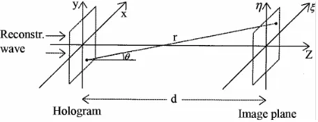
As shown in Figure (1-a) a plane reference wave and the wave reflected from a three dimensional object placed at a distance d from a CCD, interfere at the surface of the CCD. The resulting hologram is electronically recorded and stored. As shown in Figure (1-b) a virtual image appears at the position of the original object and the real image is formed also at a distance d, but in the opposite side from the CCD.

The diffraction of a light wave at CCD is described by the Fresnel-Kirchhoff integral [20]:

(

,

)

2 exp( ) ( , ) ( , )

1 1 cos 2 2

i i

h x y R x y

dxdy

ξ η

π ρ λ

λ ρ

θ

∞ ∞ −∞ −∞

Γ

− =

⎛ ⎞

×_⎜ + _⎟

⎝ ⎠

∫ ∫

(1)

where:

2 2 2

(x ) (y ) d

ρ= −ξ + −η + (2)

is the distance between a point in the hologram plane (CCD) and a point in the reconstruction plane as shown in Figure (2). For a plane reference wave:

R =r (3)

Knowing Γ

(

ξ η,

)

is important for numerical hologram reconstruction. In contrast to optical hologram reconstruction, in which only the intensity is made visible, here both the intensity and phase can be calculated [10].

2 2 2 2 3 2 2 ( ) ( ) 2 2 ( ) ( ) 1 ... 8 ( ) ( ) 2 2 x y d d d x y d x y d d d ξ η ρ ξ η ξ η − − = + + ⎡ − + − ⎤ ⎣ ⎦ − + − − ≈ + + (4)

with cosθ≈1 one obtains:

(

2 2

)

2

( , ) exp ( , ) ( , )

exp ( ) ( )

i

i d R x y h x y d

i

x y dxdy d

π ξ η

λ λ

π ξ η

λ

∞ ∞

−∞ −∞

⎛ ⎞

Γ _⎜− _⎟

⎝ ⎠ ⎡ ⎤ × _⎢− − + − _⎥ ⎣ ⎦

∫ ∫

2 2 2 2 2

exp( ) exp ( )

( , ) ( , ) exp ( )

i i

i d

d d

i

R x y h x y x y d

π _{π ξ η}

λ λ λ

π λ ∞ ∞ −∞ −∞ ⎡ ⎤ = − _⎢− + _⎥ ⎣ ⎦ ⎡ ⎤ × _⎢− + _⎥ ⎣ ⎦

∫ ∫

2

exp i (x y ) dxdy d

π _{ξ η} λ

⎡ ⎤

× _⎢ + _⎥

⎣ ⎦ (5)

This is called the Fresnel approximation [20]. It enables one to reconstruct the wavefield in a plane behind the hologram (CCD), in this case, in the plane of the real image.

The intensity and phase are calculated by:

2

( , )ξ η ( , )ξ η

Ι = Γ (6)

and

[

]

[

]

Im ( , ) ( , ) arctan

Re ( , )

ξ η ϕ ξ η

ξ η

Γ =

Γ (7)

respectively.

The virtual image reconstruction is also possible by introducing the imaging properties of a lens

(

_,

)

_exp

(

2 2

)

L x y i x y

f

π λ

⎡ ⎤

= _⎢ + _⎥

⎣ ⎦ into the numerical

reconstruction process [21]. This lens corresponds to the eye pupil of an observer watching through an optically reconstructed hologram. For unit magnification a focal distance of f =d/ 2 has to be used. The complex amplitude in the imaging plane is given by:

(

)

2 2 2

, i exp i d exp i ( )

d d

π π

ξ η ξ η

λ λ λ

⎛ ⎞ ⎡ ⎤

Γ = _⎜− _{⎟ ⎢}− + _⎥

⎝ ⎠ ⎣ ⎦

(

)

2 2

2 2

2 2

( , ) , ( , ) exp ( )

2

exp ( )

2

exp exp ( )

( , ) ( , ) exp ( )

2

exp ( )

i

R x y L x y h x y x y

d

i x y dxdy

d

i i

d i

d d

i

h x y R x y x y

d

i x y dxdy

d

π λ

π _{ξ η} λ

π _{π ξ η}

λ λ λ

π λ

π _{ξ η} λ ∞ ∞ −∞ −∞ ∞ ∞ −∞ −∞ ⎡ ⎤ × _⎢+ + _⎥ ⎣ ⎦ ⎡ ⎤ × _⎢ + _⎥ ⎣ ⎦ ⎛ ⎞ ⎡ ⎤ = _⎜− _{⎟ ⎢}− + _⎥ ⎝ ⎠ ⎣ ⎦ ⎡ ⎤ × _⎢+ + _⎥ ⎣ ⎦ ⎡ ⎤ × _⎢ + _⎥ ⎣ ⎦

∫ ∫

∫ ∫

(8)

By comparing (8) and (5), one sees only a change in the sign of the argument of the first exponential in the integrand.

Discrete Fresnel Transformation

To digitalize the Fresnel transform (5) the following substitutions are introduced:

d ξ ν λ = ; d η μ λ

= (9)

then (5) becomes:

[

]

2 2

2 2

( , ) exp ( )

( , ) ( , )

exp ( )

exp 2 ( )

i

i d d

R x y h x y

i

x y d

i x y dxdy

υ μ πλ υ μ

λ

π λ

π υ μ

∞ ∞

−∞ −∞

⎡ ⎤

Γ = _⎣− + _⎦

× ⎡ ⎤ × _⎢− + _⎥ ⎣ ⎦ × +

∫ ∫

(10)

this relation can be written as [20]:

2 2

1 2 2

( , ) exp ( )

( , ) ( , ) exp ( )

i

i d

d

i

R x y h x y x y

d

υ μ πλ υ μ

λ

π λ

−

⎡ ⎤

Γ = _⎣ + _⎦

⎧ ⎡ ⎤⎫

×ℑ ⎨ _⎢− + _⎥⎬

⎣ ⎦

⎩ ⎭

(11)

Now we are interested in digitalizing Γ. To do this the hologram function h x y

(

,

)

is sampled on a rectangular raster of N ×N points, with steps Δx and

y

The integrals in (10) are converted to finite sums:

[

]

2 2 2 2

1 1

0 0

2 2 2 2

( , ) exp ( )

( , ) ( , )

exp ( )

exp 2 ( )

N N

k l

i

m n i d m n

d

R k l h k l

i

k x l y

d

i k xm l yn

πλ υ μ

λ

π λ

π υ μ

− −

= =

⎡ ⎤

Γ = _⎣− Δ + Δ _⎦

×

⎡ ⎤

× _⎢− Δ + Δ _⎥

⎣ ⎦

× Δ Δ + Δ Δ

∑∑

for:

0,1,..., 1

m= N − and n =0,1,...,N −1 (12)

Using the Fourier transform theory, between Δx and υ

Δ and between Δy and Δμ the following relations exist:

1 1

and

N x N y

υ μ

Δ = Δ =

Δ Δ (13)

By introducing:

d d

and

N x N y

λ λ

ξ η

Δ = Δ =

Δ Δ (14)

the relation (12) converts to:

(

)

2 2

2 2 2 2

1 1

0 0

2 2 2 2

( , ) exp

( , ) ( , )] exp ln exp 2 N N k l

i m n

m n i d

d N x N y

R k l h k l

i k x l y d km i N N πλ λ π λ π − − = = ⎡ ⎛ ⎞⎤

Γ = _⎢− _⎜ + _⎟⎥

Δ Δ

⎝ ⎠

⎣ ⎦

×

⎡ ⎤

× _⎢− Δ + Δ _⎥

⎣ ⎦ ⎡ ⎛ ⎞⎤ × _{⎢ ⎜} + _⎟⎥ ⎝ ⎠ ⎣ ⎦

∑∑

(15)

The relation (15) is the discrete Fresnel transform and is the main relation that we are concerned with in this paper. In order to calculate the matrix Γ, we must multiply R k l

(

,

)

by h k l

(

,

)

and 2 2

exp[−iπ λ/ d k( Δx

2 2

)]

l y

+ Δ and then apply the inverse discrete Fourier transform to this product. The factor in front of the sum only affects the phase and can be neglected in most applications.

The terms of the intensity function resulting from the overlap of object and reference waves are cumbersome to deal with and therefore we introduce, in the flowing section, the four-quarter phase shifting method in order

to reduce the number of terms.

Four-Quarter Phase Shifting

Assume an object is placed at the distance d from the hologram plane. The object wave on the hologram plane is O x y

(

,

)

=o x y

(

,

)

exp

(

iϕ

(

x y,

)

)

. We use four reference plane waves that are in quadrature with one

another, namely, R1=rexp 0

( )

=r, ₂ exp 2

i R =r ⎛_⎜ π⎞_⎟=ir

⎝ ⎠ ,

( )

3 exp

R =r iπ = −r, ₄ exp 3 2

i

R =r ⎛_⎜ π⎞_⎟= −ir

⎝ ⎠ . Then we

can record four off-axis holograms with items [18]:

(

)

(

)

(

)

(

)

(

)

1

2 2 _{, , exp ,}

, exp ,

I r o x y ro x y i x y

ro x y i x y

ϕ ϕ = + + ⎡_⎣ ⎤_⎦ + ⎡_⎣− ⎤_⎦ (16-a)

(

)

(

)

(

)

(

)

(

)

2

2 2 _{, , exp ,}

, exp ,

I r o x y ro x y i x y

ro x y i x y

ϕ ϕ = + + ⎡_⎣ ⎤_⎦ + ⎡_⎣− ⎤_⎦ (16-b)

(

)

(

)

(

)

(

)

(

)

3

2 2 _{, , exp ,}

, exp ,

I r o x y ro x y i x y

ro x y i x y

ϕ

ϕ

= + + ⎡_⎣ ⎤_⎦

+ ⎡_⎣− ⎤_⎦ (16-c)

(

)

(

)

(

)

(

)

(

)

4

2 2 _{, , exp ,}

, exp ,

I r o x y ro x y i x y

ro x y i x y

ϕ

ϕ

= + + ⎡_⎣ ⎤_⎦

+ ⎡_⎣− ⎤_⎦

(16-d)

Illuminating the above four holograms, mathe-matically, with the corresponding reference waves, we have:

(

)

(

)

(

)

(

)

(

)

1 2 2

3 2 _, 1

, exp ,

, exp ,

R I r ro x y

r o x y i x y

r o x y i x y

ϕ ϕ = + + ⎡_⎣ ⎤_⎦ + ⎡_⎣− ⎤_⎦ (17-a)

(

)

(

)

(

)

(

)

(

)

2 2 2 2

3 2 _,

, exp ,

, exp ,

R I ir iro x y

r o x y i x y

r o x y i x y

ϕ ϕ − = + + ⎡_⎣ ⎤_⎦ − ⎡ ⎤ ⎣ ⎦ (17-b)

(

)

(

)

(

)

(

)

(

)

3 3 2 2

3 2 _,

, exp ,

, exp ,

R I r ro x y

r o x y i x y

r o x y i x y

(

)

(

)

(

)

(

)

(

)

4

4 2 2

3 2 _,

, exp ,

, exp ,

i

R I ir ro x y

r o x y i x y

r o x y i x y

ϕ

ϕ

−

−

= −

+ ⎡_⎣ ⎤_⎦

−

⎡ ⎤

⎣ ⎦

(17-d)

Adding Equations (17-a)- (17-d) together, we obtain:

(

)

(

)

1 1 2 2 3 3 4 4 2

4 , exp ,

R I R I R I R I

r o x y iϕ x y

+ + +

= ⎡_⎣ ⎤_⎦ (18)

As it can be seen the directly transmitting, auto-correlating, and conjugate terms in Equations(17-a)-(17-d) are cancelled out, leaving a term of pure wave front which, apart from a coefficient of 2

4r , is identical with the original object wave front. This term produces a virtual image in the original object position. If a positive lens with a focal length of d/2 is placed on the hologram plane, a real image can be generated on the other side, at a distance d from the hologram plane. On the other hand, if we choose R I1 1+R I4 2+R I3 3+R I2 4 we would

get 2

(

)

(

)

4r o x y, exp⎡_⎣−iϕ x y, ⎤_⎦. Thus the remaining term is the conjugate wave front which results in a real image on the other side at a distance d from the hologram plane without the aid of a lens.

Experiments and Results

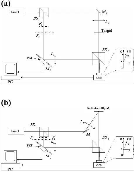
The geometrical arrangements used to record the transmission and the reflection objects are of different forms of Mach-Zehnder interferometers shown in Figures (3-a) and (3-b) respectively. He-Ne laser beam of wavelength 632.8 nm is split into an object beam and a reference beam by the beam splitter BS1(50%). The object beam is reflected from mirror M₁ and expanded by lens L1 of 10 mm focal length, after which it

illuminates the object. In the case of transmission the object is a slide with word "PHYSICS" typed on it, as shown in Figure (3-a). In the case of reflection, object is a metallic plate with the letters "IQOG" (Isfahan Quantum Optics Group) embossed on it Figure (3-b). The reference beam which in both cases passes a constant neutral filter F₁ and an incremental filter F₂ is reflected by the mirror M2 attached to piezoelectric

sheets (PZT) and passes through lens L₂ which is identical with the lens L1. These two beams come

together on the charge coupled device (CCD) by the second beam splitter BS2(50%). A Canon EOS300D camera with pixel size 4.5×4.5 µm2 is used to record the transmission object information and a Vixen video

camera with pixel size 6×6 µm2 is used for the reflection object. Both objects are located, in turns, at d=30 cm from CCD surface. The spatial angel θ is given by [22]:

2 x

λ θ <

Δ (19)

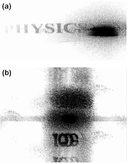
and is determined by pixel size (Δx ). This angel is adjusted by rotating BS₂ until interference fringes formed on the CCD surface become visible. Figures (4-a) and (4-b) show the holograms of the transmission and the reflection objects, respectively. Figure (4-b) shows the speckle interference pattern hologram, which every piece of it acts as the whole hologram. Figure (4-a) is the hologram of the transmission object and does not have the above property.

The reconstructed images of the two objects produced from the respective holograms are shown in Figures (5-a) and (5-b). Reconstruction is done through numerical calculation of equation (15) with the software MATLAB 6.5 making use of the following discrete two dimensional Fourier transform (FFT2) algorithm:

(a)

(b)

Figure 4. Holograms of (a) transmission object; (b) reflection object (speckle).

Figure 5. Reconstruction of one hologram: (a) transmission object; (b) reflection object.

(

)

( )

( )

( )

,

, , ,

n m j

A FFT R r s I r s EX P r s

ψ =

× ⎡_⎣ ⊗ ⊗ ⎤_⎦ (20)

( )

,

I r s is the recorded hologram intensity matrix which is determined by reading the hologram's image, using MATLAB. R r s

( )

, is the reference beam intensity matrix which is generated artificially in the computer program. The exponential term is actually

(

2 2 2 2

)

exp i r x s y

d

π λ

⎡ Δ + Δ ⎤

⎢ ⎥

⎢ ⎥

⎣ ⎦

which is calculated in two

loops in the program and stored as the matrix

( )

,

EX P r s . The first two terms in equation (15) are not considered for brevity of calculations and they cancel out anyway in intensity calculation. Also the two summations and the last exponential term are the discrete Fourier transform operations.

In order to eliminate the zero order diffraction image and the virtual image, we use four-quarter phase shifting. To produce a phase shift we make use of piezoelectric material. A second Mach-Zehnder interferometer is used for phase-shift calibration purposes. The shifts should be the stand in both interferometers. For this to be realized the mirror attached to the phase-shifter,M2, is shared in both

interferometers and the angles α and β are kept equal, as shown in Figure (6-a) and Figure (6-b). We have designed a programmable electronic hardware which introduces the required fringe shifts in the calibration interferometer as well as in the main interferometer. These fringe shifts are controlled by the computer using electronic device and video camera.

path variation produces macroscopic fringe shifts in the calibration interferometer. Now, when a bright fringe replaces a dark fringe which corresponds to reversal of the mean values in each matrix array, a path difference

of

4

λ _{(a phase shift of}

2

π _{) has occurred and it is time to}

record a new hologram. Using this technique four holograms are recorded in four phase stages, at phases

3 0, , ,

2 2

π _π π _.

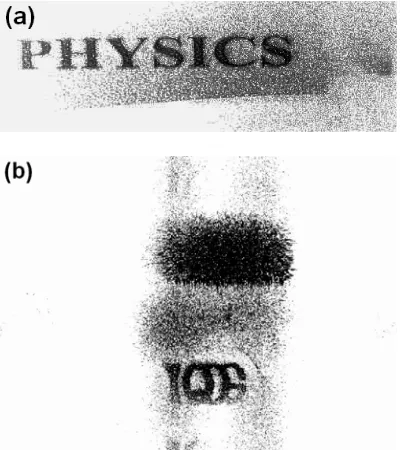
Combining these four holograms, using MATLAB as mentioned before, the final reconstructed image is obtained. Figures (8-a) and (8-b) show the final reconstructed image of the transmission and reflection objects, respectively. As it can be seen the zero order diffraction image, as well as the virtual image is eliminated (as compared with Figure (5-a) and (5-b)) and real images of the transmission and reflection objects are obtained.

a) b)

Figure 6. Geometrical arrangements for digital holography of (a) transmission object and calibration interferometer; (b) reflection object and calibration.

Figure 8. Reconstruction of holograms using Four-quarter phase shifting: (a) Transmission object; (b) Reflection object.

Summary

In this article digital holography of reflection and transmission objects are discussed. Holograms of such objects are digitally constructed and recorded. From these digital holograms the images of the objects are reconstructed and recorded. As in the case of optical holography, such reconstructions are accompanied by unwanted zero order and virtual images. In order to eliminate such images in our digitally recorded holographic reconstruction, we use the four-quarter phase shifting technique. An opto-mechanical phase shifter, a programmable electronic hardware which introduces the required shifts and a shift calibration device are designed in this work. Using these devices, four holograms are digitally recorded, each with a quarter wave shift. Combining these holograms, using MATLAB software, the final reconstructed image is recorded. In the final improved images the directly transmitting and conjugate images are absent.

In this technique, not only the three dimensional images are reconstructed, but the amount of roughness in the reflection object and refractive index profile in transmission object can be determined very accurately. Also very small (fraction of microns) in-plane and out-of-plane displacements, as well as, deformations in the objects can be determined.

Acknowledgements

The authors wish to thank the Office of Graduate Studies of University of Isfahan for its support.

Reference

1. Kronrod M.A., Yaroslavski L.P., and Merzlyakov N.S. Computer synthesis of transparency holograms. Sov. Phys.-Tech. Phys., 17: 329-332 (1980).

2. Kronrod M.A., Merzlyakov N.S., and Yaroslavski L.P. Reconstruction of holograms with a computer. Ibid., 17: 333-334 (1972).

3. Yaroslavski L.P. and Merzlyakov N.S. Methods of Digital Holography. New York: Consultants Bureau (1980). 4. Onural L. and Scott P.D. Digital decoding of in-line

holograms. Opt. Eng., 26: 1124-1132 (1987).

5. Liu G. and Scott P.D. Phase retrieval and twin-image elimination tor in-line Fresnel holograms. J. Opt. Soc. Am., A41: 59-65 (1987).

6. Onural L. and Ozgen M.T. Extraction of three-dimension-al object-location information directly from in-line holo-grams using Wigner analysis. Ibid., A9: 252-260 (1992). 7. Haddad W., Cullen D., Solem J.C., and Rhodes C.K.

Fourier-transform holographic microscope. Appl. Opt.,

31: 4973-4978 (1992).

8. Schnars U. and Juptner W. Principles of direct holography for interferometry FRINGE 93. In: Juptner W. and Osten W. (Eds.), Proc. 2nd Int. Workshop on Automatic Processing of Fringe Patterns, (Berlin: Akademie) pp. 115-120 (1993).

9. Schnars U. and Juptner W. Direct recording of holograms by a CCD-target and numerical reconstruction. Appl. Opt., 33: 179-181 (1994).

10. Schnars U. Direct phase determination in hologram intertferometry with use of digitally recorded holograms.

J. Opt. Sue. Am., A11: 2011-2015 (1994).

11. Schnars U. and Juptner W. Digital reconstruction of holograms in hologram interferometry and shearography.

Appl. Opt., 33: (1994).

12. Butters J.N. and Leendertz J.A. Holographic and video techniques applied to engineering measurements. J. Meas. Control, 4: 349-354 (1971).

13. Macovski A., Ramsey D., and Schaefer L.F. Time lapse interferometry and contouring using television systems.

Appl. Opt., 10: 2722-2727 (1971).

14. Stetson K.A. and Brohinsky R. Electronic holography and its application to hologram interferometry. Ibid., 24: 3631-3637 (1985).

15. Creath K. Phase shifting speckle interferometry. Ibid., 24: 3053-3058 (1985).

16. Lokberg O. Electronic speckle pattern interferometry.

Phys. Technol., 11: 16-22 (1980).

17. Lokberg O. and Slettemoen G.A. Basic electronic speckle pattern interferometry. Opt. Eng., 10: 455-505 (1987). 18. Rastogi P.K. Digital Speckle Pattern Interferometry and

Related Techniques.JohnWiley&Sons,pp.1-180(2001). 19. DeNicolaS.,FerraroP.,FinizioA.,and Pierattini G. Wave front reconstruction of Fresnel off-axis holograms with compensation of aberration by means of phase-shifting digital holography. Opt. Eng., 37: 331-340 (2002). 20. Goodman J.W. Introduction to Fourier Optics.

McGraw-Hill, New York (1968).

21. Harriharan P. Optical Holography. Cambridge: Cam-bridge University Press (1984).