The Thirty-Third AAAI Conference on Artificial Intelligence (AAAI-19)
Weighted Channel Dropout for
Regularization of Deep Convolutional Neural Network
Saihui Hou, Zilei Wang
Department of Automation, University of Science and Technology of China [email protected], [email protected]
Abstract
In this work, we propose a novel method named Weighted Channel Dropout (WCD) for the regularization of deep Con-volutional Neural Network (CNN). Different from Dropout which randomly selects the neurons to set to zero in the fully-connected layers, WCD operates on the channels in the stack of convolutional layers. Specifically, WCD consists of two steps,i.e., Rating Channels and Selecting Channels, and three modules,i.e., Global Average Pooling, Weighted Random Selection and Random Number Generator. It filters the channels according to their activation status and can be plugged into any two consecutive layers, which unifies the original Dropout and Channel-Wise Dropout. WCD is totally parameter-free and deployed only in training phase with very slight computation cost. The network in test phase remains unchanged and thus the inference cost is not added at all. Be-sides, when combining with the existing networks, it requires no re-pretraining on ImageNet and thus is well-suited for the application on small datasets. Finally, WCD with VGGNet-16, ResNet-101, Inception-V3 are experimentally evaluated on multiple datasets. The extensive results demonstrate that WCD can bring consistent improvements over the baselines.
Introduction
Recent years have witnessed the great bloom of deep Con-volutional Neural Network (CNN), which has significantly boosted the performance for a variety of visual tasks (He et al. 2016; Liu et al. 2016; Wang et al. 2016). The success of deep CNN is largely due to its structure of multiple non-linear hidden layers, which contain millions of parameters and thus are able to learn the complicated relationship be-tween input and output. However, when only limited train-ing data is available,e.g., in the field of Fine-grained Visual Categorization (FGVC), overfitting is very likely to occur, which would incur the performance drop.
In the previous literatures, many methods have been pro-posed to reduce the overfitting when training CNN, such as data augmentation, early stopping, L1 and L2 regularization, Dropout (Srivastava et al. 2014) and DropConnect (Wan et al. 2013). Among these methods, Dropout is one of the most popular which has been adopted in many classi-cal network architectures, including AlexNet (Krizhevsky,
Copyright c2019, Association for the Advancement of Artificial Intelligence (www.aaai.org). All rights reserved.
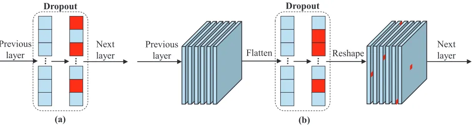
Sutskever, and Hinton 2012), VGGNet (Simonyan and Zis-serman 2014), and Inception (Szegedy et al. 2015; 2016). In Dropout, the output from the previous layer is flattened as a one-dimensional vector and a randomly selected subset of neurons is set to zero for the next layer (Figure 1). In most cases, Dropout is used to regularize the fully-connected lay-ers within CNN and not very suitable for the convolutional layers. One of the main reasons is that Dropout operates on each neuron, while in the convolutional layers each chan-nel consisting of multiple neurons is a basic unit that cor-responds to a specific pattern of input image (Zhang et al. 2016). In this work, we propose a novel regularization tech-nique for the stack of convolutional layers1which randomly selects channels for the next layer.
Another inspiration of this work comes from the ob-servation that in the stack of convolutional layers within CNN, all the channels generated by the previous layer are treated equally for the next layer. This is not optimal es-pecially for high layers where the features have greater specificity (Zeiler and Fergus 2014; Yosinski et al. 2014; Zhang et al. 2016). For each input image, only a few chan-nels in high layers are activated while the neuron responses in the other channels are close to zero (Zhang et al. 2016). So instead of totally random selection, we propose to select the channels according to the relative magnitude of activation status, which can be treated as a special way to model the interdependencies across the channels. To some extent, our work is similar in spirit to the recent SE-Block (Hu, Shen, and Sun 2017). The detailed comparison between our work and SE-Block will be provided below.
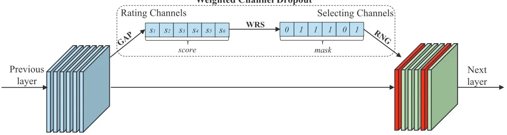
In summary, the main contribution of this work lies in a novel method named Weighted Channel Dropout (WCD) for the regularization of convolutional layers within CNN, which is illustrated in Figure 2. Notably the basic operation unit of WCD is the channel rather than the neuron. Specifi-cally, we first rate the channels output by the previous layer and assign ascorefor each channel. Thescoreis obtained by Global Average Pooling, which can acquire a global view of activation status in each channel. Second, regarding to the channel selection, a binarymaskis generated to indicate
1
Previous
layer Nextlayer
Dropout
Next layer Previous
layer
(a)
Dropout
(b)
Flatten Reshape
Figure 1: Illustration of Dropout. (a) Dropout in the fully-connected layers. (b) Dropout in the convolutional layers. The neurons in red are randomly selected and set to zero referring to the implementation in Caffe (Jia et al. 2014).
whether each channel is selected or not, and the channels with relatively high scores are kept with high probability. We find that the process of generating maskaccording to scorecan be boiled down to a special case of Weighted Ran-dom Selection (Efraimidis and Spirakis 2006) and an effi-cient algorithm is adopted for our purpose. Finally, a Ran-dom Number Generator is further attached tomaskto filter channels for the next layer. It is worth noting that, WCD is parameter-free and only added to the network in train-ing phase with very slight computation cost. The network in test phase remains unchanged and thus the inference cost is not added at all. Besides, WCD can be plugged into any ex-isting networks already pretrained on large-scale ImageNet and requires no re-pretraining, making it appealing for the application on small datasets.
The motivation of WCD is exactly to alleviate the overfit-ting of finetuning CNN on small datasets,e.g., the bulk of datasets for FGVC (Wah et al. 2011; Khosla et al. 2011; Krause et al. 2013; Maji et al. 2013), through adding more regularization to the stack of convolutional layers be-sides the fully-connected layers. For example, CUB-200-2011 (Wah et al. CUB-200-2011) collects only about30training im-ages for each class. By introducing more regularization, WCD can help the network learn more robust features from input. For the experiments, we evaluate WCD combin-ing with the classical networks includcombin-ing VGGNet-16 (Si-monyan and Zisserman 2014), ResNet-101 (He et al. 2016), Inception-V3 (Szegedy et al. 2016) on CUB-200-2011 (Wah et al. 2011) and Stanford Cars (Krause et al. 2013). Be-sides, for a thorough evaluation, we also evaluate WCD on Caltech-256 (Griffin, Holub, and Perona 2007) which fo-cuses on generic classification. The extensive results demon-strate that WCD can bring consistent improvements over the baselines.
Related Work
Due to the availability to large training data and GPU ac-celerated computation, multiple efforts have been taken to enhance CNN for greater capacity since the massive im-provement shown by AlexNet (Krizhevsky, Sutskever, and Hinton 2012) on ILSVRC2012. These efforts mainly con-sist of increased depth (Simonyan and Zisserman 2014;
He et al. 2016), enlarged width (Zagoruyko and Komodakis 2016), nonlinear activation (Maas, Hannun, and Ng 2013; He et al. 2015), reformulation of the connection between layers (Huang et al. 2017) and so on. Our method falls into the scope of adding regularization to neural networks. In this field, the previous works include Dropout (Srivastava et al. 2014), DropConnect (Wan et al. 2013), Batch Normal-ization (Ioffe and Szegedy 2015), DisturbLabel (Xie et al. 2016), Stochastic Depth (Huang et al. 2016) and so forth. Specifically, Dropout randomly selects a subset of neurons and sets them to zero, which is widely used for design-ing novel networks. DropConnect instead randomly sets the weights between layers to zero. Batch normalization im-proves the gradient propagation through network by normal-izing the input for each layer. DisturbLabel randomly re-places some labels with incorrect values to regularize the loss layer. Stochastic Depth randomly skips some layers in the residual networks. In addition, (Park and Kwak 2016) analyze the effect of Dropout on max-pooling and convo-lutional layers. (Morerio et al. 2017) extend the standard Dropout by introducing a time schedule to adaptively in-crease the ratio of dropped neurons.
Among these works, Dropout (Srivastava et al. 2014) is the most popular and more related to our method. Both work by randomly setting a portion of responses of hidden layers to zero in the training. However, there exist clear differences between WCD and Dropout. First, WCD is proposed to reg-ularize the stack of convolutional layers while Dropout is usually inserted between the fully connected layers. Second, WCD differs from Dropout in that it operates on the chan-nels other than the neurons. While in the stack of convolu-tional layers, each channel is a basic unit. Finally, the neu-ron selection in Dropout is completely random, in contrast, WCD selects the channels according to their activation sta-tus. Actually, Dropout can be seen as a special case of WCD, which will be discussed below. Both WCD and Dropout can be combined in one network, which is exactly the practice in our experiments.
rela-Weighted Channel Dropout
Next layer Previous
layer
Rating Channels Selecting Channels
WRS
score mask
s1 s2 s3 s4 s5 s6 0 1 1 1 0 1
Figure 2: Illustration of Weighted Channel Dropout.GAP: Global Average Pooling,WRS: Weighted Random Selection,RNG: Random Number Generator. The channels are selected according to the activation status. The red ones are set to zero and the green are rescaled from the corresponding input channels.
tive magnitude of activation status, WCD can be treated as a special way to explore the channel relationship, which is the focus of SE-Block. However, compared to SE-Block, first of all, WCD is totally parameter-free and added only in train-ing phase, thus leavtrain-ing the inference cost not added at all. Second, when combining SE-Block with the existing net-works, it requires re-pretraining the whole model on large-scale ImageNet before finetuning on other datasets. Unlike SE-Block, WCD can be plugged into any existing networks and does not need to re-pretrain the whole model, thus fit-ting well for the application on small datasets. Finally, WCD is usually applied to high convolutional layers within CNN while SE-Block mainly affects early convolutional layers. From this perspective, WCD and SE-Block are complemen-tary to each other.
Our Approach
WCD is designed to provide regularization to the stack of convolutional layers within CNN. Taking VGGNet (Si-monyan and Zisserman 2014) as an example, Dropout is inserted among the last three fully-connected layers, while no regularization is deployed in the layers before pool5. When finetuning VGGNet on small datasets, more regu-larization is wished since the overfitting is severe. Here we present some notations which will be used in the fol-lowing. Formally, in two consecutive convolutional layers,
X = [x1, x2,· · · , xN]denotes the output of previous layer,
e
X = [xe1,xe2,· · ·,exNe]denotes the input to next layer, N
andNe are the number of channels, xi andexi are thei-th channel. In almost all cases,Xe =X,i.e., there areNe =N and
e
xi=xi, i= 1,2,· · ·, N (1)
Differently, WCD randomly selects the channels fromXto constructXeaccording to the activation status in each chan-nel. It is worth noting that the previous or the next layer could also be pooling layer and so on. Without loss of gen-erality, here we discuss the case of two consecutive convo-lutional layers. Next we will present the details of WCD, which consists of two steps (i.e., Rating Channels and
Se-lecting Channels) and three modules (i.e., Global Average Pooling, Weighted Random Selection and Random Number Generator). In our method, we still haveNe =N.
Step 1: Rating Channels
According to the observation in previous works (Zeiler and Fergus 2014; Yosinski et al. 2014; Zhang et al. 2016), the features in high layers of CNN have great specificity (i.e., class-specific in the context of image classification) and only a small fraction of channels are activated for each input im-age (Zhang et al. 2016). Thus, instead of treating all channels equally and conducting random selection, we propose to first rate the channels and assign each channel ascore, which is used as the guidance for channel selection in the following step.
Global Average Pooling (GAP). In deep CNN, a neuron in high layers corresponds to a local patch in the input im-age and a channel consisting of multiple neurons represents a specific pattern (Zhang et al. 2016). In order to rate each channel, we adopt a simple but effective method,i.e., Global Average Pooling, to acquire a global view of activation sta-tus in each channel. Formally,
scorei= 1
W ×H
W X
j=1 H X
k=1
xi(j, k) (2)
whereW andHare the shared width and height of all chan-nels. There are more sophisticated strategies (S´anchez et al. 2013; Yang et al. 2009; Lin, RoyChowdhury, and Maji 2015; Gao et al. 2016) to obtain thescorewhich need further ex-ploration. It is normal to assume that scorei > 0 since ReLU is appended behind each convolutional layer in mod-ern CNNs (Simonyan and Zisserman 2014; He et al. 2016; Szegedy et al. 2016).
Step 2: Selecting Channels
Algorithm 1Weighted Random Selection
Input: scorei > 0, maski = 0, i = 1,2,· · · , N, wrs ratio.
Output: maski, i = 1,2,· · · , N. The probability of
maski= 1ispi= scorei
PN
j=1scorej.
1: For eachi,ri=random(0,1)andkeyi=r
1
scorei
i .
2: Select theM =N ∗wrs ratioitems with the largest keyiand set the correspondingmaskito1.
maskito indicate whetherxiis kept or not. The probability piof keeping the channelxiis set to
pi=
scorei
PN
j=1scorej
(3)
That is to say,maski has the probabilitypi to be set to1, and the channels with relatively highscoresare more likely to be kept. In the following we will present the algorithm to achieve this goal, taking the computation cost and efficiency into account.
Weighted Random Selection (WRS). We find that the process of generating mask according to score can be boiled down to a special case of Weighted Random Selec-tion (Efraimidis and Spirakis 2006). An efficient algorithm is adopted for our purpose, which is illustrated in Algo-rithm 1. Specifically, first, for channelxiwithscorei, a ran-dom numberri∈(0,1)is generated and a key valuekeyiis computed as
keyi=r
1
scorei
i (4)
ThenM items with the largest key values are selected and the correspondingmaskiare set to1. Herewrs ratio=MN is a hyper-parameter of WCD, indicating how many chan-nels are kept after WRS. The algorithm is computationally efficient, which can setmaskito1with the probabilitypi shown in Equation 3. Please refer to (Efraimidis and Spi-rakis 2006) for more details about the algorithm.
Random Number Generation (RNG). Going further, for small datasets, the training usually starts from the models pretrained on ImageNet instead of from scratch. In high con-volutional layers within the pretrained model, the disparity between channels is large,i.e., only a few channels are as-signed relatively high activation values with the others close to zero (Zhang et al. 2016). If we totally select channels according toscorein these layers, it is possible that for a given image, the sequence of selected channels is basically the same in each forward process2, which is not desired. To alleviate this, we further propose to add a binary Random Number Generatorrngwith the parameterqtomaski. Thus in the case thatmaskiis set to1,xistill has the probability
1−qto be not selected.
2
For example, suppose thatpipj,∀j6=i,maskiis almost certain to be set to1
Pool5
GAP
WRS
RNG
Filter
WCD
Flatten
FC6
(a)
Residual
GAP
WRS
RNG
WCD
Filter
(b)
Inception
GAP
WRS
RNG
Filter
WCD
(c)
Figure 3: The schema to combine WCD with the existing networks. (a) WCD with VGGNet. (b) WCD with ResNet. (c) WCD with Inception.
Summary
On the whole,Xe is constructed as follows:
e
xi=
αxi if maski= 1and rng= 1
0 otherwise (5)
wheremaskihas the probabilitypito be set to1,rng gen-erates1 with the probability q,xie = 0means that all the neurons in itsW×Hzone are set to zero. The coefficientα is used to reduce the bias between training and test data. In our implementation,αis empirically set to
α=
PN
j=1scorej P
j∈Mfscorej
(6)
whereMfdenotes the set of channels which are finally se-lected, the numerator is to sum the scoresof all channels and the denominator is to sum thescoresof selected chan-nels. WCD is added only in training phase, while at infer-ence time, all channels are sent into the next layer.
Moreover, letkeep ratiodenote the ratio of how many channels are kept forXein training3, and we have
keep ratio=|Mf|
N ≈wrs ratio×q (7)
where|Mf|denotes the number of elements inMf,wrs ratio andqare two hyper-parameters of WCD. Usually we have
0 < wrs ratio < 1 and0 < q < 1. Besides, WCD also unifies the following special cases:
1. wrs ratio = 1,0 < q < 1.Xe is constructed by totally random selection from the channels inX, which is de-noted as Channel-Wise Dropout. WhenW =H = 1, it is equivalent to the original Dropout.
2. 0< wrs ratio <1, q= 1. The channels withmaski= 1will be surely kept.
The cases that either wrs ratio or q is set to 0 make no sense. WCD can be also treated as a more generic version
3
(a)
(b)
(c)
Figure 4: Example images. (a) CUB-200-2011. (b) Stanford Cars. (c) Caltech-256.
of Channel-Wise Dropout and brings additional flexibility. For instance, since the channels with highscoresare more likely to be selected, the selected channels remain discrimi-native even with a lowkeep ratioand would not hinder the convergence of network.
Application
WCD can be theoretically plugged into any two consecu-tive layers within CNN. In practice, it is usually used to regularize the stack of convolutional layers. The schema to integrate WCD with the classical networks including VG-GNet (Simonyan and Zisserman 2014), ResNet (He et al. 2016) and Inception (Szegedy et al. 2016) are displayed in Figure 3. Specifically, inspired by the observation that the channels in early convolutional layers are more related to each other (Tompson et al. 2015) , we mainly deploy WCD behind the high layers, such aspool4andpool5in VGGNet-16, res5a and res5c in ResNet-101. To stress again, as a lightweight parameter-free module, WCD is added to these networks only in training phase and the network in test phase is unchanged. Besides, it requires no re-pretaining on Ima-geNet and thus can be easily deployed when finetuning these networks on small datasets.
Experiment
Experimental Setup
In this section, we evaluate WCD combining with VGGNet-16 (Simonyan and Zisserman 2014), ResNet-101 (He et al. 2016), Inception-V3 (Szegedy et al. 2016) on CUB-200-2011 (Wah et al. CUB-200-2011), Stanford Cars (Krause et al. 2013) and Caltech-256 (Griffin, Holub, and Perona 2007). On these datasets, the scale of training set is rather small and thus overfitting is more likely to occur.
All the models are implemented with Caffe (Jia et al. 2014) on Titan-X GPUs. WCD is added to the networks in training phase with the original layers remaining unchanged. The hyper-parameters includingwrs ratioandqare set by cross validation and keep consistent on the similar datasets
Table 1: The parameter settings of WCD on CUB-200-2011 and Stanford Cars.
VGGNet-16 ResNet-101 Inception-V3
layer 1 pool4 res5a reduction b
wrs ratio1 0.8 0.8 0.8
q 1 0.9 0.9 0.9
layer 2 pool5 res5c inception c2
wrs ratio2 0.9 0.8 0.8
q 2 0.5 0.9 0.9
Table 2: The performance comparison on CUB-200-2011 and Stanford Cars.
CUB Cars
VGGNet-16 72.31% 86.11%
WCD-VGGNet-16 76.10% (+3.79%) 88.28% (+2.17%)
ResNet-101 76.45% 87.84%
WCD-ResNet-101 77.22% (+0.77%) 88.37% (+0.53%)
Inceptin-V3 83.98% 93.17%
WCD-Inception-V3 84.52% (+0.54%) 93.41% (+0.24%)
such as CUB-200-2011 and Stanford Cars. The training starts from the model pretrained on ImageNet. Stochastic gradient descent (SGD) is used for the optimization. The ini-tial learning rate is set to 0.001 and reduces to its 1/10 three times until convergence. In all experiments, the images are randomly flipped and cropped before passing into the net-works, and no other data augmentation is used. The infer-ence is done with one center crop of the test images. Finally, the top-1 accuracy is taken as the metric for evaluation.
CUB-200-2011 & Stanford Cars
CUB-200-2011 (Wah et al. 2011) is a widely-used fine-grained dataset which collects images in 200 birds species. For each class, there are about 30 images for training. Some example images are shown in Figure 4(a).
VGGNet-16, ResNet-101, Inception-V3 are adopted as the baselines. The parameters of integrating WCD with these networks are shown in Table 1. For all three networks, WCD is deployed behind the last two layers conducting the fea-ture dimension reduction in the stack of convolutional lay-ers, e.g.,pool4andpool5in VGGNet-16, res5aandres5c in ResNet-101. Please refer to (Simonyan and Zisserman 2014), (He et al. 2016) and (Szegedy et al. 2016) for the details of network structures. As shown in Table 2, WCD can bring consistent improvements over the baselines. For VGGNet-16, WCD achieves a significant 3.79% improve-ment over the base model.
base-Table 3: The parameter settings of WCD and performance comparison on Caltech-256.*-reported on the reduced test set consisting of 20 images per class.
VGGNet-16 ResNet-101 Inception-V3
layer 1 pool5 res5c inception c2
wrs ratio1 0.8 0.8 0.8
q1 0.9 0.9 0.9
Baseline 72.31% 78.00% 79.52%
With WCD 72.86% 78.30% 80.61%
(+0.55%) (+0.30%) (+1.09%)
Baseline* 70.91% 77.28% 78.81%
With WCD* (+0.92%71.83%) (+0.66%77.94%) (+1.11%79.92%)
lines are relatively high, while the models with WCD still consistently outperform the baselines.
Discussion.The recent work (Zheng et al. 2017) lists the performance reported on CUB-200-2011 and Stanford Cars, where the methods can be roughly divided into two cate-gories. The first one is to encode CNN features for more discriminative representation, such as Bilinear CNN (Lin, RoyChowdhury, and Maji 2015) and Compact Bilinear CNN (Gao et al. 2016). The second is to exploit the at-tention mechanism, such as RA-CNN (Fu, Zheng, and Mei 2017) and MA-CNN (Zheng et al. 2017). Our method does not belong to either of the above categories and the focus of this paper is not to report state-of-the-art performance. WCD is a fairly generic method to alleviate the overfitting when finetuning CNN on small datasets, which can be integrated into these existing models. We take some preliminary exper-iments to combine WCD with Compact Bilinear CNN (Gao et al. 2016), and find that WCD can help outperform this strong baseline (84.88%vs.84.01%)4.
Caltech-256
Both CUB-200-2011 and Stanford Cars belong to the field of fine-grained visual categorization. In order to obtain a thorough evaluation of WCD, here we further evaluate it on Caltech-256 (Griffin, Holub, and Perona 2007) which focuses on generic classification. Some example images of Caltech-256 are shown in Figure 4(c), which display larger inter-class difference than fine-grained datasets. There is no split way provided in the dataset, and for each class we ran-domly select 20 images for training with the rest as test set. The experimental settings are a little different from those on CUB-200-2011 and Stanford Cars. Specifically, WCD is appended behind the last layer conducting the feature di-mension reduction in the stack of convolutional layers, such aspool5in VGGNet-16,res5cin ResNet-101. The perfor-mance comparison as well as the parameter details is shown in Table 3. It can be seen that, WCD also works well on Caltech-256 and helps achieve superior performance over the base model.
Discussion.We notice that Caltech-256 (Griffin, Holub,
4
WCD is added afterpool5with the other settings unchanged.
Table 4: The ablation study of WCD. The results are re-ported on CUB-200-2011.
Approach Settings Accuracy
A
VGGNet-16 baseline 72.31%
B VGGNet-16+
pool5Dropout dropout ratio= 0.5 73.90%
C
VGGNet-16+ pool5SE-Block
SE-Block not pretrained 72.71%
D SE-Block pretrained 73.05%
E VGGNet-16+ pool5WCD
wrs ratio= 0.9
q= 0.5 75.60%
F
VGGNet-16+ pool5WCD
wrs ratio= 1
q= 0.45 75.02%
G wrs ratio= 0.45
q= 1 73.28%
H wrs ratio= 0.9
q= 0.5 75.60%
I
VGGNet-16+ pool5WCD
wrs ratio= 1
q= 0.25 73.16%
J wrs ratio= 0.25
q= 1 72.16%
K wrs ratio= 0.5
q= 0.5 75.33%
and Perona 2007) exhibits long-tail distribution where the number of images for each class largely varies from each other. Thus we further report the results on the reduced test set containing the same number of images for each class. Specifically, the training set remains unchanged, and we ran-domly select another 20 images from each class as the test set which has no overlap with the training set. The perfor-mance comparison is shown in the last two rows of Table 3, which further validate the effectiveness of WCD.
Ablation Study
In this subsection, we take extensive experiments to analyze the behaviors of WCD.
Channel dropout analysis.WCD is based on the obser-vation that in high convolutional layers of CNN (pretrained on ImageNet or finetuned on the specific dataset), for an in-put image, only a few channels are activated with relatively high values while the neuron responses in the other channels are close to zero. The phenomenon is validated by the exper-iments in (Zhang et al. 2016). Noticing that the experexper-iments in (Zhang et al. 2016) were performed on image patches, we conduct the similar experiments on full images and get the same observations. For example, for the input images ran-domly selected from CUB-200-2011, nearly half of chan-nels in thepool5of VGGNet-16 hold the responses that are zero or very close to zero.
Iteration
0 2500 5000 7500 10000
Top-1 error
0 0.2 0.4 0.6 0.8 1
train error without WCD test error without WCD train error with WCD test error with WCD
Figure 5: Effect of WCD on network training. The exper-iments are conducted on CUB-200-2011 with VGGNet-16 as the base model. Best viewed in color.
dataset from the pretrained model on ImageNet. Then, given that SE-Block contains two fully-connected layers, we fur-ther re-pretrain the whole model on ImageNet before fine-tuning on small datasets. The resulting accuracy is a little better than that without re-pretraining, but still inferior to that with WCD (Row E).
Special cases of WCD.Row F and Row G of Table 4 are the two special cases of WCD as aforementioned,i.e., either
wrs ratioorqis set to 1. The comparison between Row F
and Row H shows the effectiveness of WCD compared to Channel-wise Dropout, while the comparison between Row G and Row H indicates the necessity of RNG in WCD. Be-sides, the results in the last three rows of Table 4 further demonstrates the superiority of WCD, indicating that WCD enables a lowkeep ratio(≈wrs ratio×q= 0.25). It may suit for the cases where the training images are very rare, such as in medical image analysis (Qayyum et al. 2017).
Effect on network training.Figure 5 shows the effect of WCD on training with the settings shown in Table 1. It can be seen that, the curve of training error with WCD drops more slowly while the resulting test error is lower, proving that WCD can reduce overfitting in the training phase.
Computation cost of WCD.Table 5 provides some com-plexity statistics of WCD, which indicates that the compu-tation cost introduced by WCD is negligible. Besides, these additional cost is introduced only in training phase and the inference cost is not increased at all.
Conclusion
In this work, we deal with the regularization of CNN by proposing a novel method named WCD for the stack of con-volutional layers. Specifically, WCD filters the channels ac-cording to their activation status for the next layer. It consists of two steps,i.e., Rating Channels and Selecting Channels,
Table 5: Computation cost introduced by WCD. The statis-tics are obtained on a Titan GPU withbatch size= 32. The training time is averaged over the first 100 iterations.
GPU memory (MB)
Training time (sec/iter)
VGGNet-16 5753 0.74
WCD-VGGNet-16 5817 0.83
and three modules,i.e., Global Average Pooling, Weighted Random Selection and Random Number Generator. As a whole, WCD is a lightweight component which can be inte-grated into any existing models with negligible computation cost introduced only in training phase. Its characteristics, e.g., parameter-free and no need to re-pretrain on ImageNet, make it well-suited for the application on small datasets. Finally, the experimental results with VGGNet-16, ResNet-101, Inception-V3 on multiple datasets show the robustness and superiority of WCD. For the future work, we plan to apply WCD to other types of visual tasks, such as object detection.
Acknowledgment
This work is supported by the National Natural Science Foundation of China under Grant 61673362 and 61836008, Youth Innovation Promotion Association CAS (2017496), and the Fundamental Research Funds for the Central Uni-versities.
References
Efraimidis, P. S., and Spirakis, P. G. 2006. Weighted random sam-pling with a reservoir. Information Processing Letters97(5):181– 185.
Fu, J.; Zheng, H.; and Mei, T. 2017. Look closer to see better: Recurrent attention convolutional neural network for fine-grained image recognition. InCVPR.
Gao, Y.; Beijbom, O.; Zhang, N.; and Darrell, T. 2016. Compact bilinear pooling. InCVPR.
Griffin, G.; Holub, A.; and Perona, P. 2007. Caltech-256 object category dataset. Technical Report 7694, California Institute of Technology.
He, K.; Zhang, X.; Ren, S.; and Sun, J. 2015. Delving deep into rectifiers: Surpassing human-level performance on imagenet clas-sification. InICCV.
He, K.; Zhang, X.; Ren, S.; and Sun, J. 2016. Deep residual learn-ing for image recognition. InCVPR.
Hu, J.; Shen, L.; and Sun, G. 2017. Squeeze-and-excitation net-works.arXiv preprint arXiv:1709.01507.
Huang, G.; Sun, Y.; Liu, Z.; Sedra, D.; and Weinberger, K. Q. 2016. Deep networks with stochastic depth. InECCV.
Huang, G.; Liu, Z.; van der Maaten, L.; and Weinberger, K. Q. 2017. Densely connected convolutional networks. InCVPR. Ioffe, S., and Szegedy, C. 2015. Batch normalization: Accelerat-ing deep network trainAccelerat-ing by reducAccelerat-ing internal covariate shift. In ICML.
Convo-lutional architecture for fast feature embedding. arXiv preprint arXiv:1408.5093.
Khosla, A.; Jayadevaprakash, N.; Yao, B.; and Li, F.-F. 2011. Novel dataset for fine-grained image categorization: Stanford dogs. In CVPR Workshop.
Krause, J.; Stark, M.; Deng, J.; and Fei-Fei, L. 2013. 3d object representations for fine-grained categorization. InICCV Workshop. Krizhevsky, A.; Sutskever, I.; and Hinton, G. E. 2012. Imagenet classification with deep convolutional neural networks. InNIPS. Lin, T.-Y.; RoyChowdhury, A.; and Maji, S. 2015. Bilinear cnn models for fine-grained visual recognition. InICCV.
Liu, W.; Anguelov, D.; Erhan, D.; Szegedy, C.; Reed, S.; Fu, C.-Y.; and Berg, A. C. 2016. Ssd: Single shot multibox detector. In ECCV.
Maas, A. L.; Hannun, A. Y.; and Ng, A. Y. 2013. Rectifier nonlin-earities improve neural network acoustic models. InICML. Maji, S.; Rahtu, E.; Kannala, J.; Blaschko, M.; and Vedaldi, A. 2013. Fine-grained visual classification of aircraft. arXiv preprint arXiv:1306.5151.
Morerio, P.; Cavazza, J.; Volpi, R.; Vidal, R.; and Murino, V. 2017. Curriculum dropout. InICCV.
Park, S., and Kwak, N. 2016. Analysis on the dropout effect in convolutional neural networks. InACCV.
Qayyum, A.; Anwar, S. M.; Majid, M.; Awais, M.; and Alnowami, M. 2017. Medical image analysis using convolutional neural net-works: A review.arXiv preprint arXiv:1709.02250.
S´anchez, J.; Perronnin, F.; Mensink, T.; and Verbeek, J. 2013. Im-age classification with the fisher vector: Theory and practice. In-ternational Journal of Computer Vision105(3):222–245.
Simonyan, K., and Zisserman, A. 2014. Very deep convolu-tional networks for large-scale image recognition. arXiv preprint arXiv:1409.1556.
Srivastava, N.; Hinton, G.; Krizhevsky, A.; Sutskever, I.; and Salakhutdinov, R. 2014. Dropout: a simple way to prevent neu-ral networks from overfitting. The Journal of Machine Learning Research15(1):1929–1958.
Szegedy, C.; Liu, W.; Jia, Y.; Sermanet, P.; Reed, S.; Anguelov, D.; Erhan, D.; Vanhoucke, V.; and Rabinovich, A. 2015. Going deeper with convolutions. InCVPR.
Szegedy, C.; Vanhoucke, V.; Ioffe, S.; Shlens, J.; and Wojna, Z. 2016. Rethinking the inception architecture for computer vision. InCVPR.
Tompson, J.; Goroshin, R.; Jain, A.; LeCun, Y.; and Bregler, C. 2015. Efficient object localization using convolutional networks. InCVPR.
Wah, C.; Branson, S.; Welinder, P.; Perona, P.; and Belongie, S. 2011. The caltech-ucsd birds-200-2011 dataset. Technical Report CNS-TR-2011-001, California Institute of Technology.
Wan, L.; Zeiler, M.; Zhang, S.; Cun, Y. L.; and Fergus, R. 2013. Regularization of neural networks using dropconnect. InICML. Wang, L.; Xiong, Y.; Wang, Z.; Qiao, Y.; Lin, D.; Tang, X.; and Van Gool, L. 2016. Temporal segment networks: towards good practices for deep action recognition. InECCV.
Xie, L.; Wang, J.; Wei, Z.; Wang, M.; and Tian, Q. 2016. Distur-blabel: Regularizing cnn on the loss layer. InCVPR.
Yang, J.; Yu, K.; Gong, Y.; and Huang, T. 2009. Linear spatial pyramid matching using sparse coding for image classification. In CVPR.
Yosinski, J.; Clune, J.; Bengio, Y.; and Lipson, H. 2014. How transferable are features in deep neural networks? InNIPS. Zagoruyko, S., and Komodakis, N. 2016. Wide residual networks. InBMVC.
Zeiler, M. D., and Fergus, R. 2014. Visualizing and understanding convolutional networks. InECCV.
Zhang, X.; Xiong, H.; Zhou, W.; Lin, W.; and Tian, Q. 2016. Pick-ing deep filter responses for fine-grained image recognition. In CVPR.