Modular Proximal Optimization for Multidimensional
Total-Variation Regularization
´
Alvaro Barbero [email protected]
Instituto de Ingenier´ıa del Conocimiento and Universidad Aut´onoma de Madrid Francisco Tom´as y Valiente 11, Madrid, Spain
Suvrit Sra∗ [email protected]
Laboratory for Information and Decision Systems
Massachusetts Institute of Technology (MIT), Cambridge, MA
Editor:Vishwanathan S V N
Abstract
We studyTV regularization, a widely used technique for eliciting structured sparsity. In particular, we propose efficient algorithms for computing prox-operators for`p-norm TV.
The most important among these is`1-norm TV, for whose prox-operator we present a new geometric analysis which unveils a hitherto unknown connection to taut-string methods. This connection turns out to be remarkably useful as it shows how our geometry guided im-plementation results in efficient weighted and unweighted 1D-TV solvers, surpassing state-of-the-art methods. Our 1D-TV solvers provide the backbone for building more complex (two or higher-dimensional) TV solvers within a modular proximal optimization approach. We review the literature for an array of methods exploiting this strategy, and illustrate the benefits of our modular design through extensive suite of experiments on (i) image denois-ing, (ii) image deconvolution, (iii) four variants of fused-lasso, and (iv) video denoising. To underscore our claims and permit easy reproducibility, we provide all the reviewed and our new TV solvers in an easy to use multi-threaded C++, Matlab and Python library. Keywords: proximal optimization, total variation, regularized learning, sparsity, non– smooth optimization
1. Introduction
Sparsity impacts the entire data analysis pipeline, touching algorithmic, modeling, as well
as practical aspects. Most commonly, sparsity is elicited via `1-norm regularization
(Tib-shirani, 1996; Cand`es and Tao, 2004). However, numerous applications rely on more refined
“structured” notions of sparsity, e.g., groupwise-sparsity (Meier et al., 2008; Liu and Zhang, 2009; Yuan and Lin, 2006; Bach et al., 2011), hierarchical sparsity (Bach, 2010; Mairal et al., 2010), gradient sparsity (Rudin et al., 1992; Vogel and Oman, 1996; Tibshirani et al., 2005), or sparsity over structured ‘atoms’ (Chandrasekaran et al., 2012).
Such regularizers typically arise in optimization problems of the form
minx∈Rn Φ(x) :=`(x) +r(x), (1.1)
∗. An initial version of this work was performed during 2013-14, when the author was with the Max Planck Institute for Intelligent Systems, T¨ubingen, Germany, and with Carnegie Mellon University, Pittsburgh.
c
where `:Rn→R is a smooth loss function (often convex), while r :Rn→ R∪ {+∞}is a lower semicontinuous, convex, and nonsmooth regularizer that induces sparsity.
We focus on instances of (1.1) where r is a weighted anisotropic Total-Variation (TV)
regularizer1, which for a vectorx∈Rn and fixed weightsw≥0 is defined as
r(x) def= Tv1p(w;x) def= Xn−1
j=1wj|xj+1−xj|
p1/p p≥1. (1.2)
More generally, ifX is an order-m tensor inR
Qm
j=1nj with entriesX
i1,i2,...,im (1≤ij≤nj for
1≤j ≤m); we define the weighted m-dimensional anisotropic TV regularizer as
Tvmp(W;X) def=
m X
k=1
X
Ik={i1,...,im}\ik nk−1
X
j=1
wIk,j|X [k] j+1−X
[k] j |
pk 1/pk
, (1.3)
where X[jk]≡Xi1,...,ik−1,j,ik+1,...,im,wIk,j ≥0 are weights, and p≡[pk ≥1] for 1≤k≤m. If
Xis a matrix, expression (1.3) reduces to (note, p, q≥1)
Tv2p,q(W;X) =
n1
X
i=1 nX2−1
j=1
w1,j|xi,j+1−xi,j|p 1/p
+
n2
X
j=1 nX1−1
i=1
w2,i|xi+1,j−xi,j|q 1/q
, (1.4)
These definitions look formidable; already 2D-TV (1.4) or even the simplest 1D-TV (1.2) are fairly complex, which further complicates the overall optimization problem (1.1).
For-tunately, this complexity can be “localized” by invoking prox-operators (Moreau, 1962),
which are now widely used across machine learning (Sra et al., 2011; Parikh et al., 2014). The main idea of using prox-operators while solving (1.1) is as follows. Suppose Φ is a
convex lsc function on a setX ⊂Rn. Theprox-operator of Φ is defined as the map
proxΦ def= y7→argmin
x∈X 1
2kx−yk 2
2+ Φ(x) for y∈Rn. (1.5)
A popular method based on prox-operators is the proximal gradient method (also known
as ‘forward backward splitting’), which performs a gradient (forward) step followed by a proximal (backward) step to iterate
xk+1 = proxηkr(xk−ηk∇`(xk)), k= 0,1, . . . . (1.6)
Numerous other proximal methods exist—see e.g., (Beck and Teboulle, 2009; Nesterov, 2007; Combettes and Pesquet, 2009; Kim et al., 2010; Schmidt et al., 2011).
To implement the proximal-gradient iteration (1.6) efficiently, we require a subroutine
that computes the prox-operator proxr. An additional concern is whether the overall
algo-rithm requires anexact computation of proxr, or merely a moderatelyinexactcomputation.
This concern is justified: rarely doesr admit an exact algorithm for computing proxr.
For-tunately, proximal methods easily admit inexactness, e.g., (Schmidt et al., 2011; Salzo and Villa, 2012; Sra, 2012), which allows approximate prox-operators (as long as the approxi-mation is sufficiently accurate).
We study both exact and inexact prox-operators in this paper, contingent upon the
`p-norm used and on the data dimensionality m.
1.1. Contributions
In particular, we review, analyze, implement, and experiment with a variety of fast algo-rithms. The ensuing contributions of this paper are summarized below.
• Geometric analysis that leads to a new, efficient version of the classic Taut String
Method (Davies and Kovac, 2001), whose origins can be traced back to (Barlow, 1972) – this version turns out to perform better than most of the recently developed TV proximity methods.
• A previously unknown connection between (a variation of) this classic algorithm and
Condat’sunweighted TV method (Condat, 2012). This connection provides a
geomet-ric, more intuitive interpretation and helps us define a hybrid taut-string algorithm that combines the strengths of both methods, while also providing a new efficient
algorithm for weighted `1-norm 1D-TV proximity.
• Efficient prox-operators for general`p-norm (p≥1) 1D-TV. In particular,
– For p = 2, we present a specialized Newton method based on the root-finding
strategy of Mor´e and Sorensen (1983),
– For the general p ≥ 1 case we describe both “projection-free” and projection
based first-order methods.
• Scalable proximal-splitting algorithms for computing 2D (1.4) and higher-D TV (1.3)
prox-operators. We review an array of methods in the literature that use
prox-splitting, and through extensive experiments show that a splitting strategy based on alternating reflections is the most effective in practice. Furthermore, this modular construction of 2D and higher-D TV solvers allows reuse of our fast 1D-TV routines and exploitation of the massive parallelization inherent in matrix and tensor TV.
• The final most important contribution of our paper is a well-tuned, multi-threaded
open-source C++, Matlab and Python implementation of all the reviewed and
devel-oped methods.2
To complement our algorithms, we illustrate several applications of TV prox-operators to: (i) image and video denoising; (ii) image deconvolution; and (iii) four variants of fused-lasso.
Note: We have invested great efforts to ensure reproducibility of our results. In particular, given the vast attention that TV problems have received in the literature, we believe it is valuable to both users of TV and other researchers to have access to our code, data sets,
and scripts, to independently verify our claims, if desired.3
1.2. Related Work
The literature on TV is too large to permit a comprehensive review here. Instead, we mention the most directly related work to help place our contributions in perspective.
We focus on anisotropic-TV, in contrast to isotropic-TV (Rudin et al., 1992). Several
proposals for designing an anisotropic variant of TV have been proposed in the literature:
2. See https://github.com/albarji/proxTV
in this paper we use the definition given in Bioucas-Dias and Figueiredo (2007), which follows the already presented Equation (1.2). Alternative definitions of anisotropic TV in-clude instances such as a general TV defined in the continuous domain in terms of Wulff shapes (Esedoglu and Osher, 2004), or making use of estimates of the directional
infor-mation (Steidl and Teuber , 2009), to name a few. Although the definition used here
is simpler, it arises frequently in image denoising and signal processing, and quite a few TV-based denoising algorithms exist (Zhu and Chan, 2008, see e.g.).
The anisotropic TV regularizers Tv1D1 and Tv2D1,1 arise in image denoising and
decon-volution (Dahl et al., 2010), in the lasso (Tibshirani et al., 2005), in logistic
fused-lasso (Kolar et al., 2010), in change-point detection (Harchaoui and L´evy-Leduc, 2010), in
graph-cut based image segmentation (Chambolle and Darbon, 2009), in submodular op-timization (Jegelka et al., 2013); see also the related work in (Vert and Bleakley, 2010). This broad applicability and importance of anisotropic TV is the key motivation towards developing carefully tuned proximity operators.
There is a rich literature of methods tailored to anisotropic TV, e.g., those developed in the context of fused-lasso (Friedman et al., 2007; Liu et al., 2010), graph-cuts (Chambolle and Darbon, 2009), ADMM-style approaches (Combettes and Pesquet, 2009; Wahlberg et al., 2012), fast methods based on dynamic programming (Johnson, 2013) or KKT con-ditions analysis (Condat, 2012). However, it seems that anisotropic TV norms other than
`1 have not been studied much in the literature, although recognized as a form of Sobolev
semi-norms (Pontow and Scherzer, 2009).
For 1D-TV and for the particular `1 norm, there exist several direct methods that are
exceptionally fast. We treat this problem in detail in Section 2, and hence refer the reader to that section for discussion of closely related work on fast solvers. We note here, however, that in contrast to many of the previous fast solvers, our solvers allow weights, a capability that can be very important in applications (Jegelka et al., 2013).
Regarding 2D-TV, Goldstein T. (2009) presented a so-called “Split-Bregman” (SB). It turns out that this method is essentially a variant of the well-known ADMM method. In contrast to the 2D approach presented here, the SB strategy followed by Goldstein
T. (2009) is to rely on `1-soft thresholding substeps instead of 1D-TV substeps. From
an implementation viewpoint, the SB approach is somewhat simpler, but not necessarily more accurate. Incidentally, sometimes such direct ADMM approaches turn out to be less effective than ADMM methods that rely on more complex 1D-TV prox-operators (Ramdas and Tibshirani, 2014).
It is worth highlighting that it is not just proximal solvers such as FISTA (Beck and Teboulle, 2009), SpaRSA (Wright et al., 2009), SALSA (Afonso et al., 2010), TwIST
(Bioucas-Dias and Figueiredo, 2007), Trip (Kim et al., 2010), that can benefit from our
fast prox-operators. All other 2D and higher-D TV solvers, e.g., (Yang et al., 2013), as well as the recent ADMM based trend-filtering solvers of Tibshirani (2014) immediately benefit, not only in speed but also by gaining the ability to solve weighted problems.
1.3. Summary of the Paper
The remainder of the paper is organized as follows. In Section 2 we consider prox operators
is our analysis on taut-string TV solvers, which leads to the development a new hybrid method and a weighted TV solver (Sections 2.3, 2.4). Thereafter, we discuss variants of
1D-TV (Section 3), including a specialized Tv1D2 solver, and a more general Tv1Dp method
based on a gradient projection strategy. Subsequently, we describe multi-dimensional TV problems and study their prox-operators in Section 4, paying special attention to 2D-TV; for both 2D and multi-D, prox-splitting methods are used. After these theoretical sections, we describe experiments and applications in Section 5. In particular, extensive experiments for 1D-TV are presented in Section 5.1 and Section 5.2; 2D-TV experiments are in Section 5.3, while an application of multi-D TV is the subject of Section 5.4. The appendices to the paper include further technical details and additional information about the experimental setup.
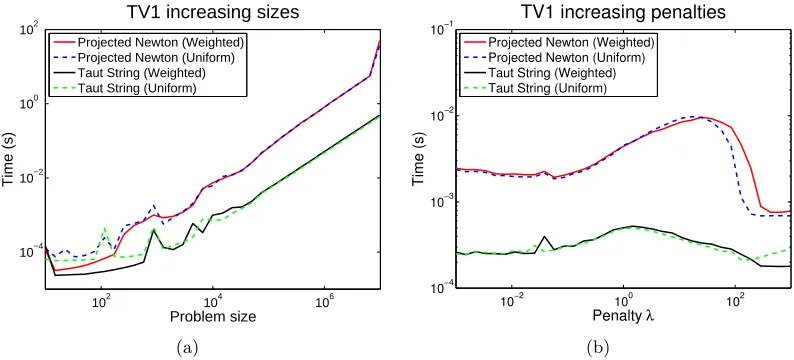
2. TV-L1: Fast Prox-Operators for Tv1D1
We begin with the 1D-TV problem (1.2) for an`1 norm choice, for which we review several
carefully tuned algorithms. Using such well–tuned algorithms pays off: we can find fast, robust, and low-memory (in fact, in place) algorithms, which are not only of independent value, but also ideal building blocks for scalably solving 2D- and higher-D TV problems.
Computation of the`1-norm TV prox-operator can be compactly written as the problem
min
x∈Rn 1
2kx−yk 2
2+λkDxk1, (2.1)
whereD is the differencing matrix, all zeros except dii=−1 anddi,i+1= 1 (1≤i≤n−1).
To solve (2.1) we will analyze an approach based on the line of “taut-string” methods.
We first introduce these methods for the unweightedTV-L1 problem (2.1), before discussing
the elementwise weighted TV problem (2.6). Most of the previous fastest methods handle only unweighted-TV. It is often nontrivial to extend them to handle weighted-TV, a problem that is crucial to several applications, e.g., segmentation (Chambolle and Darbon, 2009) and certain submodular optimization problems (Jegelka et al., 2013).
A remarkably efficient approach to TV-L1 was presented in (Condat, 2012). We will show Condat’s fast algorithm can be interpreted as a “linearized” version of the taut-string approach, a view that paves the way to obtain an equally fast solver for weighted TV-L1.
Before proceeding we note that other than (Condat, 2012), other efficient methods to
address unweighted Tv1D1 proximity have been proposed. Johnson (2013) shows how solving
Tv1Dp proximity is equivalent to computing the data likelihood of an specific Hidden Markov
Model (HMM), which suggests a dynamic programming approach based on the well-known Viterbi algorithm for HMMs. The resulting algorithm is very competitive, and guarantees
an overall O(n) performance while requiring approximately 8nstorage. Another similarly
performing algorithm was presented by Kolmogorov et al (2015) in the form of a message passing method. We will also consider these algorithms in our experimental comparison in
§5.1.
Yet another family of methods is based on projected-Netwon (PN) techniques: we also present in Appendix E a PN approach for its instructive value, and also because it provides
key subroutines for solving TV problems with p >1. Our derivation may also be helpful
similar to TV, for instance `1-trend filtering (Kim et al., 2009; Tibshirani, 2014). Indeed,
the PN approach proves to be foundational for the fast “group fused-lasso” algorithms of (Wytock et al., 2014).
2.1. The Taut-String Method for Tv1D1
While taut-string methods seem to be largely unknown in machine learning, they have been widely applied in statistics—see e.g., (Grasmair, 2007; Davies and Kovac, 2001; Barlow, 1972).
We start by transforming the problem as follows. For TV-L1, elementary manipulations, e.g., using Proposition A.4, yield the dual (re-written as a minimization problem)
min
u 1 2kD
Tuk2
2−uTDy, s.t. kuk∞≤λ. (2.2)
Without changing the minimizer, the objective (2.2) can be replaced bykDTu−yk2
2, which
then unfolds into
(u1−y1)2+
Xn−1
i=2 (−ui−1+ui−yi)
2+ (−u
n−1−yn)2.
Introducing the fixed extreme points u0 =un= 0, we can replace the problem (2.2) by
min
u Xn
i=1(−ui−1+ui−yi) 2
, s.t. kuk∞≤λ, u0 =un= 0. (2.3)
Now we perform a change of variables by defining the new set of variabless=r−u, where
ri :=Pik=1yk is the cumulative sum of input signal values. Thus, (2.3) becomes
min
s Xn
i=1(−ri−1+si−1+ri−si−yi)
2, s.t. ks−rk
∞≤λ, r0−s0=rn−sn= 0,
which upon simplification becomes
min
s Xn
i=1(si−1−si) 2
, s.t. ks−rk∞≤λ, s0= 0, sn=rn. (2.4)
Now the key trick: problem (2.4) can be shown to share the same optimum as
min
s n X
i=1 q
1 + (si−1−si)2, s.t. ks−rk∞≤λ, s0 = 0, sn=rn. (2.5)
A proof of this relationship may be found in (Steidl et al., 2005); for completeness, and also
because it will help us generalize to the weighted Tv1D1 variant, we include an alternative
proof in Appendix C.
The name “taut-string” is explained as follows. The objective in (2.5) can be interpreted
as the Euclidean length of a polyline through the points (i,si). Thus, (2.5) seeks the
minimum length polyline (the taut-string) crossing a tube of height λ with center the
cumulative sum r and having the fixed endpoints (s0, sn). An example illustrating this
0
1
2
3
4
5
6
7
8
9
10
−6
−4
−2
0
i
s
Taut−string solution
Figure 1: Example of the taut string method. The cumulative sumr of the input signal valuesy
is shown as the dashed line; the black dots mark the points (i, ri). The bottom and top of theλ-width tube are shown in red. The taut string solutionsis shown as a blue line.
Once the taut string is found, the solution for the original TV problem (2.1) can be recovered by observing that
si−si−1 = ri−ui−(ri−1−ui−1) = yi−ui+ui−1 = xi,
where we used the primal-dual relationx=y−DTu. Intuitively, the above argument shows
that the solution to the TV-L1 proximity problem is obtained as the discrete gradient of the taut string, or as the slope of its segments.
It remains to describe how to find the taut string. The most widely used approach seems to be the one due to Davies and Kovac (2001). This approach starts from the fixed point
s0 = 0, and incrementally computes the greatest convex minorant of the upper bounds on
the λ tube, as well as the smallest concave majorant of the lower bounds on the λ tube.
When both curves intersect, theleft-most point where either the majorant or the minorant
touched the tube is used to fix a first segment of the taut string. The procedure is then resumed at the end of the identified segment, and iterated until all taut string segments have been obtained. Pseudocode of this method is presented as Algorithm 1, while an example of this procedure is shown in Figure 2.
It is important to note that since we have a discrete number of points in the tube, the greatest convex minorant can be expressed as a piecewise linear function with segments of monotonically increasing slope, while the smallest concave majorant is another piecewise linear function with segments of monotonically decreasing slope. Another relevant fact is that each segment in the tube upper/lower bound enters the minorant/majorant exactly once in the algorithm, and is also removed exactly once. This limits the extent of the inner loops in the algorithm, and in fact an analysis of the computational complexity of this
behavior leads to an overall O(n) performance (Davies and Kovac, 2001).
Algorithm 1 Taut string algorithm for TV-L1-proximity 1: Inputs: input signalyof lengthn, regularizerλ.
2: Initializei= 0, concmajorant=∅,convminorant=∅,ri=P i k=1yk.
3: while i < ndo
4: Add new segment: concmajorant=concmajorant∪((i−1,ri−1−λ)→(i,ri−λ)).
5: whileconcmajorantis not concavedo
6: Merge the last two segments ofconcmajorant
7: end while
8: Add new segment: convminorant=convminorant∪((i−1,ri−1+λ)→(i,ri+λ)).
9: whileconvminorant is not convexdo
10: Merge the last two segments ofconvminorant
11: end while
12: if slope(left-most segment in concmajorant) >slope(lest-most segment in convminorant) then
13: break = left-most point where either the majorant or the minorant touched the tube 14: if break∈convminorantthen
15: Remove left-most segment of the minorant, add it to the taut-string solutionx. 16: Majorant is recalculated as a straight line frombreak to its last point.
17: end if
18: if break∈concmajorantthen
19: Remove left-most segment of the majorant, add it to the taut-string solutionx. 20: Minorant is recalculated as a straight line frombreak to its last point.
21: end if
22: end if 23: i+ + 24: end while
25: Add last segment from either the majorant or minorant to the solution x.
his proposed method. To this observation we make two claims: Condat’s method can be interpreted as a linearized version of the taut-string method (see Section 2.2); and that a careful implementation of the taut-string method can be highly competitive in practice.
2.1.1. Efficient Implementation of Taut-Strings
We propose now an efficient implementation of the taut-string method. The main idea is to carefully use double-ended queues (Knuth, 1997) to store the majorant and minorant information. Therewith, all majorant/minorant operations such as appending a segment or removing segments from either the beginning or the end of the majorant can be performend in constant time. Note however that usual double-ended queue implementations use dou-bly linked lists, dynamic arrays or circular buffers: these approaches require dynamically reallocating memory chunks at some of the insert or remove operations. But in the taut-string algorithm, the maximum number of segments of the majorant/minorant is just the
size of the input signal (n), and also the number of segments to be inserted in the queue
throughout the algorithm will be n. Making use of these facts we implement a specialized
queue based on a contiguous array of fixed length n. New segments are added from the
(1)
(2)
(3)
(4)
(5)
(6)
(7)
(8)
(9)
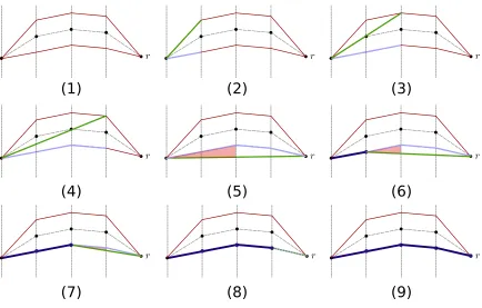
Figure 2: Example of the evolution of the taut string method. The smallest concave majorant
(blue) and largest convex minorant (green) are updated are every step. At step (1) the algorithm is initialized. Steps (2) to (4) successfully manage to update majorant and minorant without producing crossings between them. Note how while the concave majorant keeps adding segments without issue, the convex minorant must remove and merge existing segments with new ones to mantain a convex function from the origin to the new points. At step (5) the end of the tube is reached, but the minorant and majorant slopes overlap, and so it is necessary to break the segment at the left-most point where the majorant/minorant touched the tube. Since the left-most touching point is in the concave majorant it’s leftmost segment is removed and placed in the solution, while the convex minorant is updated as a straight line from the detected breakpoint to the last explored point, resulting in (6). The algorithm would then continue adding segments, but since the majorant/minorant slopes are still crossing, the procedure of fixing segments to the solution is repeated through steps (6), (7) and (8). Finally at step (9) the slopes are no longer crossing and the method would continue adding tube segments, but since the end of the tube has already been reached the algorithm stops.
requires a single memory allocation at the beginning of the algorithm, keeping the rest of queue operations free from memory management and all but the simplest pointer or index algebra.
We also store for each segment the following values: x length of the segment, y length
other calculation and code optimization details produces our implementation; these can be
reviewed in the code itself athttps://github.com/albarji/proxTV.
2.2. Linearized Taut-String Method for Tv1D1
We now present a variant, linearized version of the taut-string method. Surprisingly, the resulting algorithm turns out to be equivalent to the fast algorithm of Condat (2012), though now with a clearer interpretation based on taut-strings.
The key idea is to build linear approximations to the greatest convex minorant and smallest concave majorant, producing exactly the same results but significantly reducing the bookkeeping of the method to a handful of simple variables. We therefore replace the
greatest convex minorant and smallest convex majorant by a greatest affine minorant and
smallest affine majorant.
An example of the method is presented in Figure 3. A proof showing that this lineariza-tion does not change the resultant taut-string is given in Appendix D. In what follows, we describe the linearized method in depth.
Details. Linearized taut-string requires only the following bookkeeping variables:
1. i0: index of the current segment start
2. ¯δ: slope of the majorant
3.
¯δ: slope of the minorant
4. ¯h: height of majorant w.r.t. the λ-tube center
5. ¯
h: height of minorant w.r.t. λ-tube center
6. ¯i: index of last point where ¯δ was updated—potential majorant break point
7.
¯i: index of last point where¯δ was updated—potential minorant break point.
Figure 4 gives a geometric interpretation of these variables; we use these variables to detect minorant-majorant intersections, without the need to compute or store them explicitly.
Algorithm 2 presents full pseudocode of the linearized taut-string method. Broadly, the algorithm proceeds in the same fashion as the classic taut-string method, updating the affine approximations to the majorant and minorant at each step, and introducing a breakpoint whenever the slopes of these two functions cross.
More precisely, at each each iteration the method steps one point further through the tube, updating the minorant/majorant slopes (
¯δ, ¯δ) as well as their heights at the current
point ( ¯
h, ¯h). To check for minorant/majorant crossings it suffices to compare the slopes
(
¯δ, ¯δ), or equivalently, to check whether the height of the minorant¯h falls below the tube
bottom (since the minorant follows the tube ceiling) or the height of the majorant ¯hgrows
above the tube ceiling (since the majorant follows the tube bottom). We make use of this last variant, since updating heights turns out to be slightly cheaper than updating slopes, and so it is faster to ensure no crossing will take place before performing such updates.
(1) (2) (3)
(4) (5) (6)
(7) (8) (9)
(10) (11)
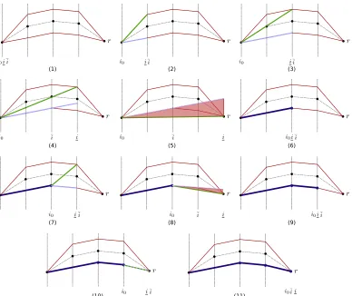
Figure 3: Example of the evolution of the linearized taut string method. The smallest affine
ma-jorant of the tube bottom (blue) and greatest affine minorant of the tube ceiling (green) are updated at every step. At step (1) the algorithm is initialized. Steps (2) to (4) suc-cessfully manage to update majorant/minorant without crossings. At step (5), however, the slopes cross, and so it is necessary to break the segment. Since the left-most tube touching point is the one in the majorant, the majorant is broken down at that point and its left-hand side is added to the solution, resulting in (6). The method is then restarted at the break point, with majorant/minorant being updated at step (7), though at step (8) once again a crossing is detected. Hence, at step (9) a breaking point is introduced again and the algorithm is restarted once more. Following this, step (10) manages to update majorant/minorant slopes up to the end of the tube, and so at step (11) the final segment is built using the (now equal) slopes.
not keep enough information to perform such an operation, so all data about minorant and majorant is discarded and the algorithm begins anew. Because of this choice the same tube
segment might be reprocessed up to O(n) times in the method, and therefore the overall
worst case performance isO(n2). This fact was already observed in (Condat, 2012).
Figure 4: Illustration of the geometric concepts involved in the linearized taut string method. The greatest linear minorant (of the tube ceiling) is depicted in green, while the smallest linear majorant (of the tube bottom) is shown in blue. Theδ slopes and hheights are presented updated up to the index shown as i.
Height variables. To implement the method described above, the height variables h
are not strictly necessary as they can be obtained from the slopes δ. However, explicitly
including them leads to efficient updating rules at each iteration, as we show below.
Suppose we are updating the heights and slopes from their estimates at step i−1 to
step i. Updating the heights is immediate given the slopes, since
hi =hi−1+δ−yi.
In other words, since we are following a line with slopeδ, the change in height from one step
to the next is given by precisely such a slope. Note, however, that in this algorithm we do
not compute absolute heights but instead relative heights with respect to theλ–tube center.
Therefore we need to account for the change in the tube center between steps i−1 and i,
which is given by ri−ri−1 =yi. This completes the update, which is shown in Algorithm
2 as lines 4 and 11.
However, it is possible that the new height h runs over or under the tube. This would
mean that we cannot continue using the current slope in the majorant or minorant, and a recalculation is needed, which again can be done efficiently by using the height information. Assume without loss of generality that the starting index of the current segment is 0 and
the absolute height of the starting point of the segment is given by α. Then, for adjusting
the minorant slope ¯δi so that it touches the tube ceiling at the current point, we note that
¯
δi =
λ+ri−α
i =
λ+ (¯hi−¯hi) +ri−α
i ,
where we have also added and subtracted the current value of ¯hi. Observe that this value was
computed using the estimateδi−1 of the slope so far, so we can rewrite it as the projection
Algorithm 2 Linearized taut string algorithm for TV-L1-proximity
1: Initializei= ¯i=
¯i= ¯h=¯h= 0,¯δ=y0+λ, ¯δ=y0−λ 2: while i < ndo
3: Find tube height: ˜λ=λifi < n−1, else ˜λ= 0
4: Update majorant height following current slope: ¯h= ¯h+ ¯δ−yi.
5: /* Check for ceiling violation: majorant is above tube ceiling */ 6: if h >¯ λ˜ then
7: Build valid segment up to last majorant breaking point: xi0+1:¯i= ¯δ. 8: Start new segment after break: (i0,
¯i) = ¯i,¯δ=yi+ 2λ, ¯δ=yi,¯h=λ, ¯h=−λ,i= ¯i+ 1
9: continue
10: end if
11: Update minorant height following current slope: ¯
h= ¯
h+ ¯δ−yi. 12: /* Check for bottom violation: minorant is below tube bottom */ 13: if
¯
h <−˜λthen
14: Build valid segment up to last minorant breaking point: xi0+1:
¯i =¯δ. 15: Start new segment after break: (i0,¯i) =
¯i,¯δ=yi, ¯δ=−2λ+yi,¯h=λ, ¯h=−λ,i=¯i+ 1
16: continue
17: end if
18: /* Check if majorant height is below the floor */ 19: if h¯≤ −˜λ then
20: Correct slope: ¯δ= ¯δ+λ˜−¯h
i−i0
21: The majorant now touches the floor: ¯h=−˜λ
22: This is a possible majorant breaking point: ¯i=i
23: end if
24: /* Check if minorant height is above the ceiling */ 25: if
¯
h≥λ˜ then
26: Correct slope:
¯δ=¯δ+ −˜λ−
¯
h i−i0
27: The minorant now touches the ceiling: ¯
h= ˜λ
28: This is a possible minorant breaking point: ¯i=i 29: end if
30: Continue building current segment: i=i+ 1 31: end while
32: Build last valid segment: xi0+1:n = ¯δ.
so for one of the added heights ¯hi produces
¯
δi=
λ+ (iδ¯i−1−ri+α)−¯hi+ri−α
i = ¯δi−1+ λ−¯hi
i ,
which generates a simple updating rule. A similar derivation holds for the minorant. The resulting updates are included in the algorithm in lines 20 and 26. After recomputing this slope we need to adjust the corresponding height back to the tube: since the heights are
relative to the tube center we can just set ¯h=λ,
¯h=−λ; this is done in lines 21 and 27.
Notice also that the special case of the last point in the tube where the taut-string
must meet sn=rn is handled by line 3, where ˜λis set to 0 at such a point to enforce this
Classic Linearized (Condat’s)
Worst-case performance O(n) O(n2)
In–memory No Yes
Other considerations Fast bookkeeping through
double-ended queues
Very fast iteration, cache
friendly
Table 1: Comparison of the main features of reviewed taut-string algorithms.
required beyond the constant number of bookkeeping variables, and in-place updates are
also possible because yi values for already fixed sections of the taut-string are not required
again, so the outputxand the input y can both refer to the same memory locations.
The resulting algorithm turns out to be equivalent, almost line by line, to the method of Condat (2012), even though its theoretical grounds are radically different: while the approach presented here has a strong geometric basis due to its taut-string relationship, (Condat, 2012) is based solely on analysis of KKT conditions. Therefore, we have shown that Condat’s fast TV method is, in fact, a linearized taut-string algorithm.
2.3. Comparison of Taut-String Methods and a Hybrid Strategy
Table 1 summarizes the main features of the classic and linearized taut-string methods reviewed so far. Although the classic taut-string method has been largely neglected in the machine learning literature, its guarantee in linear performance makes it an attractive choice. Furthermore, although we could not find any references on implementation details of this method, we have empirically seen that a very efficient solver can be produced by making use of a double-ended queue to bookkeep the majorant/minorant information.
In contrast to this, the linearized taut-string method (equivalent to Condat (2012)) features a much better performance per step in the tube traversal, mainly due to not requiring additional memory and making use of only a small constant number of variables, making the method friendly for CPU cache or registers calculation. As a tradeoff of keeping such scarce information in memory, the method does not guarantee linear performance, falling to a quadratic theoretical runtime in the worst case. This fact was already observed
in (Condat, 2012), though such worst case was deemed as pathological, claiming a O(n)
performance in all practical situations. We shall review these claims in the experimental sections in this manuscript.
The key points of Table 1 show that no taut-string variant is clearly superior. While the classic method provides a safe linear time solution to the problem, the linearized method is potentially faster but riskier in terms of worst case performance. Following these ob-servations we propose here a simple hybrid method combining both approaches: run the
linearized algorithm up to a prefixed number of steps nS, S ∈ (1,2), and if the solution
has not yet been found, we switch to the classic method. We therefore limit the worst-case
scenario toO(nS) +O(n)'O(nS), because once the classic method kicks, it will ensure an
O(n) performance guarantee.
has already run fornS steps without reaching the solution, the remaining part of the signal for which the taut-string has not yet been found is passed on to the classic method, whose solution is concatenated to the part the linearized method managed to find so far. We also report the empirical performance of this method in the experimental section.
2.4. Taut-string Methods for Weighted Tv1D1
Several applications TV require penalizing the discrete gradients individually, which can be
done by solving theweighted TV-L1 problem
minx 12kx−yk22+
Xn−1
i=1 wi|xi+1−xi|, (2.6)
where the weights{wi}ni=1−1 are all positive. To solve (2.6) using a taut-string approach, we
again begin with its dual (written as a minimization problem)
minu 12kDTuk22−uTDy s.t. |ui| ≤wi, 1≤i < n. (2.7)
Then, we repeat the derivation of the unweighted taut-string method but with a few key
modifications. More precisely, we transform (2.7) by introducing u0 =un= 0 to obtain
min
u Xn
i=1(yi−ui+ui−1)
2 s.t. |u
i| ≤wi, 1≤i < n.
Then, we perform the change of variabless=r−u, whereri:=Pik=1yk, and consider
min
s Xn
i=1(si−si−1) 2
s.t.|si−ri| ≤wi, 1≤i < n s0 = 0, sn=rn.
Finally, applying Theorem C.1 we obtain the equivalent weighted taut-string problem
min
s Xn
i=1 q
1 + (si−si−1)2 s.t.|si−ri| ≤wi, 1≤i < n, s0 = 0, sn=rn. (2.8)
Problem (2.8) differs from its unweighted counterpart (2.5) in the constraints |si−ri| ≤
wi (1≤i < n), which allow different weights for each component instead of using the same
value λ. Our geometric intuition also carries over to the weighted problem, albeit with a
slight modification: the tube we are trying to traverse now has varying widths at each step
instead of the previous fixed λwidth—Figure 5 illustrates this idea.
As a consequence of the above derivation and intuition, taut-string methods can be
produced to solve the weighted Tv1D1 problem. The original formulation of the classic
taut-string method in (Davies and Kovac, 2001) defines the limits of the tube through possibly
varying bottom and ceiling values (li, ui) ∀i, and so this method easily extends to solve
the weighted TV problem by assigning li = ri−wi, ui = ri +wi. In our pseudocode in
Algorithm 1 we just need to replaceλby the appropriate wi values.
Similar considerations apply for the linearized version (Algorithm 2), in particular, when checking ceiling/floor violations as well as when checking slope recomputations and restarts, we must account for varying tube heights. Algorithm 3 presents the precise modifications that we must make to Algorithm 2 to handle weights. Regarding the convergence of this method, the proof of equivalence with the classic taut-string method still holds in the weighted case (see Appendix D).
0
1
2
3
4
5
6
7
8
9
10
0
2
4
6
i
s
Taut−string solution
Figure 5: Example of the weighted taut string method withw= (1.35, 3.03, 0.73, 0.06, 0.71, 0.20,
0.12, 1.49, 1.41). The cumulative sum r of the input signal values y is shown as the dashed line, with the black dots marking the points (i,ri). The bottom and ceiling of
the tube are shown in red, which vary in width at each step following the weightswi.
The weighted taut string solutionsis shown as a blue line.
Algorithm 3 Modified lines for weighted version of Algorithm 2
3: Find tube height: ˜λ=wi+1 ifi < n−1, else ˜λ= 0 8: Start new segment after break: (i0,
¯i) = ¯i,¯δ=yi+wi−1+wi, ¯δ=yi+wi−1−wi, ¯h=wi, ¯
h=−wi,i= ¯i+ 1
15: Start new segment after break: (i0,¯i) =
¯i,¯δ=yi+wi−1−wi, ¯δ=yi+wi−1+wi, ¯h=wi, ¯
h=−wi,i= ¯i+ 1
3. Other One-Dimensional TV Variants
While more infrequent, replacing the`1 norm of the standard TV regularizer by an`p-norm
version can also be useful. In this section we focus first on a specialized solver for p = 2,
before discussing a less efficient but more general solver for any `p with p ≥ 1. We also
briefly cover thep=∞ case.
3.1. TV-L2: Proximity for Tv1D2
For TV-L2 proximity (p= 2) the dual to the prox-operator for (1.2) reduces to
minu φ(u) := 12kDTuk22−uTDy, s.t. kuk2 ≤λ. (3.1)
Problem (3.1) is nothing but a version of the well-known trust-region subproblem (TRS), for which a variety of numerical approaches are known (Conn et al., 2000).
We derive a specialized algorithm based on the classic Mor´e-Sorensen Newton (MSN)
method of (Mor´e and Sorensen, 1983). This method in general can be quite expensive, but
for (3.1) the Hessian is tridiagonal which can be well-exploited (see Appendix E). Curiously,
(GP) can be competitive. But for overall best performance, a hybrid MSN-GP approach is preferable.
Towards solving (3.1), consider its KKT conditions:
(DDT +αI)u=Dy,
α(kuk2−λ) = 0, α≥0, (3.2)
whereαis a Lagrange multiplier. There are two possible cases: eitherkuk2< λorkuk2 =λ.
If kuk2 < λ, then the KKT condition α(kuk2−λ) = 0, implies that α = 0 must hold
and u can be obtained immediately by solving the linear system DDTu=Dy. This can
be done inO(n) time owing to the bidiagonal structure of D. Conversely, if the solution to
DDTu=Dy lies in the interior of the ball kuk2 ≤λ, then it solves (3.2). Therefore, this
case is trivial, and we need to consider only the harder case kuk2 =λ.
For any givenα one can obtain the corresponding vectoruasuα= (DDT+αI)−1Dy.
Therefore, optimizing for ureduces to the problem of finding the “true” value of α.
An obvious approach is to solvekuαk22 =λ2. Less obvious is the MSN equation
hα:=λ−1− kuαk−12 = 0, (3.3)
which has the benefit of being almost linear in the search interval, which results in fast
convergence (Mor´e and Sorensen, 1983). Thus, the task is to find the root of the function
hα, for which we use Newton’s method, which in this case leads to the iteration
α←α−hα/h0α. (3.4)
Some calculation shows that the derivativeh0 can be computed as
1
h0α =
kuαk32
uT
α(DDT +αI)−1uα
. (3.5)
The key idea in MSN is to eliminate the matrix inverse in (3.5) by using the Cholesky
decomposition DDT +αI =RTαRα and defining a vectorqα = (RTα)−1u, so thatkqαk22=
uTα(DDT +αI)−1uα. As a result, the Newton iteration (3.4) becomes
α− hα
h0 α
= α−(kuαk−12 −λ−1)·
kuαk32
uT
α(DDT +αI)−1uα
,
= α− kuαk
2
2−λ−1kuαk32
kqαk22
,
= α− kuαk
2 2
kqαk22
1−kuαk2
λ
,
and therefore
α ← α−kuαk
2 2
kqαk22
1−kuαk2
λ
. (3.6)
As shown for TV-L1 (Appendix E), the tridiagonal structure of (DDT+αI) allows one
Algorithm 4 MSN based TV-L2 proximity
Initialize: α= 0, uα = 0.
while kuαk22−λ
> λ orgap(uα) > gap do
Compute Cholesky decomp. DDT +αI =RTαRα.
Obtainuα by solving RTαRαuα =Dy.
Obtainqα by solvingRTαqα=uα.
α=α− kuαk22
kqαk22
1− kuαk2
λ
.
end while return uα
Algorithm 5 GP algorithm for TV-L2 proximity
Initialize u0∈RN,t= 0.
while (¬ converged)do
Gradient update: vt=ut−1
4∇f(u t).
Projection: ut+1= max(1−λ/kvtk2,0)·vt.
t←t+ 1.
end while return ut.
The above ideas are presented as pseudocode in Algorithm 4. As a stopping criterion
two conditions are checked: whether the duality gap is small enough, and whetheruis close
enough to the boundary. This latter check is useful because intermediate solutions could be dual-infeasible, thus making the duality gap an inadequate optimality measure on its own.
In practice we use tolerance valuesλ = 10−6 and gap= 10−5.
Even though Algorithm 4 requires only linear time per iteration, it is fairly sophisticated, and in fact a much simpler method can be devised. This is illustrated here by a
gradient-projection method with afixed stepsizeα0, whose iteration is
ut+1 =Pk·k2≤λ(u
t−α
0∇φ(ut)). (3.7)
The theoretically ideal choice for the stepsizeα0 is given by the inverse of the Lipschitz
constant L of the gradient ∇φ(u) (Nesterov, 2007; Beck and Teboulle, 2009). Since φ(u)
is a convex quadratic, L is simply the largest eigenvalue of the Hessian DDT. Owing to
its special structure, the eigenvalues of the Hessian have closed-form expressions, namely
λi= 2−2 cos
iπ n+1
(for 1≤i≤n). The largest one isλn= 2−2 cos
(n−1)π
n
, which tends
to 4 asn→ ∞; thus the choice α0 = 1/4 is a good and cheap approximation. Pseudocode
showing the whole procedure is presented in Algorithm 5. Combining this with the fact that
the projectionPk·k2≤λ is also trivial to compute, the GP iteration (3.7) turns out to be very
attractive. Indeed, sometimes it can even outperform the more sophisticated MSN method,
though only for a very limited range of λ values. Therefore, in practice we recommend a
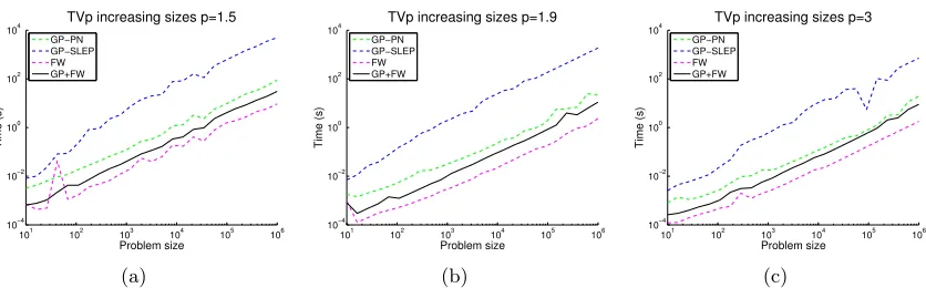
3.2. TV-Lp: Proximity for Tv1pD
For TV-Lp proximity (for 1< p <∞) the dual problem becomes
min
u φ(u) := 1 2kD
Tuk2
2−uTDy, s.t.kukq≤λ, (3.8)
where q = 1/(1−1/p). Problem (3.8) is not particularly amenable to Newton-type
ap-proaches, as neither PN (Appendix E), nor MSN-type methods (§3.1) can be applied easily.
It is partially amenable to gradient-projection (GP), for which the same update rule as
in (3.7) applies, but unlike theq = 2 case, the projection step here is much more involved.
Thus, to complement GP, we may favor the projection-free Frank-Wolfe (FW) method. As expected, the overall best performing approach is actually a hybrid of GP and FW. We summarize both choices below.
3.2.1. Efficient Projection onto the `q-ball
The problem of projecting onto the `q-norm ball is
minw d(w) := 12kw−uk22, s.t. kwkq ≤λ. (3.9)
For this problem, it turns out to be more convenient to address its Fenchel dual
minw d∗(w) := 12kw−uk22+λkwkp, (3.10)
which is actually nothing but proxλk·kp(u). The optimal solution, say w∗, to (3.9) can be
obtained by solving (3.10), by using the Moreau-decomposition (A.6) which yields
w∗ =u−proxλk·kp(u).
Projection (3.9) is computed many times within GP, so it is crucial to solve it rapidly and accurately. To this end, we first turn (3.10) into a differentiable problem and then derive a projected-Newton method following our approach presented in Appendix E.
Assume therefore, without loss of generality that u≥0, so that w≥0 also holds (the
signs can be restored after solving this problem). Thus, instead of (3.10), we solve
minw d∗(w) := 12kw−uk22+λ
X
iw p i
1/p
s.t. w≥0. (3.11)
The gradient ofd∗ may be compactly written as
∇d∗(w) =w−u+λkwk1−p pwp−1, (3.12)
wherewp−1 denotes elementwise exponentiation ofw. Elementary calculation yields
∂2
∂wi∂wjd ∗
(w) =δij 1 +λ(p−1) kwwikpp
−2
kwk−1p
+λ(1−p) wi
kwkp
p−1 wj kwkp
p−1
kwk−1p
=δij 1−cwˆpi−2
+cw¯iw¯j,
where c:= λ(1−p)kwk−1
p , ˆw :=w/kwkp, ¯w:= (w/kwkp)p−1, andδij is the Dirac delta.
In matrix notation, this Hessian’s diagonal plus rank-1 structure becomes apparent
To develop an efficient Newton method it is imperative to exploit this structure. It is
not hard to see that for a set of non-active variables ¯I the reduced Hessian takes the form
HI¯(w) = Diag 1−cwˆIp¯−2+cw¯I¯w¯TI¯. (3.14)
With the shorthand ∆ = Diag 1−cwˆpI¯−2
, the matrix-inversion lemma yields
HI¯−1(w) = ∆ +cw¯I¯w¯TI¯ −1
= ∆−1− ∆
−1cw¯ ¯
Iw¯TI¯∆−1
1 +cw¯T ¯ I∆
−1w¯ ¯ I
. (3.15)
Furthermore, since in PN the inverse of the reduced Hessian always operates on the reduced gradient, we can rearrange the terms in this operation for further efficiency; that is,
HI¯(w)−1∇I¯f(w) =v ∇I¯f(w)−
vw¯I¯ vw¯I¯T∇I¯f(w)
1/c+ ¯wI¯ vw¯I¯
, (3.16)
wherev := 1−cwˆIp¯−2
−1
, and denotes componentwise product.
The relevant point of the above derivations is that the Newton direction, and thus the
overall PN iteration can be computed inO(n) time, which results in a highly effective solver.
3.2.2. Frank-Wolfe Algorithm for TV-Lp Proximity
The Frank-Wolfe (FW) algorithm (see e.g., Jaggi (2013) for a recent overview), also known as the conditional gradient method (Bertsekas, 1999) solves differentiable optimization prob-lems over compact convex sets, and can be quite effective if we have access to a subroutine to solve linear problems over the constraint set.
The generic FW iteration is illustrated in Algorithm 6. FW offers an attractive strategy
for TV-Lp because both the descent-direction as well as stepsizes can be computed easily.
Specifically, to find the descent direction we need to solve
mins sT DDTu−Dy
, s.t. kskq≤λ. (3.17)
This problem can be solved by observing that maxkskq≤1sTz is attained by some vector
s proportional to z, of the form |s∗| ∝ |z|p−1. Therefore, s∗ in (3.17) is found by taking
z=DDTu−Dy, computings=−sgn(z) |z|p−1 and then rescalingsto meetkskq =λ.
Algorithm 6 Frank-Wolfe (FW)
Inputs: f, compact convex set D.
Initialize x0 ∈ D,t= 0.
while stopping criteria not met do
Find descent direction: minss· ∇f(xt) s.t.s∈ D.
Determine stepsize: minγf(xt+γ(s−xt)) s.t.γ ∈[0,1].
Update: xt+1=xt+γ(s−xt)
t←t+ 1.
The stepsize can also be computed in closed form owing to the objective function being
quadratic. Note the update in FW takes the formu+γ(s−u), which can be rewritten as
u+γdwithd=s−u. Using this notation the optimal stepsize is obtained by solving
minγ∈[0,1]12kD
T(u+γd)k2
2−(u+γd) T
Dy.
A brief calculation on the above problem yields
γ∗ = min{max{ˆγ,1},0},
where ˆγ =−(dTDDTu+dTDy)/(dTDDTd) is the unconstrained optimal stepsize. We
note that following (Jaggi, 2013) we also check a “surrogate duality-gap”
g(x) =xT∇f(x)−min
s∈Ds
T∇f(x) = (x−s∗)T ∇f(x),
at the end of each iteration. If this gap is smaller than the desired tolerance, the real duality gap is computed and checked; if it also meets the tolerance, the algorithm stops.
3.3. Prox Operator for TV-L∞
The final case is Tv1D∞ proximity. We mention this case only for completeness. The dual to
the prox-operator here is
minu 12kDTuk22−uTDy, s.t.kuk1≤λ. (3.18)
This problem can be again easily solved by invoking GP, where the only non-trivial step
is projection onto the `1-ball. But the latter is an extremely well-studied operation (see
e.g., Condat (2016); Liu and Ye (2009); Kiwiel (2008)), and so O(n) time routines for this
purpose are readily available. By integrating them in our GP framework an efficient prox solver is obtained.
4. Prox Operators for Multidimensional TV
We now move onto discussing how to use the efficient 1D-TV prox operators derived above within a prox-splitting framework to handle multidimensional TV (1.3) proximity.
4.1. Proximity Stacking
The basic composite objective (1.1) is a special case of the more general class of models where one may have several regularizers, so that we now solve
minx f(x) +
Xm
i=1ri(x), (4.1)
where eachri (for 1≤i≤m) is lsc and convex.
Just like the basic problem (1.1), the more complex problem (4.1) can also be tackled
via proximal methods. The key to doing so is to use inexact proximal methods along with
a technique we should call proximity stacking. Inexact proximal methods allow one to
Proximal method
+
Proximity combiner
...
Proximity operator
Proximity operator
Proximity operator Gradient
operator
Figure 6: Design schema in proximal optimization for minimizing the functionf(x) +Pm
i=1ri(x).
Proximal stacking makes the sum of regularizers appear as a single one to the proximal method, while retaining modularity in the design of each proximity step through the use of a combiner method. For non-smoothf the same schema applies by just replacing the
f gradient operator by its corresponding proximity operator.
proximity stacking allows one to compute the prox operator for the entire sum r(x) =
Pm
i=1ri(x) by “stacking” the individual ri prox operators. This stacking leads to a highly
modular design; see Figure 6 for a visualization. In other words, proximity stacking involves computing the prox operator
proxr(y) := argmin
x 1
2kx−yk 2 2+
Xm
i=1ri(x), (4.2)
by iteratively invoking the individual prox operators proxri and then combining their
out-puts. This mixing is done by means of a combiner method, which guarantees convergence
to the solution of the overall proxr(y).
Different proximal combiners can used for computing proxr (4.2). In what follows we
briefly describe some of the possibilities. The crux of all of them is that their key steps
will be proximity steps over the individual ri terms. Thus, using proximal stacking and
combination, any convex machine learning problem with multiple regularizers can be solved in a highly modular proximal framework. After this section we exemplify these ideas by applying them to two- and higher-dimensional TV proximity, which we then use within proximal solvers for addressing a wide array of applications.
4.1.1. Proximal Dykstra (PD)
The Proximal Dykstra method (Combettes and Pesquet, 2009) solves problems of the form
min
x 1
2kx−yk 2
2+r1(x) +r2(x),
which is a particular case of (4.2) form= 2. The method follows the procedure detailed in
Algorithm 7, which is guaranteed to converge to the desired solution. Using PD for proximal stacking for 2D Total-Variation was previously proposed in (Barbero and Sra, 2011).
Algorithm 7 Proximal Dykstra
Inputs: r1, r2, input signaly∈Rn.
Initialize x0 =y,p0 =q0= 0, t= 0.
while stopping criteria not met do
r2 proximity operator: zt= proxr2(xt+pt).
r2 step: pt+1 =xt+pt−zt.
r1 proximity operator: xt+1 = proxr1(zt+qt).
r1 step: qt+1 =zt+qt−xt+1.
t←t+ 1.
end while Return xt.
Algorithm 8 Parallel-Proximal Dykstra
Inputs: r1, . . . , rm, input signaly∈Rn.
Initialize x0 =y,z0i = 0, fori= 1, . . . , m;t= 0
while stopping criterion not met do
fori= 1 to m inparallel do
pi
t= proxri(z
i t) end for
xt+1 = m1 Pipit
fori= 1 to m inparallel do
zit+1 =xt+1+zti−pit end for
t←t+ 1
end while Return xt
effectiveness varies depending on the relative orientation of such polytopes. A more efficient method based on reflections instead of projections is possible, as we will see below.
More generally, if more than two regularizers are present (i.e., m >2), then it is more
fitting to use Parallel-Proximal Dykstra (PPD) (Combettes, 2009) (see Alg. 8), a
gener-alization obtained via the “product-space trick” of Pierra (1984). This parallel proximal method is attractive because it not only combines an arbitrary number of regularizers, but also allows parallelizing the calls to the individual prox operators. This feature allows us to
develop a highly parallel implementation for multidimensional TV proximity (§4.3).
4.1.2. Alternating Reflections – Douglas-Rachford (DR)
The Douglas-Rachford (DR) method was originally devised for minimizing the sum of two (nonsmooth) convex functions (Combettes and Pesquet, 2009), in the form:
min
such that (ri domf1) ∩(ri domf2) 6= ∅. The method operates by iterating a series of
reflections, and in its simplest form can be written as
zk+1= 12[Rf1Rf2 +I]zk, (4.4)
where the reflection operator Rφ := 2 proxφ−I. This method is not cleanly applicable to
problem (4.2) because of the squared norm term. Nevertheless in (Jegelka et al., 2013) a suitable transformation was proposed by making use of arguments from submodular opti-mization; a minimal background on this topic is given in Appendix A. We summarize the key ideas from (Jegelka et al., 2013) below.
Assumem= 2 andr1, r2 being Lov´asz extensions to some submodular functions
(Total-Variation is the Lov´asz extension of a submodular graph-cut problem, see Bach (2013)).
Defining ˆr1(x) = r1(x)−xTy, ˆr1 is also a Lov´asz extension of some submodular function
(see Appendix A). Therefore, we may consider the problem
proxr(y) := argmin
x 1 2kxk
2
2+ ˆr1(x) +r2(x),
which can be rewritten (using Proposition A.11) as
min
a,b ka−bk2, s.t. a∈ −Bˆr1, b∈Br2, (4.5)
where Br denotes the base polytope of submodular function corresponding to r (see
Ap-pendix A). The original solution can be recovered through x = a−b. Problem (4.5) is
still not in a form amenable to DR (4.3)—nevertheless, if we apply DR to the indicator
functions of the sets−Bˆr1, Br2, that is, to the problem
min
x δ−Brˆ1(x) +δBr2(x),
it can be shown (Bauschke, 2004) that the sequence (4.4) generated by DR is divergent, but that after a correction through projection converges to the desired solution of (4.5). Such solution is given by the pair
b= ΠBr2(zk), a= Π−Bˆr1(b). (4.6)
Although in this derivation many concepts have been introduced, suprisingly all the oper-ations in the algorithm can be reduced to performing proximity steps. Note first that the projections onto a base polytope required to get a solution (4.6) can be written in terms of proximity operators (Proposition A.12), which in this case implies
ΠBr2(z) =z−proxr2(z),
Π−Brˆ1(z) =z+ proxrˆ2(−z) =z+ proxr2(−z+y),
where we use the fact that forf(x) =φ(x) +uTx, proxf(x) = proxφ(x−u). The reflection
operations in which the DR iteration is based (4.4) can also be written in terms of proximity
steps, as we are applying DR to the indicator functions δ−Brˆ1, δBr2, and proximity for an
indicator function equals projection.
Algorithm 9 Alternating reflections – Douglas Rachford (DR)
Inputs: r1, r2 Lov´asz extensions of some submodular function, input signal y∈Rn.
Initialize z0 ∈Rn,t= 0.
Define the following operations: Π−Brˆ1(z)
def
= z+ proxr1(−z+y).
ΠBr2(z) def
= z−proxr2(z).
R−Bˆr1(z) def
= 2Π−Bˆr1(z)−z.
RBr2(z)
def
= 2ΠBr2(z)−z.
while stopping criteria not met do
zt+1= 12 h
R−Bˆr1RBr2 +I i
zk
t←t+ 1.
end while
b= ΠBr2(zt), a= Π−Bˆr1(b). Return x∗ =a−b.
4.1.3. Alternating-Direction Method of Multipliers (ADMM)
Although many times presented as a particular algorithm for solving problems involving
the minimization of a certain objetive f(x) +g(Lx) with L a linear operator (Combettes
and Pesquet, 2009), the Alternating-Direction Method of Multipliers can be thought as a general splitting strategy for solving the unconstrained minimization of a sum of functions.
This strategy boils down to transforming a problem in the form minxPmi=1fi(x) into a
saddle-point problem by introducing consensus constraints and incorporating them into the objective through augmented Lagrange multipliers,
min
x m X
i=1
fi(x) = min x,z1,...,zm
m X
i=1
fi(zi) s.t.z1 =x, . . . ,zm =x,
≡ min
x,z1,...,zm
max
u1,...,um m X
i=1
fi(zi) +uTi (zi−x) +
ρ
2kzi−xk2
.
The method then proceeds to solve this problem by alternating steps of minimization onx,
minimization on everyzi, and a gradient step on everyui.
In (Yang et al., 2013) a proposal using this method was presented to solvem–dimensional
anisotropic TV (1.3). This approach applies equally to the more general proximal stacking framework under discussion here (4.2), by the transformation
proxr(y) := argmin
x 1
2kx−yk 2 2+
Xm
i=1ri(x),
≡ min
x,z1,...,zm
max
u1,...,um 1
2kx−yk 2 2+ m X i=1
fi(zi) +uTi (zi−x) +
ρ
2kzi−xk2
.
The steps for obtaining a solution then follow as Algorithm 10. Similar to Parallel Proximal
Algorithm 10Alternating Direction Method of Multipliers (ADMM)
Inputs: r1, . . . , rm, input signaly∈Rn.
Initialize x0 =z0i =y fori= 1, . . . , m;t= 0
while stopping criterion not met do
xt+1 = y+
Pm
i=1(uit+ρzit) 1+mρ .
fori= 1 to m inparallel do
zit= proxλ
ρri(− 1 ρu
i
t+xt+1)
uit+1 =ut+1+ρ(zit+1−xt+1) end for
t←t+ 1
end while Return xt
4.1.4. Dual Proximity Methods
Another family of approaches to solve (4.2) is to compute the global proximity operator
using the Fenchel duals proxr∗
i. This can be advantageous in settings where the dual
prox-operator is easier to compute than the primal prox-operator; isotropic Total-Variation problems are an instance of such a setting, and thus investigating this approach for their anisotropic variants is worthwhile.
Indeed, in the context of image processing a popular splitting approach is given by Cham-bolle and Pock (2011), which consider a problem in the form
min
x F(Kx) +G(x),
forK some linear operator,F, G convex lower-semicontinuous functions. Through a
strat-egy similar to ADMM an equivalent saddle point problem can be obtained,
min
x maxy (Kx)
Ty+G(x)−F∗(y),
with F∗ convex conjugate ofF. This problem is then solved by alternating maximization
on yand minimization on xthrough proximity steps, as
yt+1= proxσF∗(yt+σKx¯t)
xt+1= proxτ G(xt−τK∗yt+1)
¯
xt+1=xt+1+θ(xt+1−xt),
where K∗ is the conjugate transpose of K. σ, τ and θ are algorithm parameters that
should be either selected under some bounds (Chambolle and Pock, 2011, Algorithm 1) or
readjusted every iteration making use of Lipschitz convexity of G (Chambolle and Pock,
2011, Algorithm 2), resulting in an accelerating scheme much in the style of FISTA (Beck and Teboulle, 2009). The overall procedure can also be shown to be an instance of pre-conditioned ADMM, where the preconditioning is given by the application of a proximity
step for the maximization ofy (instead of the usal dual gradient step of ADMM) and the
auxiliary point ¯x. Note also how proximity is computed over the dual F∗ instead of the
Now, this decomposition strategy can be applied for some instances of proximal
stack-ing (4.2) when the ri terms allow the particular composition
m X
i=1
ri(x) =F K1 .. . Km x
=F(Kx),
which does not hold in general but holds for 2D TV (1.4) when taking the identities
F(x) =kxk1, G(x) = 12kx−yk22,
K=
I⊗D D⊗I
,
withD the differencing matrix as before,⊗denotes Kronecker product, andxa
vectoriza-tion of the 2D input. The iterates above can then be applied easily: proximity overGis
triv-ial and proximity overF∗is also easy upon realizing that proxk·k∗
1 = proxδk·k∞≤1 = Πk·k∞≤1,
which is solved through thresholding.
A generalization of this approach is presented by Condat (2014), who considers
min
x f(x) +g(x) + m X
i=1
ri(Lix),
a problem that cleanly fits into (4.2) with f(x) = 12kx−yk2
2, g(x) = 0, L = I. The
procedure to find a solution is proposed as
¯
xt+1 = proxτ g∗ xt−τ∇f(xt)−τ
m X
i=1
L∗iuti !
xn+1 =ρx¯t+1+ (1−ρ)xt
¯
uti+1 = proxσh∗
i(u t
i+σLi(2¯xt+1−xt)) ∀i= 1, . . . , m , uti+1 =ρu¯ti+1+ (1−ρ)uti ∀i= 1, . . . , m ,
for τ, ρ parameters of the algorithm. When applying this procedure to 2D TV (m =
2, r1(x) = proximity over rows, r2(x) = proximity over columns) an algorithm almost
equivalent to Chambolle and Pock (2011) is obtained, the only difference being that here
the gradient off is used, instead of the proxG operation.
Yet another related method is the splitting approach of Kolmogorov et al (2015), which
form= 2 performs the following splitting:
min
x 1
2kx−yk 2
2+r1(x) +r2(x),
≡min
x,x0 kx−yk
2
2+r1(x) +r2(x0) s.t.x=x0,
≡min
x,x0maxz kx−yk
2
2+r1(x) +r2(x0) +zT(x−x0),
≡min
x maxz kx−yk 2
where we have made use of the Fenchel dual r2∗(z) = maxx0zTx0−r2(x0). This problem can be solved through a primal-dual minimization:
zt+1= proxσtr∗
2 z
t+σt(xt+θt(xt−xt−1))
,
xt+1= proxτt(k·−yk2 2+r1) x
t−τtzt+1
.
The primal proximity operator over the squared norm term plus r1 can be rewritten in
terms of proxr1 as
prox
τ(r1+12k·−yk22)
(w) = argmin
x
r1(x) +
1 +τ−1
2 kx−(1 +τ
−1)−1(y+τ−1w)k2 2,
= prox(1+τ−1)−1r
1 (1 +τ
−1)−1(y+τ−1w)
.
Regarding the dual step, in the previously presented methods the decompositions allowed
to disentangle the effect of a linear operator Li from each ri. The present
decomposi-tion, however, does not take into account this possibility, thus increasing the complexity of
computing r2∗. To address this difficulty the Moreau decomposition (A.3) is helpful, as
proxσr∗
2 (w) =w−σ
argmin
x
r2(x) + σ
2kx−σ
−1wk2 2
,
=w−σproxσ−1r
2(σ
−1w),
thus solving the dual proximity operator in terms of the primal proxr2. Regarding the
algo-rithm parametersθ,τ andσ, they can be adjusted at every iteration for greater performance
making use of Lipschitz convexity (Chambolle and Pock, 2014).
Lastly, and again for m = 2, both r1 and r2 can be exploited in their dual forms as
shown in Chambolle and Pock (2015) through the splitting
min
x 1
2kx−yk 2
2+r1(x) +r2(x),
≡ min
x,x1,x2
1
2kx−yk 2
2+r1(x1) +r2(x2) s.t.x=x1,x=x2
≡ min
x,x1,x2 max
z1,z2
1
2kx−yk 2
2+r1(x1) +z1T(x−x1) +r2(x2) +z2T(x−x2).
Minimizing this Lagrangian over x,x1,x2 and making use of Fenchel duals we arrive at
max
z1,z2
−12kz1+z2k22−r1∗(u1)−r2(u∗2) + (u1+u2)Ty,
which can be solved through an accelerated alternating minimization as
tk+1 =
1 +
q
1 + 4t2k
2 ,
¯
xk+1 =xk2+tk−1
tk+1
(xk2−xk2−1),
xk1+1 = proxr∗ 1(y−x¯
k 2),
xk2+1 = proxr∗
2(y−x
k+1 1 ),