An efficient distributed learning algorithm based on effective
local functional approximations
Dhruv Mahajan [email protected]
Facebook AI
Menlo Park, CA 94025, USA
Nikunj Agrawal [email protected]
Indian Institute of Technology
Dept. of Computer Science & Engineering Kanpur, India
S. Sathiya Keerthi [email protected]
Office Data Science Group Microsoft
Mountain View, CA 94043, USA
Sundararajan Sellamanickam [email protected]
Microsoft Research Bangalore, India
L´eon Bottou [email protected]
Facebook AI Research New York, NY, USA
Editor:Inderjit Dhillon
Abstract
Scalable machine learning over big data is an important problem that is receiving a lot of attention in recent years. On popular distributed environments such as Hadoop running on a cluster of commodity machines, communication costs are substantial and algorithms need to be designed suitably considering those costs. In this paper we give a novel approach to the distributed training of linear classifiers (involving smooth losses andL2regularization) that
is designed to reduce the total communication costs. At each iteration, the nodes minimize locally formed approximate objective functions; then the resulting minimizers are combined to form a descent direction to move. Our approach gives a lot of freedom in the formation of the approximate objective function as well as in the choice of methods to solve them. The method is shown to haveO(log(1/)) time convergence. The method can be viewed as an iterative parameter mixing method. A special instantiation yields a parallel stochastic gradient descent method with strong convergence. When communication times between nodes are large, our method is much faster than the Terascale method (Agarwal et al., 2011), which is a state of the art distributed solver based on the statistical query model (Chu et al., 2006) that computes function and gradient values in a distributed fashion. We also evaluate against other recent distributed methods and demonstrate superior performance of our method.
Keywords: Distributed learning, Example partitioning,L2 regularization
c
1. Introduction
In recent years, machine learning over Big Data has become an important problem, not only in web related applications, but also more commonly in other applications, e.g., in the data mining over huge amounts of user logs. The data in such applications are usually collected and stored in a decentralized fashion over a cluster of commodity machines (nodes) where communication times between nodes are significantly large. Examples of applications involving high communication costs include: Click prediction on advertisement data where the number of examples is huge and features are words which can run in to billions, and Geo distributed data across different countries/continents where cross data-center speeds are extremely slow. In such a settings, it is natural for the examples to be partitioned over the nodes.
Distributed machine learning algorithms that operate on such data are usually iterative. Each iteration involves some computation that happens locally in each node. In each iter-ation, there is also communicationof information between nodes and this is special to the distributed nature of solution. Distributed systems such as those based on the Map-Reduce framework (Dean and Ghemawat, 2008) involve additional special operations per iteration, such as the loading of data from disk to RAM. Recent frameworks such as Spark (Zaharia et al., 2010) and REEF (Weimer et al., 2015) avoid such unnecessary repeated loading of data from disk. Still, communication between nodes in each iteration is unavoidable and, its cost can be substantial when working with Big Data. Therefore, the development of effi-cient distributed machine learning algorithms that minimize communication between nodes is an important problem. The key is to come up with algorithms that minimize the number of iterations.
In this paper we consider the distributed batch training of linear classifiers in which: (a) both, the number of examples and the number of features are large; (b) the data matrix is sparse; (c) the examples are partitioned over the nodes; (d) the loss function is convex and differentiable; and, (e) theL2 regularizer is employed. This problem involves the large
scale unconstrained minimization of a convex, differentiable objective functionf(w) where w is the weight vector. The minimization is usually performed using an iterative descent method in which an iteration starts from a pointwr, computes a directiondr that satisfies
sufficient angle of descent: −gr, dr≤θ (1)
where gr = g(wr), g(w) = ∇f(w), a, b is the angle between vectors a and b, and 0 ≤
θ < π/2, and then performs a line search along the direction dr to find the next point, wr+1 = wr+tdr. Let w? = arg min
wf(w). A key side contribution of this paper is the
proof that, whenfis convex and satisfies some additional weak assumptions, the method has global linear rate of convergence (glrc)1and so it finds a pointwrsatisfyingf(wr)−f(w?)≤ inO(log(1/)) iterations. The main theme of this paper is that the flexibility offered by this method with strong convergence properties allows us to build a class of useful distributed learning methods with good computation and communication trade-off capabilities.
Take one of the most effective distributed methods, viz., SQM (Statistical Query Model) (Chu et al., 2006; Agarwal et al., 2011), which is a batch, gradient-based descent method. The gradient is computed in a distributed way with each node computing the gradient
component corresponding to its set of examples. This is followed by an aggregation of the components. We are interested in systems in which the communication time between nodes is large relative to the computation time in each node.2 For iterative algorithms such as SQM, the total training time is given by
Training time = (Tcmp+Tcom)Titer (2)
whereTcmp andTcom are respectively, the computation time and the communication time per iteration and Titer is the total number of iterations. When Tcom is large, it is not optimal to work with an algorithm such as SQM that has Tcmp small and due to which, Titer is large. In such a scenario, it is useful to ask: Q1. In each iteration, can we do more computation in each node so that the number of iterations and hence the number of communication passes are decreased, thus reducing the total computing time?
There have been some efforts in the literature to reduce the amount of communication. In one class of such methods, the current wr is first passed on to all the nodes. Then, each node p forms an approximation ˜fp of f using only its examples, followed by several
optimization iterations (local passes over its examples) to decrease ˜fp and reach a pointwp.
The wp ∀p are averaged to form the next iterate wr+1. One can stop after just one major
iteration (going from r = 0 to r = 1); such a method is referred to as parameter mixing (PM)(Mann et al., 2009). Alternatively, one can do many major iterations; such a method is referred to as iterative parameter mixing (IPM) (Hall et al., 2010). Convergence theory for such methods is inadequate (Mann et al., 2009; McDonald et al., 2010), which prompts us to ask: Q2. Is it possible to devise an IPM method that produces {wr} →w??
In another class of methods, the dual problem is solved in a distributed fashion (Pechy-ony et al., 2011; Yang, 2013; Yang et al., 2013; Jaggi et al., 2014). Let αp denote the dual
vector associated with the examples in nodep. The basic idea is to optimize{αp}in parallel
and then use a combination of the individual directions thus generated to take an overall step. In practice these methods tend to have slow convergence; see Section 4 for details.
We make a novel and simple use of the iterative descent method mentioned at the beginning of this section to design a distributed algorithm that answers Q1-Q2 positively. The main idea is to use distributed computation for generating a good search direction dr and not just for forming the gradient as in SQM. At iteration r, let us say each node p has the current iterate wr and the gradient gr. This information can be used together with the examples in the node to form a function ˆfp(·) that approximatesf(·) and satisfies
∇fˆp(wr) =gr. One simple and effective suggestion is:
ˆ
fp(w) =fp(w) + (gr− ∇fp(wr))·(w−wr) (3)
where fp is the part of f that does not depend on examples outside node p; the second
term in (3) can be viewed as an approximation of the objective function part associated with data from the other nodes. In Section 3 we give other suggestions for forming ˆfp. Now
ˆ
fp can be optimized within nodep using any method Mwhich has glrc, e.g., Trust region
method, L-BFGS, etc. There is no need to optimize ˆfp fully. We show (see Section 3) that,
in a constant number of local passes over examples in node p, an approximate minimizer
wp of ˆfp can be found such that the direction dp = wp−wr satisfies the sufficient angle
of descent condition, (1). A convex combination of the set of directions generated in the nodes, {dp} forms the overall direction dr for iteration r. Note that dr also satisfies (1).
The result is an overall distributed method that finds a pointwsatisfyingf(w)−f(w?)≤ inO(log(1/)) time. This answers Q2.
The method also reduces the number of communication passes over the examples com-pared with SQM, thus also answering Q1. The intuition here is that, if each ˆfp is a good
approximation of f, then dr will be a good global direction for minimizing f atwr, and so the method will move towardsw? much faster than SQM.
In summary, the paper makes the following contributions. First, for convex f we estab-lishglrcfor a general iterative descent method. Second, and more important, we propose a distributed learning algorithm that: (a) converges in O(log(1/)) time, thus leading to an IPM method with strong convergence; (b) is more efficient than SQM when communication costs are high; and (c) flexible in terms of the local optimization method M that can be used in the nodes.
There is also another interesting side contribution associated with our method. It is known that example-wise methods such as stochastic gradient descent (SGD) are inherently sequential and hard to parallelize (Zinkevich et al., 2010). By employing SGD as M, the local optimizer for ˜fp in our method, we obtain a parallel SGD method with good
performance as well as strong convergence properties. This contribution is covered in detail in Mahajan et al. (2013b); we give a summarized view in Subsection 3.5.
Experiments (Section 4) validate our theory as well as show the benefits of our method for large dimensional datasets where communication is the bottleneck. We give a discussion on unexplored possibilities for extending our distributed learning method in Section 5 and conclude the paper in Section 6.
2. Basic descent method
Letf ∈ C1, the class of continuously differentiable functions3,f be convex, and the gradient
g satisfy the following assumptions.
A1. g is Lipschitz continuous, i.e., ∃L >0 such thatkg(w)−g( ˜w)k ≤Lkw−w˜k ∀w,w˜.
A2. ∃ σ >0 such that (g(w)−g( ˜w))·(w−w˜)≥σkw−w˜k2 ∀w,w˜.
A1 and A2 are essentially second order conditions: iff happens to be twice continuously differentiable, thenLandσ can be viewed as upper and lower bounds on the eigenvalues of the Hessian off. A convex function f is said to beσ- strongly convex if f(w)−σ
2kwk 2 is
convex. In machine learning, all convex risk functionals in C1 having theL
2 regularization
term, λ2kwk2 areσ- strongly convex withσ=λ. It can be shown (Smola and Vishwanathan,
2008) that, if f isσ-strongly convex, thenf satisfies assumption A2.
Let fr=f(wr), gr =g(wr) andwr+1=wr+tdr. Consider the following standard line search conditions.
Armijo: fr+1 ≤fr+αgr·(wr+1−wr) (4)
Wolfe: gr+1·dr ≥βgr·dr (5)
where 0< α < β <1.
Algorithm 1:Descent method for f
Choose w0;
for r= 0,1. . .do
1. Exit ifgr= 0;
2. Choose a directiondr satisfying (1);
3. Do line search to chooset >0 so thatwr+1 =wr+tdr satisfies the Armijo-Wolfe conditions (4) and (5);
end
Let us now consider the general descent method in Algorithm 1 for minimizing f. The following result shows that the algorithm is well-posed. A proof is given in the appendix B.
Lemma 1. Supposegr·dr<0. Then{t: (4) and (5) hold forwr+1=wr+tdr}= [tβ, tα],
where 0< tβ < tα, and tβ,tα are the unique roots of
g(wr+tβdr)·dr =βgr·dr, (6)
f(wr+tαdr) =fr+tααgr·dr, tα >0. (7)
Theorem 2. Let w? = arg minwf(w) and f? = f(w?).4 Then {wr} → w?. Also, we
have glrc, i.e., ∃ δ satisfying 0 < δ < 1 such that (fr+1 −f?) ≤ δ(fr −f?) ∀ r ≥ 0, and, fr−f? ≤is reached after at most log((log(1f0−/δf?))/) iterations. An upper bound onδ is (1−2α(1−β)Lσ22cos2θ).
A proof of Theorem 2 is given in the appendix B. If one is interested only in proving convergence, it is easy to establish under the assumptions made; such theory goes back to the classical works of Wolfe (Wolfe, 1969, 1971). But proving glrc is harder. There exist proofs for special cases such as the gradient descent method (Boyd and Vandenberghe, 2004). The glrc result in Wang and Lin (2013) is only applicable to descent methods that are “close” (see equations (7) and (8) in Wang and Lin (2013)) to the gradient descent method. Though Theorem 2 is not entirely surprising, as far as we know, such a result does not exist in the literature.
Remark 1. It is important to note that the rate of convergence indicated by the upper bound on δ given in Theorem 2 is pessimistic since it is given for a very general descent algorithm that includes plain batch gradient descent which is known to have a slow rate of convergence. Therefore, it should not be misconstrued that the indicated slow convergence rate would hold for all methods falling into the class of methods covered here. Depending on the method used for choosingdr, the actual rate of convergence can be a lot better. For example, we observe very good rates for our distributed method, FADL; see the empirical results in Section 4 and also the comments made in Remark 2 of Section 3.
3. Distributed training
In this section we discuss full details of our distributed training algorithm. Let{xi, yi} be
the training set associated with a binary classification problem (yi ∈ {1,−1}). Consider a
linear classification model,y = sgn(wTx). Letl(w·xi, yi) be a continuously differentiable loss
function that has Lipschitz continuous gradient. This allows us to consider loss functions such as least squares (l(s, y) = (s−y)2), logistic loss (l(s, y) = log(1 + exp(−sy)) and squared hinge loss (l(s, y) = max{0,1−ys}2). Hinge loss is not covered by our theory since
it is non-differentiable.
Suppose the training examples are distributed inP nodes. Let: Ip be the set of indicesi
such that (xi, yi) sits in thep-th node;Lp(w) =Pi∈Ipl(w;xi, yi) be the total loss associated
with nodep; and,L(w) =P
pLp(w) be the total loss over all nodes. Our aim is to minimize
the regularized risk functionalf(w) given by
f(w) = λ 2kwk
2+L(w) = λ
2kwk
2+X
p
Lp(w), (8)
where λ > 0 is the regularization constant. It is easy to check that g = ∇f is Lipschitz continuous.
3.1. Our approach
Our distributed method is based on the descent method in Algorithm 1. We use a master-slave architecture.5 Let the examples be partitioned over P slave nodes. Distributed com-puting is used to compute the gradientgr as well as the directiondr. In ther-th iteration,
let us say that the master has the currentwr and gradientgr. One can communicate these to all P (slave) nodes. The direction dr is formed as follows. Each node p constructs an approximation off(w) using only information that is available in that node, call it ˆfp(w),
and (approximately) optimizes it (starting fromwr) to get the point wp. Letdp=wp−wr.
Then dr is chosen to be any convex combination of dp ∀p. Doing line search along the dr
direction completes ther-th iteration. Line search involves distributed computation, but it is inexpensive; we give details in Subsection 3.4.
We want to point out that ˆfp can change withr, i.e., one is allowed to use a different ˆfp
in each outer iteration. We just don’t mention it as ˆfpr to avoid clumsiness of notation. In fact, all the choices for ˆfp that we discuss below in Subsection 3.2 are such that ˆfp depends
on the current iterate,wr.
3.2. Choosing fˆp
Our method offers great flexibility in choosing ˆfp and the method used to optimize it. We
only require ˆfp to satisfy the following.
A3. fˆp is σ-strongly convex, has Lipschitz continuous gradient and satisfies gradient con-sistency at wr: ∇fˆp(wr) =gr.
Below we give several ways of forming ˆfp. The σ-strongly convex condition is easily
taken care of by making sure that theL2 regularizer is always a part of ˆfp. This condition
implies that
ˆ
fp(wp)≥fˆp(wr) +∇fˆp(wr)·(wp−wr) + σ
2kwp−w
rk2. (9)
The gradient consistency condition is motivated by the need to satisfy the angle condition (1). Sincewp is obtained by starting fromwr and optimizing ˆfp, it is reasonable to assume
that ˆfp(wp)<fˆp(wr). Using these in (9) gives−gr·dp >0. Sincedris a convex combination
of the dp it follows that−gr·dr>0. Later we will formalize this to yield (1) precisely.
A general way of choosing the approximating functional ˆfp is
ˆ fp(w) =
λ 2kwk
2+ ˜L
p(w) + ˆLp(w), (10)
where ˜Lpis an approximation ofLpand ˆLp(w) is an approximation ofL(w)−Lp(w) =Pq6=p Lq(w). A natural choice for ˜Lp is Lp itself since it uses only the examples within nodep;
but there are other possibilities too. To maintain communication efficiency, we would like to design an ˆLp such that it does not explicitly require any examples outside node p. To
satisfy A3 we need ˆLp to have Lipschitz continuous gradient. Also, to aid in satisfying
gradient consistency, appropriate linear terms are added. We now suggest five choices for ˆ
fp.
Linear Approximation. Set ˜Lp =Lpand choose ˆLpbased on the first order Taylor series.
Thus,
˜
Lp(w) =Lp(w), Lˆp(w) = (∇L(wr)− ∇Lp(wr))·(w−wr). (11)
(The zeroth order term needed to get f(wr) = ˆf(wr) is omitted everywhere because it is a constant that plays no role in the optimization.) Note that∇L(wr) =gr−λwr and so it is locally computable in node p; this comment also holds for the methods below.
Hybrid approximation. This is an improvement over the linear approximation where we add a quadratic term to ˆLp. Since the loss term in (8) is total loss (and not averaged
loss), this is done by using (P−1) copies of the quadratic term of Lp to approximate the
quadratic term ofP
q6=pLq.
˜
Lp(w) =Lp(w), (12)
ˆ
Lp(w) = (∇L(wr)− ∇Lp(wr))·(w−wr) + P −1
2 (w−w
r)THr
p(w−wr), (13)
where Hpr is the Hessian of Lp at wr. This corresponds to using subsampling to
approx-imate the Hessian of L(w)−Lp(w) at wr utilizing only the local examples. Subsampling
based Hessian approximation is known to be very effective in optimization for machine learning (Byrd et al., 2012).
Quadratic approximation. This is a pure quadratic variant where a second order ap-proximation is used for ˜Lp too.
˜
Lp(w) =∇Lp(wr)·(w−wr) +
1
2(w−w
r)THr
p(w−wr), (14)
ˆ
Lp(w) = (∇L(wr)− ∇Lp(wr))·(w−wr) + P −1
2 (w−w
r)THr
p(w−wr). (15)
Nonlinear approximation. Here the idea is to use P −1 copies of Lp to approximate
P
q6=pLq.
˜
Lp(w) =Lp(w), (16)
ˆ
Lp(w) = (∇L(wr)−P∇Lp(wr))·(w−wr) + (P−1)Lp(w). (17)
A somewhat similar approximation is used in Sharir et al. (2014). But the main algorithm where it is used does not have deterministic monotone descent like our algorithm. The gradient consistency condition, which is essential for establishing function descent, is not respected in that algorithm. In Section 4 we compare our methods against the method in Sharir et al. (2014).
BFGS approximation. For ˜Lp we can either use Lp or a second order approximation,
like in the approximations given above. For ˆLp we can use a second order term, 12(w− wr)·H(w−wr) where H is a positive semi-definite matrix; for H we can use a diagonal approximation or keep a limited history of gradients and form a BFGS approximation of L−Lp.
Remark 2. The distributed method described above is an instance of Algorithm 1 and so Theorem 2 can be used. In Theorem 2 we mentioned a convergence rate, δ. For cosθ=σ/Lthis yields the rateδ = (1−2α(1−β)(σL)4). This rate is obviously pessimistic given that it applies to general choices of ˆfp satisfying minimal assumptions. Actual rates
of convergence depend a lot on the choice made for ˆfp. Suppose we choose ˆfp via Hybrid,
Quadratic or Nonlinear approximation choices mentioned in Subsection 3.2 and minimize ˆ
fp exactly in the inner optimization. These approximations are invariant to coordinate
transformations such asw0 =Bw, where B is a positive definite matrix. Note that Armijo-Wolfe line search conditions are also unaffected by such transformations. What this means is that, at each iteration, we can, without changing the algorithm, choose for analysis a coordinate transformation that gives the best rate. The Linear approximation choice for
ˆ
fp does not enjoy this property. This explains why the Hybrid, Quadratic and Nonlinear
approximations perform so well and give great rates of convergence in practice; see the experiments in Section 4.7 and Subsection 4.9.1. Proving much better convergence rates for FADL using these approximations would be interesting future work.
In Section 4 we evaluate some of these approximations in detail.
3.3. Convergence theory
In practice, exactly minimizing ˆfp is infeasible. For convergence, it is not necessary for wp
to be the minimizer of ˆfp; we only need to find wp such that the direction dp = wp−wr
satisfies (1). The angleθ needs to be chosen right. Let us discuss this first. Let ˆw?p be the minimizer of ˆfp. It can be shown (see appendix B) that wˆ?p−wr,−gr≤cos−1 σL. To allow
forwp being an approximation of ˆw?p, we chooseθ such that
π
2 > θ >cos −1 σ
L. (18)
The following result shows that if an optimizer withglrc is used to minimize ˆfp, then, only
Lemma 3. Assumegr6= 0. Suppose we minimize ˆfpusing an optimizerMthat starts from v0 = wr and generates a sequence {vk} having glrc, i.e., ˆfp(vk+1)−fˆp? ≤ δ( ˆfp(vk)−fˆp?),
where ˆfp? = ˆfp( ˆw?p). Then, there exists ˆk (which depends only on σ and L) such that
−gr, vk−wr≤θ ∀k≥kˆ.
Lemma 3 can be combined with Theorem 2 to yield the following convergence theorem.
Theorem 4. Supposeθsatisfies (18), Mis as in Lemma 3 and, in each iterationr and for each p, ˆk or more iterations of M are applied to minimize ˆfp (starting from wr) and get wp. Then the distributed method converges to a point w satisfying f(w)−f(w?) ≤ in O(log(1/)) time.
Proofs of Lemma 3 and Theorem 4 are given in appendix B.
3.4. Practical implementation.
We refer to our method by the acronym, FADL - Function Approximation based Distributed Learning. Going with the practice in numerical optimization, we replace (1) by the condi-tion, −gr·dr >0 and use α = 10−4,β = 0.9 in (4) and (5). In actual usage, Algorithm 1 can be terminated whenkgrk ≤gkg0kis satisfied at some r. Let us take line search next.
Onw=wr+tdr, the loss has the forml(zi+tei, yi) wherezi=wr·xiandei =dr·xi. Once
we have computedzi∀iandei∀i, the distributed computation off(wr+tdr) and its
deriva-tive with respect to t is cheap as it does not involve any computation involving the data,
{xi}. Thus, manytvalues can be explored cheaply. Sincedr is determined by approximate
optimization,t= 1 is expected to give a decent starting point. We first identify an interval [t1, t2] ⊂ [tβ, tα] (see Lemma 1) by starting from t = 1 and doing forward and backward
stepping. Then we check if t1 ort2 is the minimizer of f(wr+tdr) on [t1, t2]; if not, we do
several bracketing steps in (t1, t2) to locate the minimizer approximately. Finally, when
us-ing methodM, we terminate it after a fixed number of steps, ˆk; we have found that, setting ˆ
k to match computation and communication costs works effectively. Algorithm 2 gives all the steps of FADL while also mentioning the distributed communications and computations involved.
Choices for M. There are many good methods having (deterministic) glrc: L-BFGS, TRON (Lin et al., 2008), Primal coordinate descent (Chang et al., 2008), etc. One could also use methods with glrcin the expectation sense (in which case, the convergence in Theorem 4 should be interpreted in some probabilistic sense). This nicely connects our method with recent literature on parallel SGD. We discuss this in the next subsection only briefly as it is outside the scope of the current paper. See our related work (Mahajan et al., 2013b) for details. For the experiments of this paper we do the following. For optimizing the quadratic approximation in (10) with (14)-(15), we used the conjugate-gradient method (Shewchuk, 1994). For all other (non-quadratic) approximations of FADL as well as all nonlinear solvers needed by other methods, we used TRON.
3.5. Connections with parallel SGD
For large scale learning on a single machine, example-wise methods6 such as stochastic gradient descent (SGD) and its variations (Bottou, 2010; Johnson and Zhang, 2013) and dual
Algorithm 2: FADL - Function Approximation based Distributed Learning. com:
communication; cmp: = computation; agg: aggregation. Mis the optimizer used for minimizing ˆfp.
Choose w0;
for r= 0,1. . .do
1. Computegr (com: wr;cmp: Two passes over data;agg: gr); By-product:
{zi=wr·xi};
2. Exit ifkgrk ≤gkg0k;
3. forp= 1, . . . , P (in parallel) do
4. Setv0 =wr;
5. fork= 0,1, . . . ,ˆkdo
6. Find vk+1 using one iteration ofM; end
7. Setwp=vˆk+1; end
8. Setdr as any convex combination of{wp} (agg: wp);
9. Compute{ei =dr·xi}(com: dr;cmp: One pass over data);
10. Do line search to findt(for eacht: com: t;cmp: l and∂l/∂t agg: f(wr+tdr)
and its derivative wrtt); 11. Setwr+1 =wr+tdr;
end
coordinate ascent (Hsieh et al., 2008) perform quite well. However, example-wise methods are inherently sequential. If one employs a method such as SGD as M, the local optimizer for ˜fp, the result is, in essence, a parallel SGD method. However, with parameter mixing
and iterative parameter mixing methods (Mann et al., 2009; Hall et al., 2010; McDonald et al., 2010) (we briefly discussed these methods in Section 1) that do not do line search, convergence theory is limited, even that requiring a complicated analysis (Zinkevich et al., 2010); see also Mann et al. (2009) for some limited results. Thus, the following has been an unanswered question: Q3. Can we form a parallel SGD method with strong convergence properties such as glrc?
As one special instantiation of our distributed method, we can use, for the local opti-mization methodM, any variation of SGD withglrc(in expectation), e.g., the one in John-son and Zhang (2013). For this case, in a related work of ours (Mahajan et al., 2013b) we show that our method has O(log(1/)) time convergence in a probabilistic sense. The result is a strongly convergent parallel SGD method, which answers Q3. An interesting side observation is that, the single machine version of this instantiation is very close to the variance-reducing SGD method in Johnson and Zhang (2013). We discuss this next.
Connection with SVRG. Let us take the ˆfp in (11). Let np = |Ip| be the number of
examples in nodep. Define ψi(w) =npl(w·xi, yi) +λ2kwk2. It is easy to check that
∇fˆp(w) =
1 np
X
i∈Ip
Thus, plain SGD updates applied to ˆfp has the form
w=w−η(∇ψi(w)− ∇ψi(wr) +gr), (20)
which is precisely the update in SVRG. In particular, the single node (P = 1) imple-mentation of our method using plain SGD updates for optimizing ˆfp is very close to the
SVRG method.7 While Johnson and Zhang (2013) motivate the update in terms of variance reduction, we derive it from a functional approximation viewpoint.
3.6. Computation-Communication tradeoff
In this subsection we do a rough analysis to understand the conditions under which our method (FADL) is faster than the SQM method (Chu et al., 2006; Agarwal et al., 2011) (see Section 1). This analysis is only for understanding the role of various parameters and not for getting any precise comparison of the speed of the two methods.
Compared to the SQM method, FADL does a lot more computation (optimize ˆfp) in
each node. On the other hand FADL reaches a good solution using a much smaller number of outer iterations. Clearly, FADL will be attractive for problems with high communication costs, e.g., problems with a large feature dimension. For a given distributed computing environment and specific implementation choices, it is easy to do a rough analysis to under-stand the conditions in which FADL will be more efficient than SQM. Consider a distributed grid of nodes in anAllReducetree. Let us use a common method such as TRON for imple-menting SQM as well as for Min FADL. Assuming that TSQMouter>3.0TFADLouter (where TFADLouter and TSQMouter are the number of outer iterations required by SQM and FADL), we can do a rough analysis of the costs of SQM and FADL (see appendix A for details) to show that FADL will be faster when the following condition is satisfied.
nz m <
γP
2ˆk (21)
where: nz is the number of nonzero elements in the data, i.e., {xi}; m is the feature
dimension; γ is the relative cost of communication to computation (e.g. 100−1000);P is the number of nodes; and ˆk is the number of inner iterations of FADL. Thus, the larger the dimension (m) is, and the higher the sparsity in the data is, FADL will be better than SQM.
4. Experiments
In this section, we demonstrate the effectiveness of our method by comparing it against several existing distributed training methods on five large data sets. We first discuss our experimental setup. We then briefly list each method considered and then do experiments to decide the best overall setting for each method. This applies to our method too, for which the setting is mainly decided by the choice made for the function approximation,
ˆ
fp; see Subsection 3.2 for details of these choices. Finally, we compare, in detail, all the
methods under their best settings. This study clearly demonstrates scenarios under which our method performs better than other methods.
4.1. Experimental Setup
We ran all our experiments on a Hadoop cluster with 379 nodes and 10 Gbit interconnect speed. Each node has Intel (R) Xeon (R) E5-2450L (2 processors) running at 1.8 GHz. Since iterations in traditional MapReduceare slower (because of job setup and disk access costs), as in Agarwal et al. (Agarwal et al., 2011), we build anAllReducebinary tree between the mappers8. The communication bandwidth is 1 Gbps (gigabits per sec).
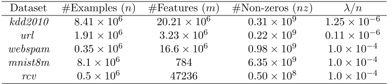
Dataset #Examples (n) #Features (m) #Non-zeros (nz) λ/n
kdd2010 8.41×10⁶ 20.21×10⁶ 0.31×10⁹ 1.25×10⁻⁶
url 1.91×10⁶ 3.23×10⁶ 0.22×10⁹ 0.11×10⁻⁶
webspam 0.35×10⁶ 16.6×10⁶ 0.98×10⁹ 1.0×10⁻⁴
mnist8m 8.1×10⁶ 784 6.35×10⁹ 1.0×10⁻⁴
rcv 0.5×10⁶ 47236 0.50×10⁸ 1.0×10⁻⁴
Table 1: Properties of datasets.
Data Sets. We consider the following publicly available datasets having a large number of examples:9 kdd2010, url, webspam, mnist8m and rcv. Table 1 shows the numbers of examples, features, nonzero in data matrix and the values of regularizer λ used. The regularizer for each dataset is chosen to be the optimal value that gives the best performance on a small validation set. We use these datasets mainly to illustrate the validity of theory, and its utility to distributed machine learning. In real scenarios of Big data, the datasets are typically much larger. Note thatkdd2010,urland webspamare large dimensional (mis large) while mnist8m and rcv are low/medium dimensional (m is not high). This division of the datasets is useful because communication cost in example-partitioned distributed methods is mainly dependent onm (see Appendix A) and so these datasets somewhat help to see the effect of communications cost.
We use thesquared-hinge lossfunction for all the experiments. Unless stated differently, for all numerical optimizations we use the Trust Region Newton method (TRON) proposed in Lin et al. (2008).
Evaluation Criteria. We use the relative difference to the optimal function value and the Area under Precision-Recall Curve (AUPRC) (Sonnenburg and Franc, 2010; Agarwal et al., 2013)10 as the evaluation criteria. The former is calculated as (f −f∗)/f∗ in log scale, wheref∗is the optimal function value obtained by running theTERAalgorithm (see below) for a very large number of iterations.
4.2. Methods for comparison
We compare the following methods.
8. Note that we do not use the pipelined version and hence we incur an extra multiplicativelogP cost in communication.
9. These datasets are available at: http://www.csie.ntu.edu.tw/~cjlin/libsvmtools/datasets/. For
mnist8mwe solve the binary problem of separating class “3” from others.
• TERA:The Terascale method (TERA) (Agarwal et al., 2011) is the best representative method from the SQM class (Chu et al., 2006). It can be considered as the state-of-the-art distributed solver and therefore an important baseline.
• ADMM: We use the example partitioning formulation of the Alternating Direction Method of Multipliers (ADMM) (Boyd et al., 2011; Zhang et al., 2012). ADMM is a dual method which is very different from our primal method; however, like our method, it solves approximate problems in the nodes and iteratively reaches the full batch solution.
• CoCoA: This method (Jaggi et al., 2014) represents the class of distributed dual methods (Pechyony et al., 2011; Yang, 2013; Yang et al., 2013; Jaggi et al., 2014) that, in each outer iteration, solve (in parallel) several local dual optimization problems.
• DANE: This is the Newton based method described in Sharir et al. (2014) that uses a function approximation similar to FADL.
• DiSCO:This (Zhang and Xiao, 2015) is a distributed Newton method designed with communication-efficiency in mind.
• Our method (FADL): This is our method described in detail in Section 3 and more specifically, in Algorithm 2.
4.3. Study of TERA
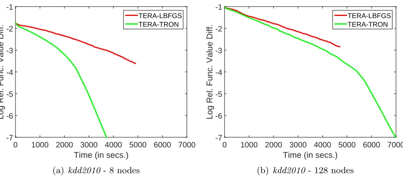
A key attractive property of TERA is that the number of outer iterations pretty much remains constant with respect to the number of distributed nodes used. As recommended by Agarwal et al. (2011), we find a local weight vector per node by minimizing the local objective function (based only on the examples in that node) using five epochs of SGD (Bot-tou, 2010). (The optimal step size is chosen by running SGD on a subset of data.) We then average the weights from all the nodes (on a per-feature basis as explained in Agarwal et al. (2011)) and use the averaged weight vector to warm start TERA.11 Agarwal et al. (2011) use the LBFGS method as the trainer whereas we use TRON. To make sure that this does not lead to bias, we try both, TERA-LBFGS and TERA-TRON. Figure 1 compares the progress of objective function for these two choices. Clearly, TERA-TRON is superior. We observe similar behavior on the other datasets also. Given this, we restrict ourselves to TERA-TRON and simply refer to it as TERA.
4.4. Study of ADMM
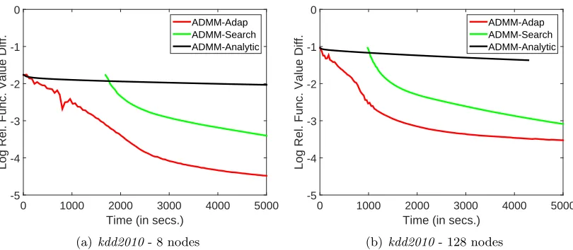
The ADMM objective function (Boyd et al., 2011) has a quadratic proximal term called augmented Lagrangian with a penalty parameter ρ multiplying it. In general, the perfor-mance of ADMM is very sensitive to the value of ρ and hence making a good choice for it is crucial. We consider three methods for choosing ρ.
Time (in secs.)
0 1000 2000 3000 4000 5000 6000 7000
Log Rel. Func. Value Diff.
-7 -6 -5 -4 -3 -2 -1
TERA-LBFGS TERA-TRON
(a)kdd2010- 8 nodes
Time (in secs.)
0 1000 2000 3000 4000 5000 6000 7000
Log Rel. Func. Value Diff.
-7 -6 -5 -4 -3 -2 -1
TERA-LBFGS TERA-TRON
(b)kdd2010- 128 nodes
Figure 1: Plots showing the time efficiency of TERA methods forkdd2010.
Even though there is no supporting theory, Boyd et al (Boyd et al., 2011) suggest an approach by which ρ is adapted in each iteration; see Equation (3.13) in Section 3.4.1 of that paper. We will refer to this choice asAdap.
Recently, Deng and Yin (2012) proved a linear rate of convergence for ADMM under assumptions A1 and A2 (see Section 2) on ADMM functions. As a result, their analysis also hold for the objective function in (8). They also give an analytical formula to setρ in order to get the best theoretical linear rate constant. We will refer to this choice of ρ as
Analytic.
We also consider a third choice, ADMM-Search in which, we start with the value of ρ given by Analytic, choose several values of ρ in its neighborhood and select the best ρ by running ADMM for 10 iterations and looking at the objective function value. Note that this step takes additional time and causes a late start of ADMM.
Figure 2 compares the progress of the training objective function for the three choices on kdd2010 for P = 8 and P = 128. Analytic is an order of magnitude slower than the other two choices. Search works well. However, a significant amount of initial time is spent on finding a good value forρ, thus making the overall approach slow. Adapcomes out to be the best performer among the three choices. Similar observations hold for other datasets and other choices ofP. So, for ADMM, we will fixAdap as the way of choosingρand refer to ADMM-Adap simply as ADMM.
Time (in secs.)
0 1000 2000 3000 4000 5000
Log Rel. Func. Value Diff.
-5 -4 -3 -2 -1 0
ADMM-Adap ADMM-Search ADMM-Analytic
(a)kdd2010- 8 nodes
Time (in secs.)
0 1000 2000 3000 4000 5000
Log Rel. Func. Value Diff.
-5 -4 -3 -2 -1 0
ADMM-Adap ADMM-Search ADMM-Analytic
(b)kdd2010- 128 nodes
Figure 2: Plots showing the time efficiency of ADMM methods for kdd2010.
4.5. Study of CoCoA
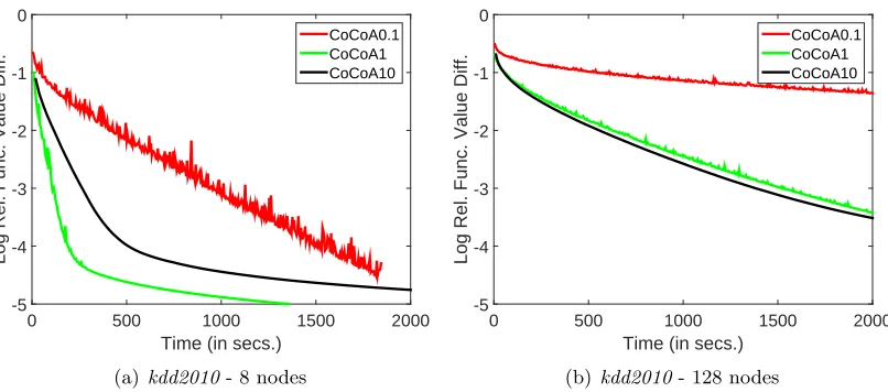
In CoCoA (Jaggi et al., 2014) the key parameter is the approximation level of the inner iterations used to solve each projected dual sub-problem. The number of epochs of coor-dinate dual ascent inner iterations plays a crucial role. We try the following choices for it: 0.1, 1 and 10.12 Figure 3 compares the progress of the objective function on kdd2010 for two choices of nodes, P = 8 and P = 128. We find the choice of 1 epoch to work well reasonably consistently over all the five datasets and varying number of nodes. So we fix this choice and refer to the resulting method simply as CoCoA. Note in Figure 3 that the (primal) objective function does not decrease continuously with time. This is because it is a dual method and so monotone descent of the objective function is not assured.13
4.6. Study of DANE
In our detailed comparison study later in this section, we will also include another method called DANE, which has some resemblance to FADL. This is the Newton based method described in Sharir et al. (2014). Even though this method is very different in spirit from our method, it uses a function approximation similar to our Nonlinear approximation idea; we briefly discussed this in Subsection 3.2. DANE is a non-monotone method that is based on fixed step sizes, with a probabilistic convergence theory to support it.
DANE has two parameters, µand η in the function approximation; µis the coefficient for the proximal term and η is used for defining the direction. Sharir et al. (2014) do not prove convergence for any possible choices ofµandηvalues; their practical recommendation is to useµ= 3λandη= 1. The choice ofµin particular, turns out to be quite sub-optimal. We found that there was no single value ofµ that is good for all datasets, and so it needs to be tuned for each dataset. So, to improve DANE, we included an initial µ-tuning step.
12. The examples were randomly shuffled for presentation. When the number of epochs is a fraction, e.g., 0.1, the inner iteration was stopped after 10% of the examples were presented.
Time (in secs.)
0 500 1000 1500 2000
Log Rel. Func. Value Diff.
-5 -4 -3 -2 -1 0
CoCoA0.1 CoCoA1 CoCoA10
(a)kdd2010- 8 nodes
Time (in secs.)
0 500 1000 1500 2000
Log Rel. Func. Value Diff.
-5 -4 -3 -2 -1 0
CoCoA0.1 CoCoA1 CoCoA10
(b)kdd2010- 128 nodes
Figure 3: Plots showing the time efficiency of CoCoA settings for kdd2010.
We start withµ= 3∗λand use an initial set of four outer iterations to choose theµvalue that gives the best improvement in objective function. Starting from µ = 3∗λ we try several values ofµ in the direction of µ change that leads to improvement. After the first four outer iterations, we fix µat the chosen best value for the remaining iterations. (Note that the cost associated with tuningµhas to be included in the overall cost of DANE.) As we will see later in Subsection 4.9, in spite of all this tuning, DANE did not converge in several situations. Essentially, the issue is that µhas to be adaptive - DANE needs to use different choices of µ in the early, middle and end stages of one training. But then, this is nearly akin to doing a kind of line search in each outer iteration. As opposed to DANE, note that FADL is a monotone method directly based on line search, and it does not need the proximal term to restrict step-sizes. Also, unlike DANE, all the parameters of FADL are fixed to default values for all datasets.
The choice of inner optimizer for DANE is crucial for its efficiency. We tried SVRG (Johnson and Zhang, 2013) and also TRON (Lin et al., 2008). Both did well, but SVRG was better, especially for small number of nodes. So we did a more detailed study of SVRG. We tried two choices. (a) Fix the number of epochs for the local (inner) optimization to some good value, e.g., 10. (b) Always choose the number of epochs for the local (inner) optimization to be such that the cost of local computation in a node is matched with the communications cost. Choice (b) gave a better solution. So we have used it for DANE.
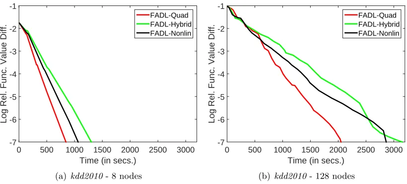
4.7. Study of FADL
Recall from Subsection 3.2 the various choices that we suggested for ˆfp. We are yet to
Time (in secs.)
0 500 1000 1500 2000 2500 3000
Log Rel. Func. Value Diff.
-7 -6 -5 -4 -3 -2 -1
FADL-Quad FADL-Hybrid FADL-Nonlin
(a)kdd2010- 8 nodes
Time (in secs.)
0 500 1000 1500 2000 2500 3000
Log Rel. Func. Value Diff.
-7 -6 -5 -4 -3 -2 -1
FADL-Quad FADL-Hybrid FADL-Nonlin
(b) kdd2010- 128 nodes
Figure 4: Plots showing the time efficiency of the three function approximations of FADL forkdd2010.
Figure 4 compares the progress of the training objective function for various choices of ˆfp. Among the choices, the quadratic approximation for ˆfp gives the best performance,
although the Hybrid and Nonlinear approximations also do quite well. We observe this reasonably consistently in other datasets too. Hence, from the set of methods considered in this subsection we choose FADL-Quadratic approximation as the only method for further analysis, and simply refer to this method as FADL hereafter.
Why does the quadratic approximation do better than hybrid and nonlinear approxi-mations? We do not have a precise answer to this question, but we give some arguments in support. In each outer iteration, the function approximation idea is mainly used to get a good direction. Recall from Subsection 3.2 that different choices use different approxima-tions for ˜Lp and ˆLp. Using the same “type” (meaning linear, nonlinear or quadratic) for
both, ˜Lp and ˆLp is possibly better for direction finding. Second, the direction finding could
be more sensitive to the nonlinear approximation compared to the quadratic approximation; this could become more severe as the number of nodes becomes larger. Literature shows that quadratic approximations have good robustness properties; for example, subsampling in Hessian computation (Byrd et al., 2012) doesn’t worsen direction finding much.
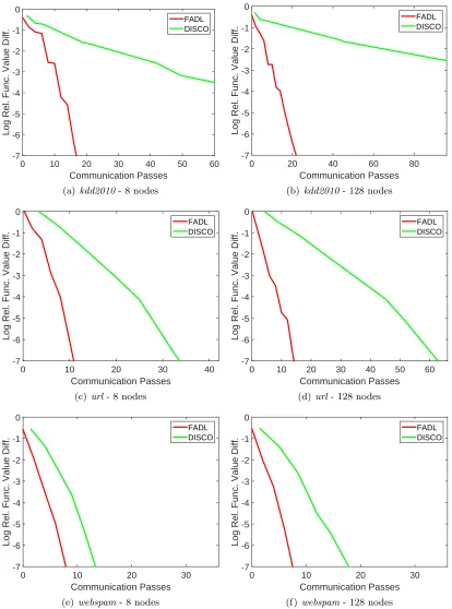
4.8. Comparison of FADL against DiSCO
difference being quite large on datasets such as kdd2010. In terms of total computing time, the superiority of FADL turns out to be even better than what is seen in the plots of communication passes. This is because DiSCO requires more extensive computational steps than FADL within one communication pass.
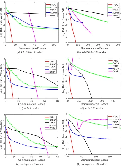
4.9. Comparison of FADL against TERA, ADMM, CoCoA and DANE
Having made the best choice of settings for the methods, we now evaluate FADL against TERA, ADMM, CoCoA and DANE in more detail. We do this using three sets of plots. We give details only for P = 8 andP = 128 to give an idea of how performance varies for small and large number of nodes.
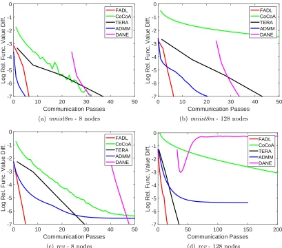
1. Communication passes. We plot the variation of the training objective function as a function of the number of communication passes. For thex-axis we prefer the number of communication passes instead of the number of outer iterations since the latter has a different meaning for different methods while the former is quite uniform for all methods. Figures 6 and 7 give the plots respectively for the large dimensional (m large) datasets (kdd2010, url and webspam) and medium/small dimensional (m medium/small) datasets (mnist8m andrcv).
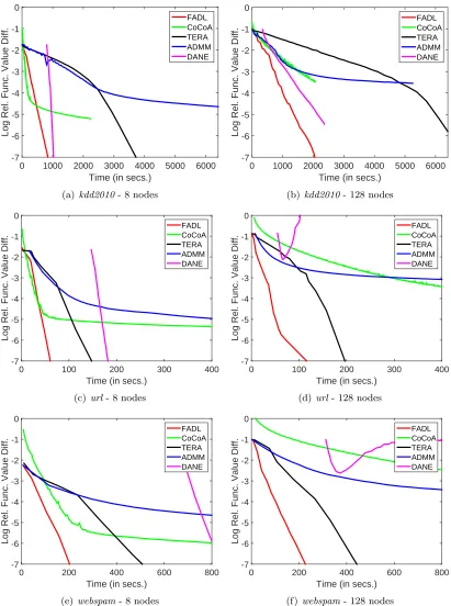
2. Time. We plot the variation of the training objective function as a function of the ac-tual solution time. Figures 8 and 9 give the plots respectively for the large dimensional and medium/small dimensional datasets.
3. Speed-up over TERA.TERA is an established strong baseline method. So it is useful to ask how other methods fare relative to TERA and study this as a function of the number of nodes. For doing this we need to represent each method by one or two real numbers that indicate performance. Since generalization performance is finally the quantity of interest, we stop a method when it reaches within 0.1% of the steady state AUPRC value achieved by full, perfect training of (8) and record the following two measures: the total number of communication passes and the total time taken. For each measure, we plot the ratio of the measure’s value for TERA to the corresponding measure’s value for a method, as a function of the number of nodes, and repeat this for each method. Larger this ratio, better is a method; also, ratio greater than one means a method is faster than TERA. Figures 10 and 11 give the plots for all the five datasets.
Let us now use these plots to compare the methods. In the plots, DANE starts later than other methods due to the extra work needed for tuning the proximal parameterµ.
4.9.1. Rate of Convergence
Communication Passes
0 10 20 30 40 50 60
Log Rel. Func. Value Diff.
-7 -6 -5 -4 -3 -2 -1 0 FADL DISCO
(a)kdd2010- 8 nodes
Communication Passes
0 20 40 60 80
Log Rel. Func. Value Diff.
-7 -6 -5 -4 -3 -2 -1 0 FADL DISCO
(b) kdd2010- 128 nodes
Communication Passes
0 10 20 30 40
Log Rel. Func. Value Diff.
-7 -6 -5 -4 -3 -2 -1 0 FADL DISCO
(c) url- 8 nodes
Communication Passes
0 10 20 30 40 50 60
Log Rel. Func. Value Diff.
-7 -6 -5 -4 -3 -2 -1 0 FADL DISCO
(d) url- 128 nodes
Communication Passes
0 10 20 30
Log Rel. Func. Value Diff.
-7 -6 -5 -4 -3 -2 -1 0 FADL DISCO
(e)webspam- 8 nodes
Communication Passes
0 10 20 30
Log Rel. Func. Value Diff.
-7 -6 -5 -4 -3 -2 -1 0 FADL DISCO
(f)webspam- 128 nodes
Communication Passes
0 20 40 60 80 100
Log Rel. Func. Value Diff.
-7 -6 -5 -4 -3 -2 -1 0 FADL CoCoA TERA ADMM DANE
(a)kdd2010- 8 nodes
Communication Passes
0 100 200 300 400 500
Log Rel. Func. Value Diff.
-7 -6 -5 -4 -3 -2 -1 0 FADL CoCoA TERA ADMM DANE
(b) kdd2010- 128 nodes
Communication Passes
0 20 40 60 80
Log Rel. Func. Value Diff.
-7 -6 -5 -4 -3 -2 -1 0 FADL CoCoA TERA ADMM DANE
(c) url- 8 nodes
Communication Passes
0 100 200 300 400
Log Rel. Func. Value Diff.
-7 -6 -5 -4 -3 -2 -1 0 FADL CoCoA TERA ADMM DANE
(d) url- 128 nodes
Communication Passes
0 10 20 30 40 50 60
Log Rel. Func. Value Diff.
-7 -6 -5 -4 -3 -2 -1 0 FADL CoCoA TERA ADMM DANE
(e)webspam- 8 nodes
Communication Passes
0 50 100 150
Log Rel. Func. Value Diff.
-7 -6 -5 -4 -3 -2 -1 0 FADL CoCoA TERA ADMM DANE
(f)webspam- 128 nodes
Communication Passes
0 10 20 30 40 50
Log Rel. Func. Value Diff.
-7 -6 -5 -4 -3 -2 -1 0 FADL CoCoA TERA ADMM DANE
(a)mnist8m- 8 nodes
Communication Passes
0 10 20 30 40 50
Log Rel. Func. Value Diff.
-7 -6 -5 -4 -3 -2 -1 0 FADL CoCoA TERA ADMM DANE
(b)mnist8m- 128 nodes
Communication Passes
0 10 20 30 40 50
Log Rel. Func. Value Diff.
-7 -6 -5 -4 -3 -2 -1 0 FADL CoCoA TERA ADMM DANE
(c)rcv- 8 nodes
Communication Passes
0 50 100 150 200
Log Rel. Func. Value Diff.
-7 -6 -5 -4 -3 -2 -1 0 FADL CoCoA TERA ADMM DANE
(d) rcv- 128 nodes
Figure 7: Plots showing the linear convergence of various methods for the two low/medium dimensional datasets.
TERA uses distributed computation only to compute the gradient and so the plots should be unaffected by P. But in the plots we do see differences between the plots for P = 8 and P = 128. This is because of their different initialization (average of one pass SGD solutions from nodes): the initialization with lower number of nodes is better due its smaller variance; note also the better starting objective function value at the start (left most point) forP = 8.
For FADL, the rate is steeper for P = 8 than for P = 128. This steeper behavior for lower number of nodes is expected because the functional approximation in each node becomes better as the number of nodes decreases.
Even though the end convergence rate of ADMM is slow, it generally shows good rates of convergence in the initial stages of training. This is a useful behavior because generalization measures such as AUPRC tend to achieve steady state values quickly in the early stages. This usefulness is seen in Figure 10 too.
DANE has good rates of convergence when P is small (P = 8), but the cost associated with tuning µ makes it poor; note that, if µ is not tuned, that will affect the rate of convergence. DANE tends to be unstable for large P values.
Overall, FADL gives much better rates of convergence (both, in the early training stage as well as in the end stage) compared to TERA, CoCoA, ADMM and DANE methods.14 FADL shows a large reduction in the number of communication passes over TERA, es-pecially when the number of nodes is small. Against CoCoA the trend is the other way: FADL needs a much smaller number of communication passes than CoCoA especially when the number of nodes is large. These observations can also be seen from Figure 10. Clearly CoCoA seems to be very slow with increasing number of nodes.
4.9.2. Time Taken
In the previous analysis we ignored computation costs within each iteration. But these costs play a key role when we analyze overall efficiency in terms of the actual time taken. We study this next. Figures 8 and 9 are relevant for this study. FADL, ADMM, CoCoA and DANE involve much more extensive computations in the inner iterations than TERA; this is especially true when the number of nodes is small because of the large amount of local data in each node. TERA fares much better in the time analysis than what we saw while studying using communication passes only. Thus the gap between TERA and other methods becomes a lot smaller in the time analysis. Compare, for example, TERA and ADMM with respect to communication passes and time. Although ADMM is much more efficient than TERA with respect to the number of communication passes, TERA catches up nicely with ADMM on the time taken.
CoCoA does well sometimes; for example, on kdd2010 and url, when the number of nodes is small, sayP = 8. But it is slow otherwise, especially when the number of nodes is large.
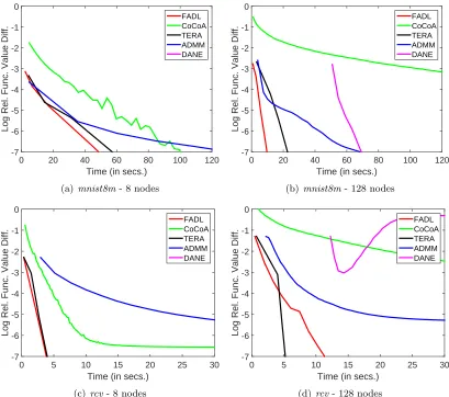
FADL is uniformly better than ADMM with respect to the total time taken. Overall, FADL shows the best performance, performing equally or much better than other methods in different situations. With medium/low dimensional datasets (see Figure 9), communication time is less of an issue and so the expectation is that FADL is less of value for them. Even on these datasets, FADL does equally or better than TERA. DANE is not competitive due to the time involved for tuningµ.
Time (in secs.)
0 1000 2000 3000 4000 5000 6000
Log Rel. Func. Value Diff.
-7 -6 -5 -4 -3 -2 -1 0 FADL CoCoA TERA ADMM DANE
(a)kdd2010- 8 nodes
Time (in secs.)
0 1000 2000 3000 4000 5000 6000
Log Rel. Func. Value Diff.
-7 -6 -5 -4 -3 -2 -1 0 FADL CoCoA TERA ADMM DANE
(b) kdd2010- 128 nodes
Time (in secs.)
0 100 200 300 400
Log Rel. Func. Value Diff.
-7 -6 -5 -4 -3 -2 -1 0 FADL CoCoA TERA ADMM DANE
(c) url- 8 nodes
Time (in secs.)
0 100 200 300 400
Log Rel. Func. Value Diff.
-7 -6 -5 -4 -3 -2 -1 0 FADL CoCoA TERA ADMM DANE
(d) url- 128 nodes
Time (in secs.)
0 200 400 600 800
Log Rel. Func. Value Diff.
-7 -6 -5 -4 -3 -2 -1 0 FADL CoCoA TERA ADMM DANE
(e)webspam- 8 nodes
Time (in secs.)
0 200 400 600 800
Log Rel. Func. Value Diff.
-7 -6 -5 -4 -3 -2 -1 0 FADL CoCoA TERA ADMM DANE
(f)webspam- 128 nodes
Time (in secs.)
0 20 40 60 80 100 120
Log Rel. Func. Value Diff.
-7 -6 -5 -4 -3 -2 -1 0 FADL CoCoA TERA ADMM DANE
(a)mnist8m- 8 nodes
Time (in secs.)
0 20 40 60 80 100 120
Log Rel. Func. Value Diff.
-7 -6 -5 -4 -3 -2 -1 0 FADL CoCoA TERA ADMM DANE
(b)mnist8m- 128 nodes
Time (in secs.)
0 5 10 15 20 25 30
Log Rel. Func. Value Diff.
-7 -6 -5 -4 -3 -2 -1 0 FADL CoCoA TERA ADMM DANE
(c)rcv- 8 nodes
Time (in secs.)
0 5 10 15 20 25 30
Log Rel. Func. Value Diff.
-7 -6 -5 -4 -3 -2 -1 0 FADL CoCoA TERA ADMM DANE
(d) rcv- 128 nodes
Figure 9: Plots showing the time efficiency of various methods for the two low/medium dimensional datasets. Forrcvandmnist8m- 8 nodes, the plot of DANE is invisible since the time taken for tuningµis larger than the time window displayed.
4.9.3. Relative performance of the methods
Figure 11 is relevant for this study. CoCoA shows impressive speed-up over TERA on
Number of Nodes
20 40 60 80 100 120
TERA Comm. Pass / Comm. Pass
0 10 20 30 40 50
60 FADL
CoCoA TERA ADMM DANE
(a) kdd2010
Number of Nodes
20 40 60 80 100 120
TERA Comm. Pass / Comm. Pass
0 5 10 15
FADL CoCoA TERA ADMM DANE
(b) url
Number of Nodes
20 40 60 80 100 120
TERA Comm. Pass / Comm. Pass
0 5 10 15
FADL CoCoA TERA ADMM DANE
(c) webspam
Number of Nodes
20 40 60 80 100 120
TERA Comm. Pass / Comm. Pass
0 2 4 6 8 10 12 14
FADL CoCoA TERA ADMM DANE
(d) mnist8m
Number of Nodes
20 40 60 80 100 120
TERA Comm. Pass / Comm. Pass
0 1 2 3 4 5
6 FADL
CoCoA TERA ADMM DANE
(e) rcv
Number of Nodes
20 40 60 80 100 120
TERA Time / Time
0 5 10 15
FADL CoCoA TERA ADMM DANE
(a) kdd2010
Number of Nodes
20 40 60 80 100 120
TERA Time / Time
0 0.5 1 1.5 2 2.5 3
3.5 FADL
CoCoA TERA ADMM DANE
(b) url
Number of Nodes
20 40 60 80 100 120
TERA Time / Time
0 0.5 1 1.5 2 2.5
3 FADL
CoCoA TERA ADMM DANE
(c) webspam
Number of Nodes
20 40 60 80 100 120
TERA Time / Time
0 1 2 3
4 FADL
CoCoA TERA ADMM DANE
(d) mnist8m
Number of Nodes
20 40 60 80 100 120
TERA Time / Time
0 0.5 1 1.5 2
FADL CoCoA TERA ADMM DANE
(e) rcv
4.9.4. Speed-up as a function of P
Let us revisit Figure 8 and look at the plots corresponding to kdd2010 for FADL.15 It can be observed that the time needed for reaching a certain tolerance, sayLog Rel. Func. Value Diff. = -3, is two times smaller for P = 8 than forP = 128. This means that using a large number of nodes is not useful, which prompts the question: Is a distributed solution really necessary? There are two answers to this question. First, as we already mentioned, when the training data is huge16andthe data is generated and forced to reside in distributed nodes (moving data between machines is not an efficient option), the right question to ask is not whether we get great speed-up, but to ask which method is the fastest. Second, for a given dataset and method, if the time taken to reach a certain approximate stopping tolerance (e.g., based on AUPRC) is plotted as a function of P, it usually has a minimum at a value P >1. Given this, it is appropriate to choose aP optimally to minimize training time. A large fraction of Big data machine learning applications involve periodically repeated model training involving newly added data. For example, in Advertising, logistic regression based click probability models are retrained on a daily basis on incrementally varying datasets. In such scenarios it is worthwhile to spend time to tuneP in an early deployment phase to minimize time, and then use this choice ofP for future runs.
4.9.5. Computation and Communication Costs
Table 2 shows the ratio of computational cost to communication cost for the three high dimensional datasets for all the methods.17 Note that the ratio is small for TERA and so communication cost dominates the time for it. On the other hand, both the costs are well balanced for FADL. Note that ratio varies in the range of 0.625−2.845. This clearly shows that FADL trades-off computation with communication, while significantly reducing the number of communication passes (Figures 6 and 7) and time (Figures 8 and 9).
FADL CoCoA TERA ADMM
kdd2010 1.6333 0.1416 0.1422 1.8499
url 1.3650 0.1040 0.2986 3.4886
webspam 1.2082 0.1570 0.2423 1.2543
Table 2: Ratio of the total computation cost to the total communication cost for various methods which were terminated when AUPRC reached within 0.1% of the AUPRC value for 128 nodes.
15. We choose FADL as an example, but the comments made in the discussion apply to other methods too. 16. The datasets,kdd2010,urlandwebspamare really not huge in theBig datasense. In this paper we used
them only because of lack of availability of much bigger public datasets.
4.10. Experiment on a much larger dataset
To verify the goodness of FADL, we also did an experiment evaluating FADL against other methods, on a large dataset that is more than an order of magnitude bigger than the largest dataset in Table 1. The dataset is the Splice site recognition dataset from the bioinformatics domain (Sonnenburg and Franc, 2010). In this dataset each example is a sequence; we considered all positional features upto 9 grams. This led to a dataset of 49 million features and 50 million examples. The size of the dataset is larger than 0.65 Terabytes. We employed a cluster of 100 nodes to solve this problem. Figure 12 compares the various methods on (a) the reduction of the objective function as a function of communication passes; (b) the reduction of the objective function as a function of time; and (c) the improvement of generalization performance (AUPRC) as a function of time. It is clear that FADL makes great reductions over other methods, on the number of communication passes. FADL is also the best performer when we measure by the time taken. On clusters with slower communication speeds and iteration set-up times, the value of FADL over other methods will be even higher. Interestingly, CoCoA comes out as the next best performer. CoCoA has slower end convergence than FADL, but it shows up equally well in plot (c) on the improvement of generalization performance. As we saw earlier with other datasets, the value of CoCoA varies a lot; for the current scenario of solving the splice site recognition on 100 nodes it seems to be well-suited. FADL, on the other hand, is uniformly good in varying scenarios of several datasets, number of nodes etc.
4.11. Summary
It is useful to summarize the findings of the empirical study.
• FADL gives a great reduction in the number of communication passes, making it clearly superior to other methods in communication heavy settings.
• In spite of higher computational costs per iteration FADL shows the overall best per-formance on the total time taken. This is true even for medium and low dimensional datasets.
• FADL shows a speed-up of 1-10 over TERA, the actual speed-up depending on the dataset and the setting.
• FADL nicely balances computation and communication costs.
5. Discussion
In this section, we discuss briefly, other different distributed settings made possible by our algorithm. The aim is to show the flexibility and generality of our approach while ensuring
glrc.
Communication Passes
0 50 100 150 200 250 300
Log Rel. Func. Value Diff.
-3.5 -3 -2.5 -2 -1.5 -1 -0.5 0
FADL CoCoA ADMM TERA DANE
(a) Communication efficiency (objective function)
Time(in secs.)
0 2000 4000 6000 8000
Log Rel. Func. Value Diff.
-3.5 -3 -2.5 -2 -1.5 -1 -0.5 0
FADL CoCoA ADMM TERA DANE
(b) Time efficiency (objective function)
Time(in secs.)
0 1000 2000 3000 4000 5000
AUPRC
0.46 0.48 0.5 0.52 0.54 0.56
FADL CoCoA ADMM TERA DANE
(c) Time efficiency (AUPRC)
Figure 12: Plots comparing various methods on theSplice site recognition dataset.
Second, the theory proposed in Section 3 holds for feature partitioning also. Suppose, in each nodepwe restrict ourselves to a subset of features,Jp ⊂ {1, . . . , d}, i.e., include the
constraint, wp ∈ {w : w(j) = wr(j) ∀r 6∈ Jp}, where w(j) denotes the weight of the jth
feature. Note that we do not need{Jp}to form a partition. This is useful since important
features can be included in all the nodes.
Gradient sub-consistency. Given wr and Jp we say that ˆfp(w) has gradient
sub-consistency withf atwr on Jp if ∂w∂f(j)(wr) = ∂ ˆ f ∂w(j)(w
r) ∀j∈J p.
Under the above condition, we can modify the algorithm proposed in Section 3 to come up with a feature decomposition algorithm withglrc.
a monotone property, implying that the approximation is convex. The algorithm only has asymptotic linear rate of convergence and it requires the feature partitions to be disjoint. In contrast, our method hasglrcand works even if features overlap in partitions. Moreover, there does not exist any counterpart of our example partitioning based distributed algorithm discussed in Section 3.
Recently Mairal (2013) has developed an algorithm called MISO. The main idea of MISO (which is in the spirit of the EM algorithm) is to build majorization approximations with good properties so that line search can be avoided, which is interesting. MISO is a serial method. Developing a distributed version of MISO is an interesting future direction; but, given that line search is inexpensive communication-wise, it is unclear if such a method would give great benefits.
Our approach can be easily generalized to joint example-feature partitioning as well as non-convex settings.18 The exact details of all the extensions mentioned above and related
experiments are left for future work.
Recently, a powerful divide and conquer approach Hsieh et al. (2014) has been suggested for training kernel methods. The idea is to partition the input space such that the restric-tions of training on the partitioned input spaces are as decoupled as possible. If, in FADL, we had the ability to choose the parts of data that are placed in the nodes, then we would also gain by choosing decoupled partitions. However, in the distributed case, this requires pre-processing as well as shuffling of data, which are expensive.
6. Conclusion
To conclude, we have proposed FADL, a novel functional approximation based distributed algorithm with provable global linear rate of convergence. The algorithm is general and flexible in the sense of allowing different local approximations at the node level, different algorithms for optimizing the local approximation, early stopping and general data usage in the nodes. We also established the superior efficiency of FADL by evaluating it against key existing distributed methods. We believe that FADL has great potential for solving machine learning problems arising in Big data.
Appendix A: Complexity analysis
Let us use the notations of section 3 given around (21). We define the overall cost of any distributed algorithm as
[(c1
nz
P +c2m)T
inner+c
3γm]Touter, (22)
where Touter is the number of outer iterations, Tinner is the number of inner iterations at each node before communication happens and c1 and c2 denote the number of passes over
the data and m-dimensional dot products per inner iteration respectively. For commu-nication, we assume an AllReduce binary tree as described in Agarwal et al. (2011) with
pipelining. As a result, we do not have a multiplicative factor of log2P in our cost19. γ
is the relative computation to communication speed in the given distributed system; more precisely, it is the ratio of the times associated with communicating a floating point number and performing one floating point operation; γ is usually much larger than 1. c3 is the
number ofm-dimensional vectors (gradients, Hessian-vector computations etc.) we need to communicate.
Method c1 c2 c3 Tinner
SQM 2 ≈5−10 1 1
FADL 2 ≈5−7 2 kˆ
Table 3: Value of cost parameters
The values of different parameters for SQM and FADL are given in Table 3. TSQMouter is the number of overall conjugate gradient iterations plus gradient computations. ˆk is the average number of conjugate gradient iterations (for the inner minimization of ˆfp using
TRON) required per outer iteration in FADL. Typically ˆkis between 5 and 20.
Since dense dot products are extremely fast c2m is small compared toc1nz/P for both
the approaches, we ignore it from (22) for simplicity. Now for FADL to have lesser cost than TERA, we can use (22) to get the condition,
2.0(ˆkTFADLouter −TSQMouter)nz P ≤(T
outer
SQM −2TFADLouter)γm (23)
Let us ignore TSQMouter on the left side of this inequality (in favor of SQM) and rearrange to get the looser condition,
nz
m ≤
γP ˆ k
1 2.0(
TSQMouter Touter FADL
−2) (24)
AssumingTSQMouter>3.0TFADLouter, we arrive at the final condition in (21).
Appendix B: Proofs
Proofs of the results in section 2
Let us now consider the establishment of the convergence theory given in section 2.
Proof of Lemma 1. Let ρ(t) = f(wr +tdr) and γ(t) = ρ(t) −ρ(0)−αtρ0(0). Note the following connections with quantities involved in Lemma 1: ρ(t) = fr+1, ρ(0) = fr, ρ0(t) =gr+1·dr andγ(t) =fr+1−fr−αgr·(wr+1−wr). (4) corresponds to the condition γ(t)≤0 and (5) corresponds to the conditionρ0(t)≥βρ0(0).
γ0(t) =ρ0(t)−αρ0(0). ρ0(0)<0. ρ0 is strictly monotone increasing because, by assump-tion A2,
ρ0(t)−ρ0(˜t)≥σ(t−˜t)kdrk2 ∀t,˜t (25)
This implies that γ0 is also strictly monotone increasing and, all four, ρ,ρ0,γ0 and γ tend to infinity ast tends to infinity.
19. Actually, there is another communication term,γb log2P, wherebis the size of first block of
Let tβ be the point at whichρ0(t) =βρ0(0). Sinceρ0(0)<0 andρ0 is strictly monotone
increasing,tβ is unique andtβ >0. This validates the definition in (6). Monotonicity of ρ0
implies that (5) is satisfied ifft≥tβ.
Note that γ(0) = 0 and γ0(0)<0. Also, sinceγ0 is monotone increasing and γ(t) → ∞
ast→ ∞, there exists a uniquetα >0 such that γ(tα) = 0, which validates the definition
in (7). It is easily checked that γ(t)≤0 iff t∈[0, tα].
The properties also implyγ0(tα)>0, which meansρ0(tα)≥αρ0(0). By the monotonicity
of ρ0 we gettα> tβ, proving the lemma.
Proof of Theorem 2. Using (5) and A1,
(β−1)gr·dr≤(gr+1−gr)·dr ≤Ltkdrk2 (26) This gives a lower bound ont:
t≥ (1−β)
Lkdrk2(−g
r·dr) (27)
Using (4), (27) and (1) we get
fr+1 ≤fr+αtgr·dr≤fr− α(1−β)
Lkdrk2 (−g
r·dr)2≤fr−α(1−β)
L cos
2θkgrk2 (28)
Subtractingf? gives
(fr+1−f?)≤(fr−f?)−α(1−β)
L cos
2θkgrk2 (29)
A2 together with g(w?) = 0 implies kgrk2 ≥ σ2kwr −w?k2. Also A1 implies fr−f? ≤ L
2kw
r−w?k2 Smola and Vishwanathan (2008). Using these in (29) gives
(fr+1−f?) ≤ (fr−f?)−2α(1−β)σ
2
L2 cos
2θ(fr−f?)
≤ (1−2α(1−β)σ
2
L2 cos
2θ)(fr−f?) (30)
Letδ = (1−2α(1−β)Lσ22cos2θ). Clearly 0< δ <1. Theorem 2 follows.
Proofs of the results in section 3
Let us now consider the establishment of the convergence theory given in section 3. We begin by establishing that the exact minimizer of ˆfp makes a sufficient angle of descent at wr.
Lemma 5. Let ˆw?p be the minimizer of ˆfp. Letdp = ( ˆw?p−wr). Then
−gr·dp ≥(σ/L)kgrkkdpk (31)
Proof. First note, using gradient consistency and ∇fp( ˆw?p) = 0 that