Averaged Collapsed Variational Bayes Inference
Katsuhiko Ishiguro [email protected]
NTT Communication Science Laboratories NTT Corporation
Kyoto 619-0237, Japan
Issei Sato [email protected]
Graduate School of Frontier Sciences The University of Tokyo
Tokyo 113-0033, Japan
Naonori Ueda [email protected]
NTT Communication Science Laboratories NTT Corporation
Kyoto 619-0237, Japan
Editor:David Blei
Abstract
This paper presents the Averaged CVB (ACVB) inference and offers convergence-guaranteed and practically useful fast Collapsed Variational Bayes (CVB) inferences. CVB inferences yield more precise inferences of Bayesian probabilistic models than Variational Bayes (VB) inferences. How-ever, their convergence aspect is fairly unknown and has not been scrutinized. To make CVB more useful, we study their convergence behaviors in a empirical and practical approach. We develop a convergence-guaranteed algorithm for any CVB-based inference called ACVB, which enables automatic convergence detection and frees non-expert practitioners from the difficult and costly manual monitoring of inference processes. In experiments, ACVB inferences are comparable to or better than those of existing inference methods and deterministic, fast, and provide easier con-vergence detection. These features are especially convenient for practitioners who want precise Bayesian inference with assured convergence.
Keywords: nonparametric Bayes, collapsed variational Bayes inference, averaged CVB
1. Introduction
Bayesian probabilistic models are powerful because they are capable of expressing complex struc-tures underlying data using various latent variables by formulating the inherent uncertainty of the data generation and collection process as stochastic perturbations. To fully utilize such Bayesian probabilistic models, we rely on Bayesian inferences that compute the posterior distributions of the model given the data. Bayesian inferences infer the shapes of the posterior distribution, in contrast to the point estimate inferences such as Maximum Likelihood (ML) inferences and Maximum a Pos-terior (MAP) inference that approximate a complicated parameter distribution by a single parameter (set).
Two Bayesian inference algorithms are frequently used for Bayesian probabilistic models: the Gibbs sampler and variational Bayes (cf. Bishop, 2006; Murphy, 2012). The former guarantees asymptotic convergence to the true posteriors of random variables given infinitely many stochastic
c
samples. Variational Bayes (VB) solutions (cf. Attias, 2000; Blei et al., 2016) often enjoy faster convergence with deterministic iterative computations and massively parallel computation thanks to the factorization. The VB approaches also allow easy and automatic detection of convergence. However, VB yields only local optimal solutions due to its use of approximated posteriors.
We can improve these inference methods by developing collapsed estimators, which integrate some parameters out from inferences. Collapsed Gibbs samplers are one of the best inference solu-tions since they achieve faster convergence and better estimation than the original Gibbs samplers. Recently, collapsed variational Bayes (CVB) solutions have been intensively studied, especially for topic models such as latent Dirichlet allocation (LDA) (Teh et al., 2007; Asuncion et al., 2009; Sato and Nakagawa, 2012) and HDP-LDA (Sato et al., 2012). The seminal paper by Teh and others examined a 2nd-order Taylor approximation of variational expectation (Teh et al., 2007). A simpler 0th-order approximated CVB (CVB0) solution has also been developed as an optimal solution in
the sense of minimizedα-divergence (Sato and Nakagawa, 2012). These papers report that CVB
and CVB0 yield better inference results than VB solutions and even slightly better than exact col-lapsed Gibbs in data modeling (Kurihara et al., 2007; Teh et al., 2007; Asuncion et al., 2009), link prediction, and neighborhood search (Sato et al., 2012).
In this paper, we are interested in the convergence issue of CVB inferences. The convergence
behavior of CVB inferences remains difficult to analyze theoretically, but basically there is no
guar-antee of convergence for general CVB inferences. Interestingly, this problem has not discussed in the literature with one exception (Foulds et al., 2013), where the authors studied the convergence of CVB on LDA. Unfortunately, their proposal is an online stochastic approximation of MAP which is only valid for LDA. The convergence issue of CVB inference is, however, a more general and problematic issue for practitioners who are unfamiliar with, but still want to tackle state-of-the-art machine learning techniques to various models, not limited to LDA. Since there is no theoretically sound way of determining and detecting convergence of CVB inferences, users must manually de-termine the convergence of the CVB inferences: a daunting task for non-experts. In that sense, CVB is less attractive than naive VB and EM algorithms, whose convergences are guaranteed and easy to detect automatically. These reasons motivate us to study the convergence behaviors of CVB
inferences. Even though the problem remains difficult in theory, we take an empirical and a
practi-cal approach to it. We first monitor the naive variational lower bound and the pseudo leave-one-out (LOO) training log likelihood, and then empirically show that the latter may serve as convergence
metrics. Next, we develop a simple and effective technique that assures CVB convergence for
general Bayesian probabilistic models. Our proposed annealing technique, calledAveraged CVB
(ACVB), guarantees CVB convergence and allows automatic convergence detection. ACVB has
two advantages. First, ACVB posterior updates offer assured convergence due to a simple
anneal-ing mechanism. Second, fixed points of the CVB algorithm are equivalent to the converged solution of ACVB, if the original CVB algorithm has fixed points. Our formulation is applicable to any model and is equally valid for CVB as well as CVB0. A convergence-guaranteed ACVB will be the preferred choice for practitioners who want to apply state-of-the-art inference to their problems. In Table 1, we summarize the existing CVB works and this paper, based on applied models and the convergence issue.
Paper Applied model Convergence Comments
Teh et al. (2007) LDA - The seminal paper
Asuncion et al.
(2009)
LDA - Introduces CVB0
Sato and Nakagawa (2012)
LDA - Optimality analysis byα-divergence
Foulds et al. (2013) LDA partially Stochastic approx. MAP rather than
CVB0, only valid for LDA
Kurihara et al.
(2007)
DPM - First attempt at DPM
Teh et al. (2008) HDP - First attempt at HDP
Sato et al. (2012) HDP - Approx. solution
Bleier (2013) HDP - Stochastic approx.
Wan (2013) HMM - First attempt at HMM
Wang and Blunsom (2013)
PCFG - First attempt at PCFG
Konishi et al. (2014) IRM - First attempt at IRM
This paper LDA, IRM X Convergence assurance for any
mod-els
Table 1: CVB-related studies summary: in terms of applied models and convergence
is an infinite mixture model for a relational (network) data where an observation link is governed by two latent variables.
In experiments using several real-world relational datasets, we observe that the Averaged CVB0
(ACVB0) inferences offer good data modeling performances, outperform naive VB inferences in
many cases, and often show significantly better performances than the 2nd-order CVB and its av-eraged version. We also observe that ACVB0 typically converges quickly in terms of CPU time, compared to the 2nd-order CVBs and ACVBs. The ACVB0 achieves competitive results with the 0-th order CVB0 inference, which is known to be one of the best Bayesian inference methods. In addition, the ACVB0 guarantees the convergence of the algorithm while the CVB0 does not. Based on these findings, we conclude that ACVB0 inference is convenient and appealing for practitioners because it shows good modeling performance, assures automatic convergence and has relatively fast computation.
The contributions of this paper are summarized as follows:
1. We empirically study the convergence behaviors of CVB inferences and propose a simple but
effective annealing technique called Averaged Collapsed Variational Bayes (ACVB) inference
that assures the convergence of CVB inferences for all models.
2. We confirm that CVB0 with the above averaging technique (ACVB0) inference offers
The rest of this paper is organized as follows. In the 2nd section, we first introduce Bayesian probabilistic models used in experimental validation. Then we briefly review the variational Bayes and the collapsed variational Bayes inferences. Then we present the convergence issue of the CVB inferences using two sections. In section 3, we first empirically show that we can monitor the con-vergence of the CVB inference by a handy measurement: the pseudo leave-one-out log-likelihood.
In section 4, we propose a simple but effective variant of the CVB, the averaged collapsed variational
Bayes (ACVB) inference that ensure the convergence of the inference process. The 5th section is devoted to experimental evaluations, and the final section concludes the paper.
2. Background
2.1 Generative Models
In experimental validations, we chose two types of different Bayesian probabilistic models. In this
section we first briefly explain them.
2.1.1 LDA
Latent Dirichlet allocation(LDA) (Blei et al., 2003) is a popular Bayesian probabilistic model for topic modeling of Bag-of-Words (BoW) style document data collections. In this paper, we employ LDA as a representative of a model family where an observed word (sample) is governed by a single latent variable.
Assume the observed BoW data collection consists ofDdocuments, where eachd(∈ {1,2, . . . ,D}
)-th document hasNdtokens. A token may choose a value (word) from the set of unique words whose
cardinality isV. Then a probabilistic generative process of LDA is written as follows:
βk |β0∼Dirichlet (β0), (1)
θd |α∼Dirichlet (α), (2)
zd,i|θd∼Discrete (θd), (3)
xd,i |βk,zd,i∼Discrete
βzd,i
. (4)
Topic models including LDA are characterized by the notion of topics. A topic is represented
as a V-dimensional vector whose v-th attribute indicates the mixing ratio of a v-th word, βk, in
Equation (1). We assume the number of topics is given as a hyperparameter, and denote the number
of topics by K and thusk ∈ {1,2, . . . ,K}. A document is formulated as a mixture of topics. The
mixing proportion of theKtopics ford∈ {1,2, . . . ,D}th document isθd, in Equation (2).
zd,i in Equation (3) denotes a topic assignment of the dth document’sith observed word.
Be-cause θ is a K-dimensional vector, zd,i = k ∈ {1,2, . . . ,K}. Throughout our paper, we
inter-changeably choose the 1-of-K representation of Z, wherezd,i = k is equivalently represented by
zd,i,k = 1,zd,i,l,k =0. We generate the observedi-th observation (token) of thed-th document from
aV-dimensional Discrete distribution, as in Equation (4). xd,i = vmeans thei-th token is thev-th
2.1.2 IRM
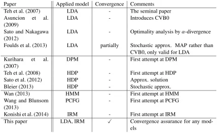
As a slightly complex model family, we also employ the Infinite Relational Model (Kemp et al., 2006), which is an infinite mixture model for a relational (network) data where an observation link is governed by two latent variables: the cluster assignments of the from-node and the to-node.
IRM is an application of the Dirichlet Process Mixture (DPM) (Sethuraman, 1994; Ferguson, 1973; Blackwell and MacQueen, 1973) for relational data. First, assume a binary two-place relation
on the two sets (domains) of objects, namely,D1×D2 → {0,1}, whereD1 ={1, . . . ,i, . . . ,N1}and
D2 ={1, . . . , j, . . . ,N2}. IRM divides the set of objects into multiple clusters based on the observed
relational data matrix of X = {xi,j ∈ {0,1}}. Data entry xi,j ∈ {0,1} denotes the existence of a
relation between a row (the first domain) objecti∈ {1,2, . . . ,N1}and a column (the second domain)
object j∈ {1,2, . . . ,N2}. In an online purchase record case, the first domain corresponds to a user
list, and objectidenotes specific useri. The second domain corresponds to a product item list, and
object jdenotes specific item j. Data entryxi,jrepresents the relation between useriand item j: the
purchase record.
For such data, we define an IRM as follows:
θk,l|ak,l,bk,l ∼Beta ak,l,bk,l, (5)
z1,i|α1 ∼CRP (α1), (6)
z2,j|α2 ∼CRP (α2), (7)
xi,j|Z1,Z2,{θ} ∼Bernoulli
θz1,i,z2,j
. (8)
In Equation (5),θk,l is the strength of the relation between clusterkin the first domain and cluster
lin the second domain. z1,i in Equation (6) and z2,j in Equation (7) denote cluster assignments in
the first and the second domains, respectively. Each domain has its own CRP prior, therefore two
domains may have different numbers of clusters. We generate observed relational dataxi,jfollowing
Equation (8), conditioned by cluster assignments Z1 = {z1,i}
N1
i=1, Z2 = {z2,j}
N2
j=1 and strengthsθ. A
typical example of IRM is shown in Figure 1. The IRM infers the appropriate cluster assignment of
objects Z1 = {z1,i}andZ2 = {z2,j}, given observation relation matrix X = {xi,j}. We can interpret
the clustering as the permutation of object indices to discover the “block” structure (Figure 1 (b)). As a special case, we can build an IRM for a binary two-place relation between the same domain
objectsD×D→ {0,1}. The probabilistic generative model of thesingle-domainIRM is described
as follows:
θk,l|ak,l,bk,l ∼Beta ak,l,bk,l, (9)
zi|α∼CRP (α), (10)
xi,j|Z,{θ} ∼Bernoulli
θzi,zj
. (11)
The generative model clearly shows the difference of amulti-domainIRM (Eqs. (5-8)) anda
single-domainIRM (Eqs. (9-11)). In the latter, there are onlyN objects in domain D, and they serve as
either from-nodes or to-nodes in the network. Object indicesiand jpoint to the same domain. On
the other hand, a multi-domain IRM distinguishes the first domain objectifrom the second domain
object j.
Konishi et al. (2014) first introduced CVB algorithms for the single-domain IRM. However, it
is not applicable when the number of from-nodes and to-nodes are different. Further, its use is
2nd domain object j
2nd domain object j (sorted)
1
st
d
o
ma
in
o
b
je
ct
i
1
st
d
o
ma
in
o
b
je
ct
i
(so
rt
e
d
)
(a) (b)
k = 1
k = 2 k = 3
l = 1 l = 2 l = 3
Figure 1: Example of Infinite Relational Models (IRM): (a) input observationX. (b) a visualization
of inferred clustersZ.
unlike the multi-domain IRM. Even though we focus on the multi-domain IRM, all discussions are also valid for a single-domain IRM.
Lastly, we assume two-place relations throughout this paper, but extension that covers higher-order relations is straightforward.
2.2 Variational Bayes (VB) Inference
It is beneficial to quickly derive a VB solution for comparison with a collapsed VB inference. For the VB inference of LDA and IRM, we maximize the VB lower bound, which is defined as:
L =
Z
q(Z,Φ) logp(X,Z,Φ)
q(Z,φ) dZdΦ, (12)
whereZdenotes all of the hidden variables (assumeZ={Z1,Z2}for the IRM case),Φdenotes all
of the associated parameters (e.g.,αdandβkin LDA,θk,lin IRM),Xdenotes all of the observations,
andq(·)s arevariationalposteriors that approximate the true posteriors. The form of the variational
posteriors are chosen to make the inference algorithm efficient. For example, all variational
posteri-ors are assumed to be independent from each other when the mean-field approximation is employed. The lower bound is derived from the following re-formulation of the marginal log likelihood (model
evidence) p(X) by Jensen’s inequality (Bishop, 2006; Murphy, 2012):
logp(X)=log
Z
p(X,Z,Φ)dZdΦ
=log
Z
q(Z,Φ) p(X,Z,Φ)
q(Z,Φ) dZdΦ
≥
Z
q(Z,Φ) log p(X,Z,Φ)
q(Z,Φ) dZdΦ=L .
Thus maximizing the lower bound by identifying good variational posteriorsqis reasonable in the
is also equivalent to minimizing the Kullback-Leibler divergence between true posteriors p∗ and
variational posteriorsq:
logp(X)=L −
Z
q(Z,Φ) log p(Z,Φ| X)
q(Z,Φ) dZdΦ=L +KL q| p
∗.
We can readily obtain a general update rule of variational posterior q(Z) andq(Φ) (Bishop,
2006; Murphy, 2012). For example, we have the following update rule for the variational posterior
of theith hidden variable:
q(zi)∝exp
Eq(Z\i),q(Φ)logp(X,Z,Φ)
, (13)
whereZ\idenotes all of the hidden variables excluding theith hidden variable. Note that the
varia-tional posterior of a hidden variable is dependent on the current values ofq(Φ), i.e., the variational
posteriors of all of the associated parameters. The resulting update rules boil down to simple
up-dates of the sufficient statistics of the distributions for hidden variables and parameters for LDA and
IRM.
2.3 Collapsed Variational Bayes (CVB) Inference
The general idea of CVB inferences for hierarchical probabilistic models (Kurihara et al., 2007; Teh et al., 2007, 2008; Asuncion et al., 2009; Sato and Nakagawa, 2012; Sato et al., 2012) assumes the
variational posteriors of the hidden variables of the model where theparameters are marginalized
out beforehand. In Equation (12), since parametersΦare not marginalized (collapsed) out, we need to compute their variational posteriors as well. The variational posteriors of the parameters impact the inference results and may increase the risk of being trapped at a bad local optimal point.
CVB inference first marginalizes out the parameters in an exact way (as in a collapsed Gibbs sampler). After that, the remaining hidden variables are assumed to be independent from each other.
This brings two advantages to CVB. First, the effects of the marginalized parameters are correctly
evaluated in CVB while VB approximates them. This means that the variational posteriors com-puted by CVB will approximate the true posteriors better than those of VB. Second, we can reduce the number of unknown quantities to be inferred because the parameters are already marginalized. This makes the inference faster, more stable, and decreases the risk of being trapped in local optimal solutions. Mathematically, it has been proven that the lower bound of CVB is always tighter than that of the original VB (Teh et al., 2007). This means CVB is always a better approximation of the true posterior than VB.
The following is the formal definition of the CVB lower bound:
L [Z]=
Z
q(Z) logp(X,Z)
q(Z) dZ. (14)
This is the same formulation as Equation (12) except for the absense of marginalized parameters. Therefore, a general solution is derived in the same manner as in the VB case:
q(zi)∝exp
Eq(Z\i)logp(X,Z)
. (15)
One difference is that CVB computes the soft cluster assignments ofZ while the collapsed Gibbs sampler computes hard assignments for each process. We repeat this process on all objects. This one sweep of updates corresponds to one iteration of CVB inference.
One problem is that it is difficult to conduct precise update computations for CVB unlike the
original VB, even for such relatively simple Bayesian probabilistic models as LDA and IRM. More
specifically, taking expectations overq(Z\i) require intractable discrete combinatorial computations.
To remedy this issue, CVB inference approximates these expectations by Taylor expansion. If we
denote the expectation of predicatexasa=E[x], we have:
f(x)≈ f(a)+ f0(a) (x−a)+ 1
2f
00
(a) (x−a)2 . (16)
Taking the expectations of both sides of Equation (16) yields the following equation:
E[f(x)]≈E[f(a)]+E[f0(a) (x−a)]+ 1
2E[f
00
(a) (x−a)2]
= f(a)+ 1 2E[f
00
(a) (x−a)2]
= f(E[x])+ 1
2f
00
(E[x])V[x]. (17)
The 0th-order term is constant. The 1st-order term is canceled becausex−abecomes zero by taking
the expectation.Vdenotes the posterior variance.
There are two types of approximations in CVB studies. The originalCVB(Teh et al., 2007)
employs 2nd-order Taylor approximation and considers the variance, as in Equation (17). (Asuncion et al., 2009) revealed that the 0th-order Taylor approximation performs quite well in practice for
LDA. This is called theCVB0solution, which approximates the posterior expectation by
E[f(x)]≈ f(E[x]). (18)
Obviously, the CVB0 solution is simpler than that of the 2nd-order approximation. However it is often superior to the 2nd-order CVB in terms of the perplexity of the learned model (Asuncion et al., 2009; Sato and Nakagawa, 2012; Sato et al., 2012). This may seem counter-intuitive since a 0th-order approximation does not approximate anything. To answer this question, we note that a 0th-order approximation CVB0 is in fact a 1st-order approximation: “CVB1”. Recall that in Equation (17) the 1st-order term vanished. This indicates that the 0th-order expansion is equal to the 1st-order expansion. Moreover, it is reasonable that the 1st-order approximation works well in general cases and indeed may outperform higher-order approximations due to uncertainties within the data and imperfections in inference algorithms.
3. Convergence Issue of CVB
3.1 Our Interest: No Assurance for CVB Convergence
Unfortunately, no theoretical guarantee of CVB convergence has been provided so far, probably
because we cannot correctly evaluate the posterior expectations over Z. What we try to find in
CVB solutions is a stationary point of aTaylor-approximated CVB lower bound; we are not sure
that the procedure actually monotonically improves thetruelower bound. Moreover, it is unknown
whether if the CVB update algorithm has a (algorithmic) fixed point. We are not sure whether the algorithm will even stop after infinitely many iterations. Convergence analysis of CVB inference remains an important open problem in the machine learning field. However, the problem has not been well discussed in the literature though many researchers reported that CVB inference yields better posterior estimations in various cases.
Instead of tackling this problem directly, we study two aspects of CVB convergence in this paper. First we empirically study the convergence behaviors of CVB by monitoring a couple of quantities: a naive VB lower bound and the pseudo leave-one-out log likelihood. We show that the latter is potentially useful for CVB convergence detection. We also propose yet another way to deal with CVB convergence, based on a simple annealing technique. We explain the first aspect in this section and the annealing technique in the next section.
3.2 Assessing Candidate Quantities for CVB Convergence Detection
We cannot correctly compute the true CVB lower bound in Equation (14). Therefore, our first approach is to find some quantities that can serve as proxies of it.
For that purpose, we examine two quantities. The first candidate is an approximation of the naive VB lower bound in Equation (12). The VB lower bound is always a lower bound of the true
CVB lower bound. Given the variational posterior of hidden variablesq(Z), we use this posterior
as a proxy ofq(Z) of the naive VB inference. Computing the variational posteriors of marginalized
parameters yields an evaluation of the naive VB lower bound (Equation 12). Of course, this is not equal to the “true” VB lower bound computed by the naive VB inference, but it may be useful for detecting convergence in CVB inferences.
The second one is the pseudo Leave-one-out (LOO) log likelihood of the training data set. The
CVB solutions (and the Gibbs sampler) compute the predictive distribution of an object, say, z1,i,
in a LOO manner. Therefore, we might be able to detect the convergence of CVB inference by watching these predictive distributions. To simplify the explanation, consider a simple model where
sample xi is associated with hidden variablezi through some probabilistic distributions. A pseudo
LOO log likelihood is an approximation of the entire log likelihood (Besag, 1975):
logp(X| Z)u
X
i
logpxi|X\i,Z
. (19)
We can decompose the above log likelihood as the following simpler sum over samplesi:
X
i
logX
k
pxi,zi=k| X\i,Z\i
. (20)
We can easily confirm thatP
kp
xi,zi =k|X\i,Z\i
is in fact a normalization term of a typical
col-lapsed Gibbs posterior by decomposing joint distributions between xi andzi. One merit of pseudo
version of the collapsed Gibbs solution, requiring the same normalizing term. Thus computing the pseudo LOO log likelihood incurs no extra computation cost for CVB inference.
For example, in the case of IRM, we compute the sum of the r.h.s. of Equation (23) (in the
appendix) over all the possible values of z1,i = k ∈ {1,2, . . . ,K} when we update the variational
posterior ofq(z1,i). Let us denote this sum asC1,i, which corresponds toPkp
xi,zi =k|X\i,Z\i
in
Equation (20). In the same manner, we collectC2,jin the second domain updates as the counterpart
ofC1. The total log sumC = PilogC1,i+PjlogC2,j then serves as a “pseudo” log likelihood of
the training dataset for CVB.
For LDA and IRM, we synthesize small and large artificial data to test the two quantities. We
generated two synthetic Bag-of-Words datasets for LDA. The sizes of these datasets were D =
500,V = 1000,K = 10 (smallersynth 1 data), andD = 1500,V = 5000,K = 40 (larger synth
2 data). Similarly, we generated two synthetic relation datasets for IRM. The sizes and the true
numbers of the clusters of these datasets wereN1= 100,N2 =200,K1 =4,K2 =5 (smallersynth
1data), andN1=1,000,N2=1,500,K1=7,K2=6 (largersynth 2data).
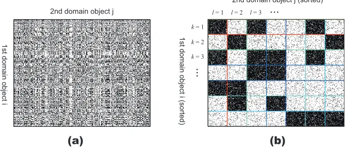
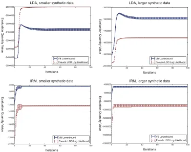
Figures 2 and 3 respectively present the evolutions of these two quantities in CVB and CVB0. The hyperparameters are set in the same procedure of the experimental validations (see the Experi-ment section).
We first notice that the behaviors of the naive VB lower bound (the solid lines) are different in
LDA and IRM. This is not desirable behavior as a cue of convergence detection. In the case of LDA (upper panels in the figures), the VB lower bounds first rise to maximum values, and converge at the lower levels. In the case of IRM (lower panels in the figures), on the other hand, the VB lower bound steadily increases and converges at its highest values. It is not surprising that the naive VB lower bound exhibits such strange behaviors. Recall that CVB inference does not directly increase the VB lower bound, which is a looser bound than that of CVB. We also note that the computation load of the lower bound is much heavier than the CVB updates. Thus there is no strong reason to adopt the naive VB lower bound as a convergence monitoring quantity of CVBs.
In contrast, the pseudo LOO training log likelihood (dashed lines) shows similar behaviors in all cases; monotonically increases its value over the iterations (seemingly) and converges at the maximum values. This behavior is preferable as a cue of the convergence than the case of the lower bound. It is also remarkable that pseudo LOO training log likelihood incurs no extra computation loads over the original CVB updates. Since the property of the quantity more or less resembles the model evidence, the pseudo LOO log likelihood is a good choice for convergence detection.
Based on these results, it is preferable to monitor the pseudo LOO log likelihood to asses the convergence of the CVB inferences. However, we stress that there is no theoretical guarantee that the convergence of the pseudo LOO log likelihood is somehow related to the convergence of the CVB inference.
4. Averaged CVB: Convergence Technique for General CVB
In this section, we propose a more direct and convergence-guaranteed technique for general CVB inferences called Averaged CVB (ACVB) and prove that it reaches the fixed point of the original CVB algorithm, if it exists.
Generally it is fruitful to offer an easy convergence detection algorithm for CVB (not restricted
to LDA and IRM). For many practitioners, manually determine the convergence of the inference
prac-VB Lowerbound Pseudo LOO Log Likelihood
-6000 -8000 -10000 -12000 -14000 -16000 -18000 -20000 -22000 -24000 Eva lu a tio n Q u a n tit y V a lu e Iterations
0 20 40 60 80 100
IRM, smaller synthetic data
VB Lowerbound Pseudo LOO Log Likelihood
-400000 -600000 -800000 -1000000 -1200000 -1400000 -1600000 -1800000 Eva lu a tio n Q u a n tit y V a lu e Iterations
0 20 40 60 80 100
IRM, larger synthetic data VB Lowerbound & Pseudo LOO Log Likelihood (CVB 2nd order)
LDA, smaller synthetic data LDA, larger synthetic data
Iterations
0 20 40 60 80 100
Iterations
0 20 40 60 80 100 -2800000 -2900000 -3000000 -3100000 -3200000 -3300000 -3400000 -3500000 Eva lu a tio n Q u a n tit y V a lu e -1000000 -1200000 -1400000 -1600000 -1800000 -2000000 Eva lu a tio n Q u a n tit y V a lu e VB Lowerbound Pseudo LOO Log Likelihood
VB Lowerbound Pseudo LOO Log Likelihood
Figure 2: Evolution of two quantities over CVB iterations. Solid lines indicate the evolution of naive VB lower bound. Dashed lines indicate the evolution of pseudo LOO log likelihood on training data. Error bars denote the standard deviations. Upper panels: LDA results on two synthetic data. Lower panels: IRM results on two synthetics data.
titioners: they are convergence guaranteed and the convergence is easy to detect. A convergence-guaranteed ACVB motivates users to use CVB inference, which is more precise than naive VB in theory, with automatic computation termination at a guaranteed convergence.
To the best of our knowledge, a paper by Foulds et al. (Foulds et al., 2013) is the only work that proposes convergence-assured CVB inference. This model, which is based on the Robbins and Monro stochastic approximation (Robbins and Monro, 1951), is only valid for LDA-CVB0. More precisely, the solution presented in the paper is a MAP solution, leveraging the fact that the MAP solution closely resembles the CVB0 solution in the case of LDA. They changed the CVB0 update
by ignoring the subtraction of a topic assignment probability vector from sufficient statistics and
manually adjusting the Dirichlet parameters, which makes the CVB0 update is equal to the MAP update in LDA. However, this approach is not valid for IRM because the MAP and CVB0 solutions
are different. On the contrary, the ACVB is valid for any probabilistic models and indeed for both
VB Lowerbound Pseudo LOO Log Likelihood -6000 -8000 -10000 -12000 -14000 -16000 -18000 -20000 -22000 -24000 Eva lu a tio n Q u a n tit y V a lu e Iterations
0 20 40 60 80 100
VB Lowerbound Pseudo LOO Log Likelihood -400000 -600000 -800000 -1000000 -1200000 -1400000 -1600000 -1800000 Eva lu a tio n Q u a n tit y V a lu e Iterations
0 20 40 60 80 100
IRM, smaller synthetic data IRM, larger synthetic data
VB Lowerbound & Pseudo LOO Log Likelihood (CVB 0th order)
LDA, smaller synthetic data LDA, larger synthetic data
Iterations
0 20 40 60 80 100
Iterations
0 20 40 60 80 100
-2700000 -2800000 -2900000 -3000000 -3100000 -3200000 -3300000 -3400000 -3500000 Eva lu a tio n Q u a n tit y V a lu e -1000000 -1100000 -1200000 -1300000 -1400000 -1500000 -1600000 -1700000 -1800000 -1900000 Eva lu a tio n Q u a n tit y V a lu e VB Lowerbound Pseudo LOO Log Likelihood
VB Lowerbound Pseudo LOO Log Likelihood
Figure 3: Evolution of two quantities over CVB0 iterations. Solid lines indicate the evolution of naive VB lower bound. Dashed lines indicate the evolution of pseudo LOO log likelihood on training data. Error bars denote the standard deviations. Upper panels: LDA results on two synthetic data. Lower panels: IRM results on two synthetics data.
4.1 Procedure of ACVB
This technique is based on monitoring the changes ofq(Z). The rationale is simple: it is reasonable
to monitor q(Z) since the CVB solutions are trying to obtain the stationary point of the
Taylor-approximated lower bound with respect toq(Z) , even though we don’t know whether the stationary
point exists, as explained before.
Our solution is a simple annealing technique called Averaged CVB (ACVB) which assures the convergence of CVB solutionDfwe s. We emphasize that the ACVB discussion is not limited to LDA and IRM; this technique is applicable to CVB inference on any model. Also, ACVB is equally valid for CVB (2nd order) and CVB0.
After a certain number of iterations for “burn-in”, we gradually decrease the portion of the variational posterior changes:
¯
q(s+1)= 1− 1 s+1
!
¯
q(s)+ 1 s+1q
(s+1),
or ¯q(S) = 1
S
S
X
s=1
wheresdenotes the iterations after completion of the “burn-in” period, ¯q(s)denotes the “annealed”
variational posterior at the sth iteration,q(s) denotes the variational posterior by CVB inference at
thesth iteration, andS is the total number of iterations. After the “burn-in” period, we monitor the
ratio of changes of ¯qand detect the convergence when the ratio falls below a predefined threshold.
As the final result, we use ¯q(s), notq(s). During the burn-in period, we monitor the changes ofq,
which in most cases quickly converges before entering the annealing process.
Hereafter, we respectively denote the (naive) CVB solution and the CVB0 solution, both for
ACVB, asACVBandACVB0solutions.
4.2 Properties of ACVB
Concerning the convergence of ACVB, there are three points to note. The first is rather evident but makes ACVB useful for practical CVB inference. ACVB assure convergence, and we can easily
detect it by taking the difference of ¯qin successive iterations.
Lemma 1 Averaged variational posterior q¯(s) is convergence-assured: ∀ > 0, ∃S0, s.t.∀S > S0⇒ N1 PN
i=1
q¯
(S)
i −q¯
(S−1)
i
< .
Proof Since
1
S
S
X
s=1
q(s) = 1− 1 S
!
1
S −1 S−1
X
s=1
q(s)+ 1 Sq
(S),
we have 1 S S X s=1
q(s)− 1 S −1
S−1
X
s=1
q(s)
= −1 S 1
S −1 S−1
X
s=1
q(s)+ 1 Sq
(S)
≤ 1 S 1
S −1 S−1
X
s=1
|q(s)|+ 1 S|q
(S)|
≤ 1 S
1
S −1(S −1)+ 1 S = 2 S. Thus, 1 N N X
i=1
1 S S X
s=1
q(is)− 1 S −1
S−1
X
s=1 q(is)
≤ 2 S.
If we setS0= 2, then∀S >S0,
1
N
N
X
i=1
1 S S X
s=1
q(is)− 1 S −1
S−1
X
s=1 q(is)
≤ 2 S < 2
S0 =.
This means
1
N
N
X
i=1
q¯
(S)
i −q¯
(S−1)
i
Thus, we can automatically stop the ACVB inference by a stopping rule based on the difference of the ACVB posteriors.
The second point is also noteworthy and validates the use of ACVB in Bayesian inference.
We can prove that converged ¯q is asymptotically equivalent to the fixed point of the CVB update
algorithm, if it exists (note that it is unclear whether the original CVB update algorithm has a fixed point in theory).
Lemma 2 If variational posterior q(s)converges to a fixed point of the CVB update algorithm, then averaged variational posteriorq¯(s)also converges to the fixed point of the CVB algorithm.
Proof Letq∗be a fixed point of the CVB update algorithm. With this assumption, lim
s→∞q
(s) =q∗
⇔ ∀ >0,∃s0s.t.∀s>s0⇒ |q(s)−q∗|< /2. Here, we define
s0
X
s=1
(q(s)−q∗)
=M>0,
and thus,
lim
s→∞
M
s =0⇔ ∀ >0,∃s 0
0s.t.∀s> s 0 0⇒
M s < /2.
WhenS0=max{s0,s00}, we have
∀S >S0,|q¯(S)−q∗|=
S
X
s=1
1
S(q (s)−q∗
)
< M S +
S
X
s=S0+1
1
S(q (s)−q∗
)
≤/2+
S −S0 S
/2≤/2+/2=.
Therefore,
lim s→∞q¯
(s)=q∗.
Note that the literature fails to resolve whether the CVB algorithm (based on Taylor approximation) has an algorithmic fixed point. However, ACVB remains useful because it assures the convergence of the inference process and will find the true solution if CVB has a fixed point. No solutions to the convergence problem of CVB have ever been published, to the best of our knowledge.
As the third point, we note on the required iteration, S, for the convergence of ACVB. The
Lemma 3 The maximum distance between the averaged variational posteriors of consecutive steps is upperbounded by a term proportional to 1s where s is the number of iterations.
Proof Consider the averaged variational posterior concerning one hidden variable,zi. Also consider
that ¯q(zi) is a real-valued vector on a simplex (say, on aKdimensional simplex). From the definition,
we see:
q¯
(s+1)(z
i)−q¯(s)(zi)
=
1
s+1
q¯
(s)(z
i)−q¯(s+1)(zi)
.
The maximum L2 distance between two simplex vectors is √2. Therefore:
q¯
(s+1)(
zi)−q¯(s)(zi)
=
1
s+1
q¯
(s)(z
i)−q¯(s+1)(zi)
≤
√
2
s+1.
Using this lemma, we roughly expect the number of maximum iterations to satisfy a certain
thresh-old of the averaged CVB posterior differences. For example, we have
q¯
(s+1)(z
i)−q¯(s)(zi)
<
1.4×10⁻³ with s = 1000 iterations, and
q¯
(s+1)(z
i)−q¯(s)(zi)
< 1.0×10
−4 with s = 14000
it-erations. We can use these s as the number of maximum iterations for running the program. In
practice we typically need much fewer iterations to achieve the designed threshold.
5. Experiments
This section presents our experimental validations. In summary, we obtained the following results.
1. For almost all the datasets, CVB and ACVB inferences achieved better modeling performance than the naive VB, in both LDA and IRM.
2. CVB0 and ACVB0 inferences often performed significantly better than their 2nd-order coun-terparts.
3. The computations of the CVB0 and ACVB0 inferences are generally faster than the other VB-based methods.
5.1 Procedure
We compared the performance of the proposed averaged CVB solutions (ACVB, ACVB0) with
naive variational Bayes (VB) and CVB solutions (CVB,CVB0), which are the baseline
determin-istic inferences. As a reference, we also include comparisons with the collapsed Gibbs samplers (Gibbs) with a small number of iterations.
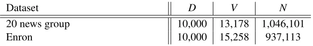
Dataset D V N
20 news group 10,000 13,178 1,046,101
Enron 10,000 15,258 937,113
Table 2: Dataset sizes used in our LDA experiments.
of p(zi = k). In the case of Gibbs, we performed hard assignments ofzi = kto the most weighted
cluster. For the VB, CVB, CVB0, ACVB, and ACVB0 solutions, we normalized the assigned
weights. For the LDA experiments, we set the number of topics asK∈ {50,100,200}. For the IRM
experiments, all of the inferences except Gibbs require a number of truncated clusters a priori. To
assess the effect of the truncation level, our experiments examinedK1 = K2 = K ∈ {20,40,60}. In
practice, we just need to prepare a sufficiently largeKto handle data complexity.
We compared the performance of the inference methods by test data perplexity for LDA and by the averaged test data marginal log likelihood for IRM. Given an observation dataset, we excluded roughly 10% of the observations from the inference as held-out test data. After the inference was finished, we computed the perplexity or the marginal log likelihoods of the test data. The test data were randomly sampled for each run. The perplexity and the log likelihood were computed for 20
runs with different initialization and hyperparameter settings.
In the experiments, we set the maximum numbers of inference iterations and iterated the infer-ences until we reached that maximum. Then we reported the final values of the perplexities (for LDA) or the averaged log likelihood (for IRM) as well the evolutions of these values versus the CPU times.
For the reference Gibbs sampler on LDA, we iterated the sampling procedure 1,000 times and
discarded the first 100 iterations as the burn-in period. For the reference Gibbs sampler on IRM, we
iterated the sampling procedure 3,000 times and discarded the first 1,500 iterations as the burn-in
period.
5.2 Datasets
For our experiments, we prepared several real-world datasets that allowed us to assess the inference performance at several scales and densities.
For the LDA experiments we employed two popular real-world datasets and converted them to the BoW format.
The first dataset is the20 news groupcorpus (Asuncion et al., 2009; Sato and Nakagawa, 2012),
including randomly chosenD=10,000 documents with a vocabulary sizeV =13,178. The second
dataset is theEnronemail corpus (McCallum et al., 2005) including randomly chosenD=10,000
documents with a vocabulary size ofV = 15,258. Stop words were eliminated. Note the reference
materials for detailed information of these datasets. The data sizes and densities are summarized in Table 5.2.
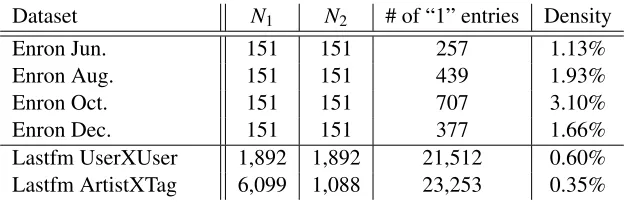
For the IRM experiments, we collected small and large real-world datasets. We explain them more closely since the IRM and the relational data analysis are probably less common than the LDA and the topic model researches for many readers.
Dataset N1 N2 # of “1” entries Density
Enron Jun. 151 151 257 1.13%
Enron Aug. 151 151 439 1.93%
Enron Oct. 151 151 707 3.10%
Enron Dec. 151 151 377 1.66%
Lastfm UserXUser 1,892 1,892 21,512 0.60%
Lastfm ArtistXTag 6,099 1,088 23,253 0.35%
Table 3: Dataset sizes used in our IRM experiments.
extracted monthly e-mail transactions for 2001. The dataset containsN =N1= N2 =151 company
members of Enron. xi,j = 1(0) if there is (not) an e-mail sent from memberito member j. Out of
twelve months, we selected the transactions of June (Enron Jun.), August (Enron Aug.), October
(Enron Oct.), and December (Enron Dec.).
The second real-world relational dataset is the Lastfm dataset1, which contains several records
for the Last.fm music service, including lists of most listened-to musicians, tag assignments for
artists, and friend relations among users. We employed the friend relations amongN = N1= N2 =
1892 users (Lastfm UserXUser). xi,j =1(0) if there is (not) a friend relation from userito user j.
This dataset has ten times more objects and 100 times more matrix entries than the Enron dataset.
We also employed the artist-tag relations between 17,632 artists and 11,946 tags. Since the relation
matrix is too large for Gibbs and naive VB inference, we truncated the number of artists and tags. The original observations were the co-occurrence counts of (artist name, tag) pairs. We binarized the observations as to whether the (artist name, tag) pair counts exceeded; we ignore singletons of (artist name, tag). If the counts exceeded 1, then the observation entries were set to 1; otherwise, they were set to 0. Then all the rows (artists) and columns (tags) that have no “1” entries were
removed. The resulting binary matrix consisted ofN1=6,099 artists andN2=1,088 tags (Lastfm
ArtistXTag). xi,j =1(0) if artistiis (not) assigned tag word jmore than once. The data sizes and densities are summarized in Table 5.2.
5.3 Results
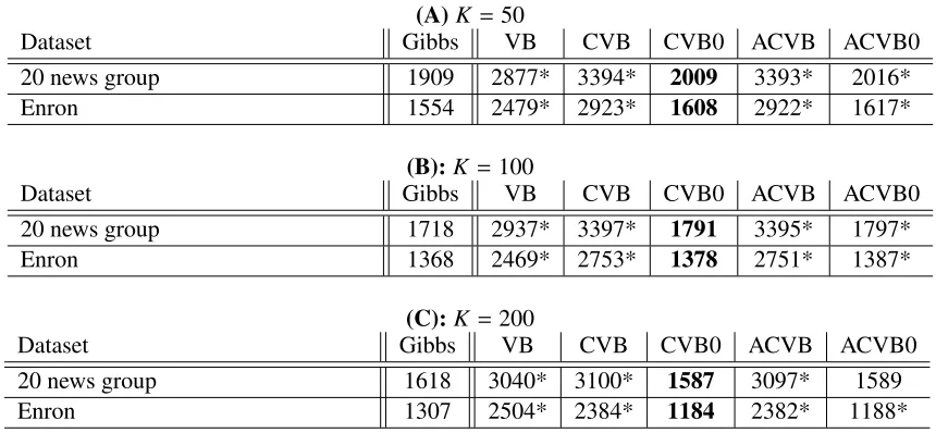
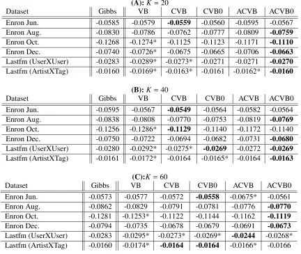
We start by presenting the numerical performances of the inferences. For LDA, we present the per-plexities after 150 iterations in Table 5.3. For IRM, we present the averaged test data log likelihood after 200 iterations in Table 5.3. The results of the best setup are presented for each solution. In
addition, we conducted statistical significance tests usingt-tests.
First, we review the results of the deterministic (VB-based) inference methods on LDA. CVB0
and ACVB0 inferences always outperformed the naive VB, CVB, and ACVB for LDA2. These
results are in good accordance with existing CVB researches. The 2nd-order CVB and ACVB inferences often performed worse than the naive VB. (Asuncion et al., 2009) reported that the
supe-riority of CVB inference over naive VB gradually diminishes as the number of topicsK increases
to roughly more than 100. Our results are probably related to this report.
1. Provided by HetRec2011. http://ir.ii.uam.es/hetrec2011/
(A)K=50
Dataset Gibbs VB CVB CVB0 ACVB ACVB0
20 news group 1909 2877* 3394* 2009 3393* 2016*
Enron 1554 2479* 2923* 1608 2922* 1617*
(B):K=100
Dataset Gibbs VB CVB CVB0 ACVB ACVB0
20 news group 1718 2937* 3397* 1791 3395* 1797*
Enron 1368 2469* 2753* 1378 2751* 1387*
(C):K =200
Dataset Gibbs VB CVB CVB0 ACVB ACVB0
20 news group 1618 3040* 3100* 1587 3097* 1589
Enron 1307 2504* 2384* 1184 2382* 1188*
Table 4: Test perplexity on LDA (10% test data) after 150 iterations. Smaller values are better. Boldface indicates the best method within deterministic methods and is significantly
bet-ter than method(s) marked with ∗(byt-test, p = 0.05). Numbers of Gibbs sampler are
computed after 1,000 iterations. Upper panel: K = 50, middle panel: K = 100, lower
panel:K =200.
CVB0 significantly outperformed ACVB0 in most cases, given the same number of inference iterations. However, ACVB0 provides an easy convergence detection scheme with some theoretical
supports, while CVB0 has no such mechanism3. In that sense there is no strong reason to choose
CVB0 instead of the convergence-guaranteed ACVB0.
Second, we examine the IRM results. For IRM, the CVB and ACVB inferences are significantly better than naive VB in many cases. The ACVB0 inference especially often significantly
outper-formed the other VB-based methods when K is small. One possible reason is that the averaged
posteriors are smoothed versions of the original CVB posteriors. This smoothing may work well for sparse relational data, where inferred solutions tens to be peaky. This result serves as a good reason to adopt ACVB(0) inference: ACVB not only assures the termination of inference algorithm, but also provides better inference solutions than the original CVB in IRM cases.
Third and finally, we compared the performance of the ACVBs and the Collapsed Gibbs
sam-pler. Interestingly, 1,000 iterations of collapsed Gibbs on LDA performed significantly better than
ACVBs, and 3,000 iterations of the collapsed on IRM did not work as well as expected. We believe
this basically depends on the complexity of the model. LDA is a simple probabilistic model. Thus
1,000 iterations of the collapsed Gibbs are adequate for obtaining good posterior computations.
However, IRM is a relatively more complex model than IRM, especially because of the existence
of two hidden variables (z1,z2) for one observation. This indicates that the (A)CVB inference
al-gorithms on IRM are more likely to be trapped at bad local optima, whereas the collapsed Gibbs
sampler yielded stable but not good solutions regardless of the initial Ks. As reported in (Albers
et al., 2013), the collapsed Gibbs for IRM requires millions of iterations to obtain better results.
(A):K =20
Dataset Gibbs VB CVB CVB0 ACVB ACVB0
Enron Jun. -0.0585 -0.0579 -0.0559 -0.0560 -0.0595 -0.0567
Enron Aug. -0.0830 -0.0786 -0.0762 -0.0777 -0.0809 -0.0759
Enron Oct. -0.1268 -0.1274* -0.1125 -0.1123 -0.1171 -0.1110
Enron Dec. -0.0740 -0.0726* -0.0675 -0.0665 -0.0706 -0.0663
Lastfm (UserXUser) -0.0283 -0.0289* -0.0273* -0.0271 -0.0271 -0.0270
Lastfm (ArtistXTag) -0.0160 -0.0169* -0.0163* -0.0161 -0.0162* -0.0160
(B):K=40
Dataset Gibbs VB CVB CVB0 ACVB ACVB0
Enron Jun. -0.0595 -0.0567 -0.0549 -0.0564 -0.0582 -0.0564
Enron Aug. -0.0838 -0.0808 -0.0770 -0.0753 -0.0819 -0.0769
Enron Oct. -0.1256 -0.1286* -0.1129 -0.1140 -0.1172 -0.1140
Enron Dec. -0.0750 -0.0722 -0.0694 -0.0682 -0.0731 -0.0680
Lastfm (UserXUser) -0.0280 -0.0292* -0.0275* -0.0269 -0.0272 -0.0269
Lastfm (ArtistXTag) -0.0161 -0.0172* -0.0164 -0.0165* -0.0164 -0.0163
(C):K =60
Dataset Gibbs VB CVB CVB0 ACVB ACVB0
Enron Jun. -0.0573 -0.0577 -0.0572 -0.0558 -0.0675* -0.0561
Enron Aug. -0.0862 -0.0829 -0.0791 -0.0781 -0.0776 -0.0770
Enron Oct. -0.1281 -0.1253* -0.1122 -0.1144 -0.1162 -0.1119
Enron Dec. -0.0794 -0.0735 -0.0678 -0.0679 -0.0691 -0.0673
Lastfm (UserXUser) -0.0283 -0.0295* -0.0273* -0.0269* -0.0244 -0.0268*
Lastfm (ArtistXTag) -0.0160 -0.0174* -0.0164 -0.0164 -0.0166* -0.0166
Table 5: Marginal test data log likelihood per test data entry (10% test data) on IRM after 200 iter-ations. Larger values are better. Boldface indicates the best method within deterministic
methods and is significantly better than method(s) marked with ∗(byt-test, p = 0.05).
Numbers of the Gibbs sampler are computed after 3,000 iterations. Upper panel:K =20,
middle panel:K=40, lower panel: K =60.
Thus it is perfectly possible that a collapsed Gibbs outperformed all the VB-based techniques, given more sophisticated sampling techniques and many more iterations.
Our results demonstrate one point of contention. The ACVB and CVB inferences are signifi-cantly better than naive VB inference for almost all the IRM cases. This apparently conflicts with a former IRM-CVB study (Konishi et al., 2014) for single-domain IRMs. They reported that CVB inference is inferior to VB for sparse relational data. However, in our experiments, VB never outper-formed ACVB or CVB. Our speculation is that this is due to the model structure of the multi-domain IRM (the focus of this paper) and the single-domain IRM in Konishi et al. (2014). In the observation process of a multi-domain IRM (Equation 8), two hidden variables from two independent domains
other hand, in the case of a single-domain IRM (Equation 11), two hidden variables from the same
(and the sole) domain interact (i.e.ziandzj). Given that LDA has no such variable interactions, we
believe the multi-domain IRM is one step closer to LDA than the single-domain IRM in terms of interaction complication. Therefore, perhaps the behaviors of the (A)CVB and VB inferences in the multi-domain IRM resembles the LDA cases: CVB is superior to VB.
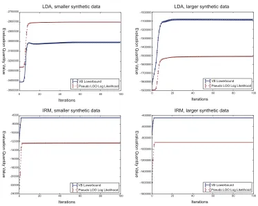
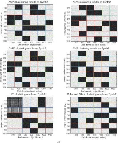
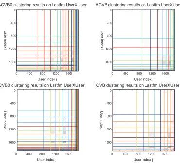
Figures 4 and 5 present examples of the clustering attained for theSynth2andLastfm UserXUser
data inK=60. All of the object indices in the figures are sorted so that the objects are grouped into
blocks. The horizontal and vertical color lines respectively indicate the borders of the object clusters
for first domainkand second domainl. We show the MAP assignments and assign an object to the
cluster with the highest posterior probability.
Finally, we show a few plots of performance measures over CPU time. Figure 6 illustrates the
time evolution of the test data perplexity of LDA on different data sets. Figure 7 illustrates the time
evolution of the test data likelihood of IRM on different data sets. We refrain from presenting the
CPU time evolutions of our naive implementations of the collapsed Gibbs samplers, since there is a
number of very efficient sampling methods for LDA (Li et al., 2014).
We observe that the ACVB0 and CVB0 inferences generally proceed faster than the other in-ference methods. Combined with assured convergence and the good numerical performances, we conclude that the ACVB0 solution is a good inference choice for practical usages.
6. Conclusion
In this paper, we proposed an Averaged Collapsed Variational Bayes (ACVB) inference, which is a convergence-guaranteed and useful deterministic inference algorithm that is expected to replace naive VB in practical applications.
We studied the convergence aspect of CVB inference in two ways to address its open problem. We started by examining two possible convergence metric candidates for CVB solutions. Next,
we proposed a simple and effective annealing technique, Averaged CVB (ACVB), to assure the
convergence of CVB solutions. ACVB posterior updates offer assured convergence due to their
simple annealing mechanism. Moreover, the fixed point of the original CVB update algorithm is equivalent to the converged solution of ACVB, if the CVB algorithm has a fixed point (an issue unresolved in the literature). ACVB is applicable to any model and is equally valid for CVB and CVB0.
In experiments using several real-world relational data sets, we concluded that the Averaged
CVB0 (ACVB0) inference offers the following impressive performances. It outperforms naive VB
inference in many cases and often shows significantly better performances than 2nd-order CVB and its averaged version. ACVB0 typically converges faster than the 2nd-order CVB and ACVB. ACVB0 achieves competitive results with 0-th order CVB0 inference, which is one of the best Bayesian inference methods. In addition, ACVB0 guarantees the convergence of the algorithm while CVB0 does not. Based on these findings we conclude that ACVB0 is an appealing Bayesian inference method for practitioners, who needs precise posterior inferences with guaranteed compu-tational convergences.
ACVB clustering results on Synth2
100
200 400 600 800 1000 1200 1400
200 300 400 500 600 700 800 900 1000
2nd domain object index j
1 st d o ma in o b je ct in d e x i 1400
200 400 600 800 1000 1200
100 200 300 400 500 600 700 800 900 1000
2nd domain object index j
1 st d o ma in o b je ct in d e x i
ACVB0 clustering results on Synth2
200 400 600 800 1000 1200 1400
100 200 300 400 500 600 700 800 900 1000
2nd domain object index j
1 st d o ma in o b je ct in d e x i
VB clustering results on Synth2
200 400 600 800 1000 1200 1400
100 200 300 400 500 600 700 800 900 1000
2nd domain object index j
1 st d o ma in o b je ct in d e x i
Collapsed Gibbs clustering results on Synth2 CVB clustering results on Synth2
100
200 400 600 800 1000 1200 1400
200 300 400 500 600 700 800 900 1000
2nd domain object index j
1 st d o ma in o b je ct in d e x i 1400
200 400 600 800 1000 1200
100 200 300 400 500 600 700 800 900 1000
2nd domain object index j
1 st d o ma in o b je ct in d e x i
CVB0 clustering results on Synth2
1400
200 400 600 800 1000 1200
100 200 300 400 500 600 700 800 900 1000
2nd domain object index j
1 st d o ma in o b je ct in d e x i
Ground truth on Synth2
ACVB0 clustering results on Lastfm UserXUser
User index j 400
1200
1600 800
400 800 1200 1600
0 0
U
se
r
in
d
e
x
i
ACVB clustering results on Lastfm UserXUser
User index j 400
1200
1600 800
400 800 1200 1600
0 0
U
se
r
in
d
e
x
i
VB clustering results on Lastfm UserXUser Collapsed Gibbs clustering results on Lastfm UserXUser
User index j 400
1200
1600 800
400 800 1200 1600
0 0
U
se
r
in
d
e
x
i
User index j 400
1200
1600 800
400 800 1200 1600
0 0
U
se
r
in
d
e
x
i
CVB0 clustering results on Lastfm UserXUser
User index j 400
1200
1600 800
400 800 1200 1600
0 0
U
se
r
in
d
e
x
i
CVB clustering results on Lastfm UserXUser
User index j 400
1200
1600 800
400 800 1200 1600
0 0
U
se
r
in
d
e
x
i
Figure 5: MAP clustering assignments of Lastfm UserXUser data set. All object indices are
Enron, K = 200
better
CPU time [sec]
T
e
st
p
e
rp
le
xi
ty
VB CVB CVB0
ACVB0 ACV0
101 102 103 104 2000
2500 3000 3500 4000 4500
1500 1000
20news, K = 50
better
CPU time [sec]
T
e
st
p
e
rp
le
xi
ty
VB CVB CVB0
ACVB0 ACV0
101 102 103 104 2000
2500 3000 3500 4000 4500 5000
20news, K = 200
better
CPU time [sec]
T
e
st
p
e
rp
le
xi
ty
VB CVB CVB0
ACVB0 ACV0
101 102 103 104 2000
2500 3000 3500 4000 4500 5000
1500
105
Enron, K = 100
better
CPU time [sec]
T
e
st
p
e
rp
le
xi
ty
VB CVB CVB0
ACVB0 ACV0
101 102 103 104 2000
2500 3000 3500 4000 4500
1500 1000
Enron Aug., K = 60 Enron Dec., K = 40
Lasfm UserXUser, K = 20 Lasfm ArtistXTag, K = 60
better A ve ra g e d T e st D a ta lo g li ke lih o o d
10-2 10-1 100 102
-0.095 -0.085 -0.080 -0.075 -0.070 -0.065 -0.100 101 CPU time [sec]
10-2 10-1 100 101 102 CPU time [sec]
-0.105 -0.110 -0.090 better A ve ra g e d T e st D a ta lo g li ke lih o o d -0.20 -0.15 -0.10 -0.05 -0.30 -0.25
100 101 102 103 105 CPU time [sec]
104 better A ve ra g e d T e st D a ta lo g li ke lih o o d -0.034 -0.032 -0.030 -0.028 -0.026 -0.038 -0.036
101 102 103 105 CPU time [sec]
104 better A ve ra g e d T e st D a ta lo g li ke lih o o d -0.045 -0.035 -0.030 -0.025 -0.020 -0.015 -0.050 -0.040 VB CVB CVB0 ACVB0 ACV0 VB CVB CVB0 ACVB0 ACV0 VB CVB CVB0 ACVB0 ACV0 VB CVB CVB0 ACVB0 ACV0
Gibbs samplers for IRM. It is also important to explore efficient CVB algorithms for more
ad-vanced models such as MMSB and its variants (Airoldi et al., 2008; Miller et al., 2009; Griffiths
and Ghahramani, 2011). Aside from the representation of multiple cluster assignments, few studies have addressed other issues. For example, (Fu et al., 2009; Ishiguro et al., 2010) focused on the dynamics of network evolution in the context of stochastic blockmodels (MMSB and IRM). Subset IRM (Ishiguro et al., 2012) is another extension of IRM that automatically filters out nodes from the clustering if they are not very informative for grouping. Applying CVB to these models might make it easier for practitioners to examine the depth of various relational data.
Appendix A. CVB inference algorithm for multi-domain IRM
The IRM model in this paper is a multi-domain model where observation xi,j is governed by row
latent variable z1,i and column latent variable z2,j. Since we distinguish the row and the column
objects, there areN1+N2latent variables.
The CVB inference of IRM was first studied in (Konishi et al., 2014). However, their paper
focused on a single-domain model, where the observation matrix is a N × N square matrix and
the cluster assignment is only defined on N objects without distinguishing rows and columns. Its
CVB scheme is slightly different from the multi-domain IRM, which is our focus in this paper. For
readers’ convenience, we briefly describe the CVB posteriors for multi-domain IRMs. Since we do not fully explain the actual update rules, readers are referred to (Konishi et al., 2014) to obtain them. The CVB inference procedure resembles collapsed Gibbs sampling more than ordinary VB inference. We take one object from the model, recompute the posterior of the object cluster
assign-ment, and put it back in the model. One difference is that CVB computes the soft cluster assignments
ofZ = {Z1,Z2}, while the Gibbs sampler computes hard assignments for each process. We repeat
this process on all the objects, and one iteration(sweep) of CVB inference completes.
Next we derive the update rule of the hidden cluster assignment of the first domainz1,i. First,
we modify the representation of the CVB lower bound. The integral is replaced by the summation
becauseZis discrete:
L h
z1,i,Z\(11 ,i),Z2
i
=X
z1,i X
Z\1(1,i),Z2
q z1,iq
Z\(11 ,i)q(Z2) log
pX(1,i),X\(1,i),z 1,i,Z
\(1,i) 1 Z2
q z1,iq
Z\(11 ,i)q(Z2)
=X
z1,i
EZ\(1,i)
1 ,Z2
q z1,i
n
logpX(1,i)|X\(1,i),z1,i,Z
\(1,i) 1 ,Z2
+logpz1,i|Z
\(1,i) 1
−logq z1,i
+(Terms that are not related to z1,i)
o
. (22)
X(1,i) = {xi,·} denotes the set of all the observations concerning object iof the first domain. The
remaining observations, the hidden variables excluding z1,i, and the statistics computed on these
data, are denoted by\(1,i).Ex[y] indicates the expectations ofyon the variational posterior ofx.
Taking the derivative of Equation (22) w.r.t.q(z1,i) and equating it to zero, we have the following
update rule forq(z1,i):
q z1,i∝exp
EZ\(1,i)
1 ,Z2
h
logpX(1,i)|X\(1,i),z1,i,Z\(11 ,i),Z2
i
+EZ\(1,i) 1 ,Z2
h
logpz1,i|Z\(11 ,i)
i
To evaluate the above equation, we first need to compute the arguments of the expectations. We
employ finite truncation of the Stick breaking process (Sethuraman, 1994) as a prior of Z. With
straightforward computations we have the following (cf. (Konishi et al., 2014)):
pz1,i =k|Z\(11 ,i)
= m
\(1,i) 1,k +1
m1\(1,k,i)+M1\(1,k,i)+α1+1
k−1
Y
k0=1
M\1(1,k0,i)+α1 m\(11,k,0i)+M
\(1,i)
1,k0 +α1+1
. (24)
pX(1,i)|z1,i=k,Z
\(1,i) 1 ,Z2,X
\(1,i)
=
K2
Y
l=1 Γ
ak,l+bk,l+n\(1, i)
k,l +N
\(1,i)
k,l
Γ
ak,l+n
\(1,i)
k,l
Γ
bk,l+N
\(1,i)
k,l
Γ
ak,l+n\(1, i)
k,l +n
+(1,i)
k,l
Γ
bk,l+N\(1, i)
k,l +N
+(1,i)
k,l
Γ
ak,l+bk,l+n
\(1,i)
k,l +N
\(1,i)
k,l +n
+(1,i)
k,l +N
+(1,i)
k,l
. (25)
In the above, we introduced the following sufficient statistics:
m1,k = N1
X
i=1
I(z1,i=k)=
N1
X
i=1
z1,i,k, m\(11,k,i)=m1,k−I(z1,i =k), (26)
M1,k = N1
X
i=1
I(z1,i>k)=
K1
X
k0=k+1
m1,k0, M\(1,i)
1,k = M1,k−I(z1,i>k), (27)
nk,l = N1
X
i=1
N2
X
j=1
z1,i,kz2,j,lxi,j, n\(1k,l,i) =nk,l− N2
X
j=1
z1,i,kz2,j,lxi,j, (28)
Nk,l = N1
X
i=1
N2
X
j=1
z1,i,kz2,j,l(1−xi,j), Nk\(1,l,i) =Nk,l− N2
X
j=1
z1,i,kz2,j,l(1−xi,j) (29)
n+k,(1l ,i)=
N2
X
j=1
z2,j,lxi,j, Nk+,(1l ,i)= N2
X
j=1
z2,j,l(1−xi,j). (30)
The final step is to compute intractable expectations with a help of Taylor-expansion approx-imation. Since this step is completely identical with (Konishi et al., 2014) thus we refrain from presenting details.
Appendix B. Numerical Performance after Convergence
In the experiment section, we examined the performances of several inference solutions fixing the number of inference iterations. Based on the evolutions in Figure 6, we think the LDA inferences have already almost reached the converged status with 150 iterations. However, the results of IRM (Figure 7) indicate that the inference may take some additional time until convergence. Then it is natural to ask that how the performances of the inferences change when we keep the algorithm iterates until convergence (on IRM).
We need to decide which parameter/statistics to be monitored to detect convergence. For the VB
(A)K=20
Data Set Gibbs VB CVB CVB0 ACVB ACVB0
Enron Jun. -0.0585 -0.0578 -0.0559 -0.0560 -0.0550 -0.0561
Enron Aug. -0.0830* -0.0797 -0.0763 -0.0777 -0.0772 -0.0748
Enron Oct. -0.1268* -0.1275* -0.1125 -0.1119 -0.1155 -0.1110
Enron Dec. -0.0740* -0.0727* -0.0675 -0.0665 -0.0680 -0.0656
Lastfm (UserXUser) -0.0283* -0.0289* -0.0273* -0.0271 -0.0271 -0.0269
Lastfm (ArtistXTag) -0.0160* -0.0171* -0.0163* -0.0161* -0.0161* -0.0158
(B)K =40
Data Set Gibbs VB CVB CVB0 ACVB ACVB0
Enron Jun. -0.0595 -0.0564 -0.0549 -0.0564 -0.0552 -0.0534
Enron Aug. -0.0838* -0.0809* -0.0769 -0.0753 -0.0736 -0.0765
Enron Oct. -0.1256* -0.1271* -0.1128 -0.1140 -0.1140 -0.1140
Enron Dec. -0.0750* -0.0722 -0.0693 -0.0682 -0.0691 -0.0680
Lastfm (UserXUser) -0.0280* -0.0292* -0.0273* -0.0269 -0.0272 -0.0269
Lastfm (ArtistXTag) -0.0161 -0.0174* -0.0164* -0.0165* -0.0162 -0.0161
(C)K=60
Data Set Gibbs VB CVB CVB0 ACVB ACVB0
Enron Jun. -0.0573 -0.0576 -0.0572 -0.0558 -0.0570 -0.0540
Enron Aug. -0.0862* -0.0826* -0.0791 -0.0780 -0.0750 -0.0759
Enron Oct. -0.1281* -0.1275* -0.1121 -0.1143 -0.1143 -0.1119
Enron Dec. -0.0794* -0.0736 -0.0676 -0.0679 -0.0678 -0.0673
Lastfm (UserXUser) -0.0283* -0.0294* -0.0273* -0.0269* -0.0244 -0.0268*
Lastfm (ArtistXTag) -0.0160 -0.0177* -0.0164* -0.0164* -0.0163* -0.0163*
Table 6: Marginal test data log likelihood per test data entry ( 10% test data) on IRM after conver-gence. Larger values are better. Boldfaces indicate the best method, which is significantly
better than the method(s) marked with∗(byt-test, p = 0.05). The numbers of the Gibbs
sampler is that of after 3,000 iterations. Upper panel: K = 20, middle panel: K = 40,
lower panel:K =60.
in the monitored quantity; if the changes were smaller than 0.001% of the current value of the
quantity, we assumed that the algorithm had converged.
The modeling performances are presented in Table 6. They show the averages of the test data marginal log likelihood after convergence. The results of the best setup are presented for each
solution. In addition, we conducted statistical significance tests usingt-tests.
References
Collapsed variational Bayesian inference for hidden Markov models. InProc. AISTATS, 2013.
Edoardo M. Airoldi, David M. Blei, Stephen E. Fienberg, and Eric P. Xing. Mixed Membership
Stochastic Blockmodels. Journal of Machine Learning Research, 9:1981–2014, 2008.
Kristoffer Jon Albers, Andreas Leon Aagard Moth, Morten Mørup, and Mikkel N. Schmidt. Large
scale inference in the infinite relational model: Gibbs sampling is not enough. InProc. MLSP,
2013.
Arthur Asuncion, Max Welling, Padhraic Smyth, and Yee Whye Teh. On smoothing and inference
for topic models. InProc. UAI, 2009.
Hagai Attias. A variational Bayesian framework for graphical models. InProc. NIPS, 2000.
Jullian Besag. Statistical Analysis of Non-Lattice Data. Journal of the Royal Statistical Society:
Series D, 24(3):179–195, 1975.
Christopher M. Bishop. Pattern Recognition and Machine Learning. Springer-Verlag New York,
2006.
David Blackwell and James B. MacQueen. Ferguson Distributions via Polya urn schemes. The
Annals of Statistics, 1(2):353–355, 1973.
David M. Blei, Andrew Y. Ng, and Michael I. Jordan. Latent Dirichlet Allocation. Journal of
Machine Learning Research, 3:993–1022, 2003.
David M. Blei, Alp Kucukelbir, and Jon D. McAuliffe. Variational Inference: A Review for
Statis-ticians. arXiv, page arXiv:1601.00670v1 [stat.CO], 2016.
Arnim Bleier. Practical collapsed stochastic variational inference for the HDP. In Proc. NIPS
workshop on topic models, 2013.
Thomas S. Ferguson. A Bayesian Analysis of Some Nonparametric Problems. The Annals of
Statistics, 1(2):353–355, 1973.
James Foulds, Levi Boyles, Christopher DuBois, Padhraic Symyth, and Max Welling. Stochastic
collapsed variational Bayesian inference for latent Dirichlet allocation. InProc. KDD, 2013.
Wenjie Fu, Le Song, and Eric P. Xing. Dynamic mixed membership blockmodel for evolving
networks. InProc. ICML, 2009.
Thomas L. Griffiths and Zoubin Ghahramani. The Indian Buffet Process : An Introduction and
Review. Journal of Machine Learning Research, 12:1185–1224, 2011.
Toke Jansen Hansen, Morten Mørup, and Lars Kai Hanse. Non-parametric co-clustering of large
scale sparse nipartite networks on the GPU. InProc. MLSP, 2011.
Katsuhiko Ishiguro, Tomoharu Iwata, Naonori Ueda, and Joshua B. Tenenbaum. Dynamic infinite