Learning Theory of Distributed Regression with Bias
Corrected Regularization Kernel Network
Zheng-Chu Guo [email protected]
School of Mathematical Sciences, Zhejiang University, Hangzhou 310027, P. R. China
Lei Shi [email protected]
Shanghai Key Laboratory for Contemporary Applied Mathematics, School of Mathematical Sciences, Fudan University,
Shanghai 200433, P. R. China
Qiang Wu [email protected]
Department of Mathematical Sciences, Middle Tennessee State University, Murfreesboro, TN 37132, USA
Editor:John Shawe-Taylor
Abstract
Distributed learning is an effective way to analyze big data. In distributed regression, a typical approach is to divide the big data into multiple blocks, apply a base regression algorithm on each of them, and then simply average the output functions learnt from these blocks. Since the average process will decrease the variance, not the bias, bias correction is expected to improve the learning performance if the base regression algorithm is a biased one. Regularization kernel network is an effective and widely used method for nonlinear re-gression analysis. In this paper we will investigate a bias corrected version of regularization kernel network. We derive the error bounds when it is applied to a single data set and when it is applied as a base algorithm in distributed regression. We show that, under certain appropriate conditions, the optimal learning rates can be reached in both situations.
Keywords: Distributed learning, kernel method, regularization, bias correction, error bound
1. Introduction
Data acquisition become much faster and easier as the development of technology. In this big data era, distributed learning has received considerable attention and is shown to be an effective way to analyze data that is so big and cannot be handled by a single machine. Among various distributed learning paradigms, a simple one is to divide the whole data set into multiple blocks, apply a base learning algorithm to each block, and then average the results from different blocks (Rosenblatt and Nadler, 2016; Zhang et al., 2015). This process, though simple, has some advantages. First, it is computationally efficient because the second stage can be easily parallelized. Second, because no mutual communication is required, the data security or confidentiality can be well protected. Last, recent research shows this method is consistent and sometimes reaches optimal learning rate (Zhang et al., 2015; Lin et al., 2017). Thus its asymptotic effectiveness is theoretically guaranteed.
c
In distributed learning the performance highly depends on the selection of the base algorithm in the second stage. Assume a big data set D of N observations is randomly divided into m blocks, D1, D2, . . . , Dm, which are assumed to be of the same size at the
moment so that Di are independent and identically distributed if the entire sample set
D is independently drawn from some unknown distribution ρ. Let ˆf1,fˆ2, . . . ,fˆm be the
estimators obtained by applying a base algorithm on these data blocks. Assume each estimator ˆfihas biasband variancev. Then the mean squared error of ˆfi is mse( ˆfi) =b2+v
while the average estimator
¯
f = 1
m
m
X
i=1
ˆ
fi
has mse( ¯f) =b2+mv.On a single data block the algorithm usually trades off the bias and variance well to achieve the optimal performance. In distributed learning, however, the variance shrinks fast when m is large but the bias keeps unchanging during the average process. In this case, the bias may dominate the learning performance. An algorithm (or a model selection strategy) that is optimal for a single block is not necessarily still optimal for distributed learning. Instead, distributed learning prefers algorithms of small bias as the base learning algorithm on each block. Therefore, when a base learning algorithm is biased, bias correction is expected to play a role to improve the performance. The purpose of this paper is to investigate the application of biased corrected regularization kernel network for distributed regression analysis.
In regression analysis, the data D={(x1, y1),(x2, y2), . . . ,(x|D|, y|D|)}is a set of
obser-vations collected for input variableX of predictors and a scalar response variableY,where
|D|is the sample size of the data setD.Assume they are linked by
yi =f∗(xi) +i, i= 1,2, . . . ,|D|,
where xi comes from a compact metric space (e.g., a bounded subset in Rp), yi ∈R, and i is a zero-mean noise. The target is to recover the unknown true model f∗ as accurate
regression. This will provide a theoretical guarantee for the use of BCRKN from a learning theory perspective.
The rest of this paper will be arranged as follows. In Section 2 we will describe the BCRKN algorithm and state our main results. In particular, we show that BCRKN can achieve the minimax optimal rates in both single data learning and distributed learning. Moreover, BCRKN relaxes the saturation effect of RKN. In Section 3 we discuss the relations of our results with existing work and conduct some comparisons. The proofs of our results are given in Sections 4-8.
2. Main results
Let X denote the input space which is assumed to be a compact metric space. A Mercer kernel onX is a continuous, symmetric, and positive-semidefinite functionK:X × X →R. The function class spanned by {Kx = K(x,·) : x ∈ X } and equipped with the inner
product satisfying hKx, KtiK =K(x, t) forms a pre-Hilbert space. Its completion is called
a reproducing kernel Hilbert space (RKHS)HK associated to the kernelK, with the name
coming after the reproducing property f(x) =hf, K(x,·)iK,∀f ∈ HK. Note that|f(x)| ≤
p
K(x, x)kfkK for all f ∈ HK. Consequently, with κ = supx∈X
p
K(x, x) < ∞, HK can
be embedded intoC(X) andkfk∞≤κkfkK.More other properties of RKHS that will not
be used in this paper can be found in Aronszajn (1950).
Given the data D and the RKHSHK,RKN estimates the true model by
fD,λ= arg min f∈HK
1
|D| |D|
X
i=1
(yi−f(xi))2+λkfk2K, (1)
where λ > 0 is a regularization parameter that trades off the fitting error and model complexity. The well known representer theorem (Wahba, 1990) tells that
fD,λ(x) = |D|
X
i=1
ciK(xi, x)
with the coefficients c = (c1, . . . , c|D|)> satisfying (λ|D|I +K)c = yD where I represents
an identity matrix (or operator), K = (K(xi, xj)) |D|
i,j=1 is the kernel matrix on the input
data xD ={x1, . . . , x|D|} and yD = (y1,· · ·, y|D|)> is the vector of the response data. Let
SD :HK →R|D| be the sampling operator defined by
SDf = (f(x1), . . . , f(x|D|))>, ∀f ∈ HK.
Its dual operator SD∗ is given by
SD∗c=
|D|
X
i=1
ciKxi ∈ HK, ∀c∈R
|D|
.
Then fD,λ has the following operator representation (Smale and Zhou, 2007)
fD,λ= |D|1
λI+|D1 SD∗SD
−1
Note that the operator |D|1 SD∗SD is a sample version of the integral operator
LKf(x) =Et[K(x, t)f(t)] =
Z
X
K(x, t)f(t)dρX(t)
whereρX is the marginal distribution ofρonX.Recall thatLKdefines a compact,
symmet-ric, and positive operator onHK. In the sequel we also use the notationLK,D = |D|1 SD∗SD
and write
fD,λ = (λI+LK,D)−1
1
|D|S ∗ DyD
.
By the aid of operator representation (2), the asymptotic bias of RKN can be charac-terized as −λ(λI+LK)−1f∗.The bias corrected regularization kernel network (BCRKN)
is defined by subtracting a plug-in estimator of the bias (Wu, 2017)
fD,λ] =fD,λ+λ(λI+LK,D)−1fD,λ. (3)
It is also verified in Wu (2017) that
fD,λ] (x) =
n
X
i=1
c]iK(xi, x)
withc]=c+λ λI+n1K−1
c.The effectiveness of BCRKN has been tested empirically by a variety of simulations and real applications in Wu (2017). The main purpose of this paper is to verify its effectiveness in distributed regression from a learning theory perspective.
To perform rigorous error analysis and present our main results, we need some notations and assumptions that are used throughout the paper. Firstly, we assume |y| ≤M almost surely for some constant M > 0. This implies the true regression function f∗ satisfies
kf∗k∞≤M.
Note that we can extend the domain of LK toL2ρX and obtain a compact, symmetric,
and positive operator on L2ρ
X,which will be denoted by L. We can in turn say LK is the restriction ofLonHK.SoLf =LKf forf ∈ HK and we do not need to differentiate them
when operating on functions inHK.Our second assumption is a regularity condition on the
true model:
f∗=Lr(u∗) for some r >0 and u∗ ∈L2ρ
X. (4)
This assumption has been widely used in the literature of learning theory to characterize the approximation ability of HK; see e.g. De Vito et al. (2005); Smale and Zhou (2007); Bauer et al. (2007); Zhang et al. (2015) and many references therein. Recall that L12 is an
isomorphism fromHK onto HK, i.e.
kfkL2
ρX =kL
1
2fkK, forf ∈ HK, (5)
whereHK is the closure ofHK in L2ρ
X.So ifr ≥
1
2, the condition (4) implies f
∗∈ H K.
We shall use the effective dimension N(λ) = Tr((LK+λI)−1LK), that is, the trace of
(LK+λI)−1LK,to measure the complexity ofHKwith respect toρX.We assume that there exist a constantC0 >0 and some 0< β≤1 such that for all λ >0
Again this is a natural and widely used assumption in the literature; see e.g. De Vito et al. (2005); Caponnetto and De Vito (2007); Zhang et al. (2013); Lin et al. (2017).
Assume κ≥1 without loss of generality for otherwise all our statements and proofs are still valid by definingκ= max{1,sup
x∈X
p
K(x, x)}.Denote
B|D|,λ = p2κ
|D|
(
κ
p
|D|λ+
p
N(λ)
)
.
The consistency of RKN as well as BCRKN generally requires the regularization pa-rameter λto be chosen according to the sample size and satisfy λ→ 0 andλ|D| → ∞ as
|D| → ∞.This implies λis upper bounded by an absolute constant. So, in the sequel, we will assumeλ≤1 without loss of generality to simplify our notations and presentations.
As the performance of distributed learning highly depends on the base algorithm, we will conduct a thorough error analysis of BCRKN for a single data set first and then turn to the distributed regression.
2.1 Error bound for learning with a single data set
We derive the following error bounds and learning rates for BCRKN when it is applied on a single data set.
Theorem 1 If the regularity condition (4) holds with 0 < r ≤2 and 0< λ ≤1, then for any0< δ <1, with confidence at least 1−δ,
kfD,λ] −f∗kL2
ρX ≤C
B
|D|,λ √
λ + 1
3
B|D|,λ+λr
log4
δ
4
, (7)
where C is a constant independent of |D| or δ. Consequently, we have
E
kfD,λ] −f∗k2
L2
ρX
≤4Γ(9)C2
B
|D|,λ √
λ + 1
6
B|D|,λ+λr2
. (8)
Corollary 2 Assume the regularity condition (4) holds with 0< r≤2 and (6) holds with
0< β≤1.
(i) If 0< r < 12, choose λ=|D|−1+1β. Then for any 0< δ < 1, with confidence at least
1−δ,we have
kfD,λ] −f∗kL2
ρX ≤C1|D|
− r
1+β
log4
δ
4
,
where C1 is a constant independent of |D| or δ. Consequently,
E
kfD,λ] −f∗k2L2
ρX
=O|D|−1+2rβ
.
(ii) If 12 ≤r≤2, choose λ=|D|−2r1+β. Then for any 0< δ <1, with confidence at least
1−δ,we have
kfD,λ] −f∗kL2
ρX ≤C2|D|
− r
2r+β
log4
δ
4
where C2 is a constant independent of |D| or δ. Consequently, E
kfD,λ] −f∗k2
L2
ρX
=O|D|−2r2+rβ
.
Recall that the minimax optimal learning rate under the assumptions (4) and (6) is
O|D|−2r2+rβ
.Theorem 1 tells that, when r ≥ 1
2, BCRKN achieves the minimax optimal
learning rate on a single data set. Since f∗ ∈ HK when r ≥ 1
2, we can also measure the convergence off
]
D,λ to f∗ inHK.
As pointed out in Smale and Zhou (2007), the convergence inHK implies the convergence
in Cs(X) if K ∈ C2s(X × X),here Cs(X) is the space of all functions on X ⊂Rp whose
partial derivatives up to order s are continuous with kfkCs(X) = P|α|≤skDαfk∞. So the
convergence in HK is much stronger. It is not only for the target function itself, but also for its derivatives.
Theorem 3 If the regularity condition (4) holds with 12 < r ≤2, then for any 0 < δ < 1
with confidence at least 1−δ,
kfD,λ] −f∗kK ≤CK
B
|D|,λ √
λ + 1
2
(λ−12B|D|,λ+λr− 1 2)
log4
δ
3
, (9)
where CK is a constant independent of |D| or δ. If (6) holds with 0 < β ≤ 1 and λ =
|D|−2r1+β, then for any 0< δ <1, with confidence at least 1−δ,we have
kfD,λ] −f∗kK ≤C˜K|D|−
r−1
2 2r+β
log4
δ
3
, (10)
where C˜K is a constant independent of |D|or δ. Moreover,
EhkfD,λ] −f∗k2
K
i
=O|D|−22rr−+β1
. (11)
Under the assumptions (4) withr > 12 and (6) with 0< β≤1,the minimax optimality of the boundO|D|−22rr−+β1
in theHK-metric has been proved in Guo et al. (2016). Theorem 3
indicates that the stronger convergence of BCRKN is also rate optimal in the minimax sense. When 0 < r < 12, we are unfortunately not able to obtain the minimax rate by the integral operator technique under the assumption (6). Note that ifHK is finite dimensional the range of Lr is exactly HK for all r >0. The assumption (4) always implies f∗ ∈ HK. So the situation 0 < r < 12 makes sense only when HK is infinite dimensional. In this
case, LK has infinite positive eigenvalues which converge to 0. This imposes the main
difficulty of error analysis via integral technique – although LK,D converges well to LK
at a rate O(|D|−1/2), the difference of (λI +L
K,D)−1 and (λI +LK)−1 cannot be well
Blanchard and Kr¨amer (2010). For this purpose we propose the following semi-supervised approach. Assume, in addition to the labeled data D, we have a sequence of unlabelled datax|D|+1, . . . , x|D0|.We create a fully labeled data set
D0={(x1, y01),· · ·,(x|D|, y|D|0 ),(x|D|+1,0),· · ·,(x|D0|,0)},
where y0i = |D|D|0|yi for 1 ≤ i ≤ |D|. We can apply RKN and BCRKN on D0 to obtain
semi-supervised estimators fD0,λ and f]
D0,λ. Note that D = D0 when |D0| = |D|. So the semi-supervised method can be regarded as an extension of the supervised method while the supervised method is a special case of the semi-supervised method with no unlabeled data. The next theorem confirms that BCRKN can achieve the minimax rate for 0< r < 12
when there are enough unlabeled data.
Theorem 4 Assume the regularity condition (4) with 0< r < 12. For any 0 < δ < 1, we
have with confidence at least 1−δ,
kfD]0,λ−f∗kL2
ρX ≤
2M κ + 4ku
∗k L2
ρX
B|D0|,λ
√
λ + 1
3
B|D|,λ+λr
log4
δ
3
. (12)
If in addition (6) holds with0< β ≤1 and r+β≥ 1
2, λ=|D|
− 1
2r+β, |D0| ≥ |D|
1+β
2r+β,then
for anyδ ∈(0,1),with confidence at least 1−δ, there holds
kfD]0,λ−f∗kL2
ρX ≤C
0|
D|−2rr+β
log4
δ
3
(13)
where the constant C0 is independent of δ, |D| or |D0| and will be given explicitly in the
proof.
2.2 Error bound of distributed regression with BCRKN
When BCRKN is used as a base algorithm for distributed regression, a big data set D is split into m blocks D1, D2, . . . , Dm. On each block Dj, BCRKN is applied to produce an
estimator fD]
j,λ,and the weighted average off
] Dj,λ,
f]D,λ=
m
X
j=1
|Dj| |D|f
]
Dj,λ, (14)
is used for the purposes of prediction and inference. For this divide-and-conquer approach, we first give a general error bound for an arbitrary m. Here we do not require each block to have the same sample size.
Theorem 5 If the regularity condition (4) holds with 12 ≤ r ≤ 2 and λ ≤ 1, then there
exists a constant C¯ independent of m or |Dj|such that
E
kf]D,λ−f∗k2L2
ρX
≤C¯
m
X
j=1
|Dj| |D|
B
|D√j|,λ
λ + 1
6|
Dj| |D|B
2
|Dj|,λ+
λ2N(λ)
|D| +λ
2r
We next show that the distributed BCRKN (14) can achieve the optimal learning rate provided that m is not too large.
Theorem 6 Assume the regularity condition (4) with 12 ≤ r ≤ 2. If (6) holds with 0 < β ≤ 1, |D1| = |D2| = · · · = |Dm|, λ = |D|
− 1
2r+β, and the number of the local machines
satisfies
m≤ |D|min n
2 2r+β,
2r−1 2r+β
o
, (15)
then
E
kf]D,λ−f∗k2
L2
ρ
X
=O|D|−2r2+rβ
.
3. Relations to existing work and discussions
The minimax analysis of regularized least square algorithm has received attention in statis-tics and learning theory literature (DeVore et al., 2004; Gy¨orfi et al., 2006; Temlyakov, 2008; Caponnetto and De Vito, 2007; Steinwart et al., 2009). In particular, assume LK admits
an eigendecomposition LK =P∞i=1τiφi⊗φi,where τi ≥0 andφi are the eigenvalues and
eigenfunctions of LK, respectively. It is proved in Caponnetto and De Vito (2007) that, if
the regularity condition (4) holds with some r≥ 12 and the eigenvalues satisfy τi∼i−2α for
someα > 12, then the minimax optimal learning rate of regularized least square algorithm is O(|D|−4αr2α+1).It is also proved that RKN can achieve minimax rate if 1
2 < r≤1.When r = 12, they obtained a suboptimal rate O
log|D| |D|
−2α2α+1
. In Steinwart et al. (2009),
under the additional restriction
kfk∞≤Ckfk
1 2α
K kfk
1−21α L2
ρX , ∀f ∈ HK,
it is proved that the projected (or clipped) RKN estimator can achieve the minimax learning rate. More recently, Lin et al. (2017) proved that RKN can achieve minimax learning rate forr in the whole range of [12,1] without any restrictions except for the conditions (4) and
τi ∼i−2α.It improves the results in Caponnetto and De Vito (2007); Steinwart et al. (2009).
Whenr≥1,RKN suffers the saturation effect and the learning rate will not improve. Note our condition (6) on the effective dimension is nearly equivalent toτi∼i−2α with β = 21α.
The result in Corollary 2 tells that BCRKN can achieve the minimax learning rate for
r∈[12,2] and thus relaxes the saturation effect of RKN.
For distributed regression problem, assume all data blocksDi, i= 1, . . . , m, are of equal
size. If RKN is used as the base algorithm, under the assumptions thatE[|φi(x)|2k]≤A2k
for somek >2 and constant A <∞,λi ≤ai−2α, and f∗ ∈ HK (i.e. r= 12), it is proved in
Zhang et al. (2015) that the optimal learning rate ofO(n−2α2α+1) can be achieved by choosing λ=|D|−2α2α+1 and restricting the number of local processors
m≤cα
|D|2(k2−α4)+1α−k A4klogk|D|
1
Later in Lin et al. (2017) the regularity condition (4) was taken into consideration and it is proved that the distributed regression can achieve the minimax optimal rate for allr∈[12,1] if
m≤ |D|min{
6α(2r−1)+1 5(4αr+1) ,
2α(2r−1)
4αr+1 }. (16)
The method suffers from the saturation effect inherited from RKN. So the learning rate cannot improve with r >1.When BCRKN is applied as the base algorithm for distributed regression, the saturation effect is relaxed and the minimax optimal learning rate can be achieved for the whole range r ∈ [12,2] as in the single data learning case. Compare (15) with (16) and we see our analysis also relaxes the restriction on the number m of local processors.
When r < 1 we notice that distributed regression with RKN and BCRKN both reach the optimal rates by underregularization, that is, selecting the regularization parameter according to the number of all observations |D|, not the number of observations in each block|Di|.But due to the reduced bias the parameter selection of BCRKN is less sensitive
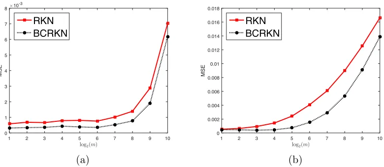
and thus could be advantageous in practice. We show this by an illustrative example used in Zhang et al. (2015). Consider the model f∗(x) = min{x,1−x} with x∼Uniform[0,1] and the noise ∼N(0, σ2) with σ2 = 15. Let K(x, t) = 1 + min{x, t}. Then f∗ ∈ HK
and kf∗kK = 1.We first compare the distributed RKN and the distributed BCRKN when
λ=|D|−2/3, a theoretically optimal choice. We generate|D|= 4098 sample points and use
number of partitions m ∈ {2,4,8,16,32,64,128,256,512,1024}. The mean squared errors of two methods are plotted in Figure 1 (a). We see BCRKN slightly outperforms RKN for all m.
Recall that the analyses in Zhang et al. (2015); Lin et al. (2017) and this paper indicate the optimal choice of the regularization parameter isλ=|D|−θ withθan index depending on the regularity of the true target function f∗ and the effective dimension of the integral operatorLK. Clearly both are unknown in practice and thus a theoretical optimal choice
of the regularization parameter is actually not available. At the same time, in a big data setting where distributed regression is necessary globally tuning the optimal parameter is either impossible or too time consuming. A reasonable way is to tune the parameter locally to get optimal choice λi =|Di|−θ on Di and then underregularize it using
λ=λ log|D|
log|Di|
i =|D|
−θ.
So we next compare the use of RKN and BCRKN in distributed regression when this pa-rameter selection strategy is used. The results are shown in Figure 1 (b). We see the requirement on the number of local processors becomes more restrictive for both methods, indicating that underregularizing locally optimal parameter does not lead to globally opti-mal parameter. BCRKN significantly outperforms RKN asmincreases, indicating it is less sensitive to the parameter selection when a globally optimal parameter is not available.
1 2 3 4 5 6 7 8 9 10 log2(m)
0 1 2 3 4 5 6 7 8
MSE
×10-3
RKN BCRKN
1 2 3 4 5 6 7 8 9 10
log2(m)
0 0.002 0.004 0.006 0.008 0.01 0.012 0.014 0.016 0.018
MSE
RKN BCRKN
(a) (b)
Figure 1: MSE of distributed RKN and distributed BCRKN. (a)λ=|D|−2/3 is used. (b) λis first tuned locally and the underregularized.
Finally, it is worth mentioning that debiasing techniques have also been developed to improve the accuracy of statistical inference of distributed lasso and received considerable attention recently (B¨uhlmann, 2013; Zhang and Zhang, 2014; Javanmard and Montanari, 2014; Lee et al., 2017; Battey et al., 2015).
4. Preliminary lemmas
The following lemmas can be found in Lin et al. (2017); Guo et al. (2017a).
Lemma 7 Let D be a sample drawn independently according to ρ and g be a measurable
bounded function on Z and ξg be a random variable with values on HK given by ξg(z) =
g(z)Kx for z= (x, y)∈ Z.For any 0< δ <1,with confidence at least 1−δ, there holds
(λI+LK)−
1 2 1
|D|
X
z∈D
ξg(z)−E[ξg]
!
K
≤ kgk∞log
2
δ
κ B|D|,λ.
Lemma 8 LetDbe a sample drawn independently according toρ.If|y| ≤M almost surely,
then with confidence at least1−δ,there holds
(λI+LK)
−1 2( 1
|D|S ∗
DyD−LK,Df∗)
K ≤2MB|D|,λlog
2
δ.
Lemma 9 LetDbe a sample drawn independently according toρ.If|y| ≤M almost surely,
then for any 0< δ <1,with confidence at least 1−δ, there holds
ΞD :=k(λI+LK)−
1
2(LK−LK,D)k ≤ B|D|,λlog2
IfAandB are invertible operators on a Banach space, then by the second order operator decomposition proposed in Lin et al. (2017), we have
A−1−B−1 =B−1(B−A)B−1(B−A)A−1+B−1(B−A)B−1. (18) This implies the following decomposition of the operator product
BA−1= (B−A)B−1(B−A)A−1+ (B−A)B−1+I. (19) WithA=LK,D+λIandB=LK+λIin (19), and applying Lemma 9, we have the following
bound fork(LK+λI)(LK,D+λI)−1k; for the detailed proof see Guo et al. (2017a).
Proposition 10 For any 0< δ <1,with confidence at least 1−δ, there holds
ΩD :=k(LK+λI)(LK,D+λI)−1k ≤
B|D|,λlog2δ √
λ + 1
!2
.
Moreover, the confidence set is the same as that in Lemma 9.
Lemma 11 Let Q be positive random variable. If there are constants a > 0, b >0, τ >0
such that for any 0 < δ ≤1, with confident at least 1−δ, there holds Q ≤a(logbδ)τ,then
for anys >0 we have E[Qs]≤asbΓ(τ s+ 1).
Proof Note the condition implies that for all t >0 there is PrhQτ1 > t
i
≤bexp
− t
a1/τ
.
So we have
E[Qs] = E h
Q1/τ
τ si
=τ s
Z ∞
0
tτ s−1Pr
h
Qτ1 > t
i
dt
≤ τ sb
Z ∞
0
tτ s−1exp
− t
a1/τ
dt
= bτ sΓ(τ s)as=asbΓ(τ s+ 1).
This proves the lemma.
5. Error analysis of BCRKN in L2ρ
X when r≥
1 2
We will split the proof of Theorem 1 into three cases: 0< r < 12, 12 ≤r≤ 3 2, and
3
2 < r≤2.
In this section we prove it for the second and third cases while leave the first case to Section 7. Denote ∆D = |D|1 SD∗(yD−SDf∗).
Proposition 12 If 12 ≤r≤ 3
2, we have
kfD,λ] −f∗kL2
ρX ≤2ΩD
(λI+LK)
−1 2∆D
K+λ r(Ω
D)rku∗kL2
Proof By the triangle inequality, we have
f
] D,λ−f
∗ L2 ρX ≤ f ] D,λ−E
∗[f] D,λ] L2 ρX + E
∗[f] D,λ]−f
∗
L2
ρX
, (20)
where E∗[fD,λ] ] = (2λI+LK,D)(λI +LK,D)−2LK,Df∗ is the conditional expectation with
respect toyD given xD.
For the first term
f
]
D,λ−E∗[f ] D,λ] L2 ρX
, noting that 2λI+LK,D and (λI+LK,D)−1
commute, we have
f
] D,λ−E
∗
[fD,λ] ]
L2 ρX = L 1 2
K(2λI+LK,D)(λI+LK,D) −2∆
D K ≤
(λI+LK) 1
2(λI+LK,D)− 1 2
(λI+LK,D)
−1
2(2λI+LK,D)(λI+LK,D)− 1 2 ×
(λI+LK,D)
−1
2(λI+LK) 1 2
(λI+LK)
−1 2∆ K
≤ 2ΩD
(λI+LK)
−12∆ D
K, (21)
here we have used the fact (Blanchard and Kr¨amer, 2010) that
kAsBsk ≤ kABks, 0≤s≤1,
for positive operatorsA and B on Hilbert spaces.
For the second term, we have
E∗[fD,λ] ]−f∗= [(2λI+LK,D)(λI+LK,D)−2LK,D−I]f∗=λ2(λI+LK,D)−2f∗.
By the regularity condition (4),
E
∗
[fD,λ] ]−f∗
L2
ρX
= λ2(λI+LK,D)−2Lru∗
L2
ρX
≤ λ2
(λI+LK)
1
2(λI+LK,D)−2Lr− 1 2
K L
1 2u∗
K
≤ λ2
(λI+LK) 1
2(λI+LK,D)− 1 2
(λI+LK,D)−
3 2Lr−
1 2 K L 1 2u∗
K
≤ λ2(ΩD)
1 2
(λI+LK,D)−
3 2Lr−
1 2 K
ku∗kL2
ρX. (22)
Since 12 ≤r ≤ 3
2,we have
(λI+LK,D)−
3 2Lr−
1 2 K =
(λI+LK,D)r−2(λI+LK,D)−r+
1
2(λI+LK)r− 1
2(λI+LK)−r+ 1 2Lr−
≤ (λI+LK,D)r−2
(λI+LK,D)
−r+12(λI+L
K)r−
1 2
(λI+LK)−r+
1 2Lr−
1 2 K
≤ λr−2(ΩD)r−
1 2. Therefore, E ∗
[fD,λ] ]−f∗
L2
ρX
≤λr(ΩD)rku∗kL2
ρX. (23)
Then the conclusion follows by combining (21) and (23).
Proposition 13 If 32 < r≤2,we have kfD,λ] −f∗kL2
ρX ≤2ΩD
(λI+LK)
−1 2∆D
K+λΞD(ΩD)
3
2κ2r−3ku∗k
L2
ρX +λ
rΩ
Dku∗kL2
ρX.
Proof The proof is similar to Proposition 12. First,kfD,λ] −f∗kL2
ρX can be divided into two
terms by (20). The first term has been estimated in Proposition 12 as (21). We now focus
on the second term. To this end, by (22), we only need to estimate
(λI+LK,D)−
3 2L r−1 2 K .
When 32 ≤r <2,we have (λI+LK,D)−
3 2Lr−
1 2
K
= (λI+LK,D)−
1
2 (λI+LK,D)−1−(λI+LK)−1Lr− 1 2
K
+(λI+LK,D)−
1
2(λI+LK)−1Lr− 1 2
K
= (λI+LK,D)−
1
2(λI+LK)−1(LK−LK,D)(λI+LK,D)−1(λI+LK)(λI+LK)−1Lr− 1 2
K
+(λI+LK,D)−
1
2(λI+LK) 1
2(λI+LK)− 3 2Lr−
1 2
K .
By the bounds
(λI+LK,D)
−1 2 ≤ 1 √ λ,
(λI+LK)
−1 2 ≤ 1 √
λ,and kLKk ≤κ
2,we have,
(λI+LK,D)−
3 2Lr−
1 2 K ≤ 1 λ
(λI+LK)
−1
2(LK−LK,D)
(λI+LK,D)−1(λI+LK)
(λI+LK)−1L r−1 2 K +
(λI+LK,D)
−12(λI+L K) 1 2
(λI+LK)−
3 2Lr−
1 2 K
≤ λ−1ΩD
(λI+LK)
−1
2(LK−LK,D) κ
2r−3+λr−2(Ω
D)
1 2.
Therefore, putting the above bound back into (22) yields
E
∗[f] D,λ]−f
∗ L2 ρX ≤ λ
(λI+LK)
−12(L
K−LK,D)
(ΩD)
3
2κ2r−3ku∗kL2
ρX
+λrΩDku∗kL2
Now the conclusion follows by plugging (21) and (24) into (20).
Now we are ready to prove Theorem 1 and Corollary 2 for r≥ 12.
Proof of Theorem 1: Case 12 ≤r ≤ 2. By Lemma 8, we have with confidence at least 1−δ
2,
(λI+LK)
−12∆ D
K ≤2MB|D|,λlog
4
δ. (25)
By Lemma 9 and Proposition 10, we obtain that, with confidence at least 1− δ
2,
ΞD =k(λI+LK)−
1
2(LK−LK,D)k ≤ B|D|,λlog4
δ (26)
and
ΩD =k(LK+λI)(LK,D+λI)−1k ≤
B|D|,λlog4δ √
λ + 1
!2
(27)
hold simultaneously.
When 12 ≤r≤ 32,we apply (25) and (27) to Proposition 12 and obtain
kfD,λ] −f∗kL2
ρX ≤ 4M
B|D|,λlog4δ √
λ + 1
!2
B|D|,λlog4
δ +λ
r B|D|,λlog
4
δ √
λ + 1
!2r
ku∗kL2
ρX
≤ (4M +ku∗kL2
ρX)
B
|D|,λ √
λ + 1
3
(B|D|,λ+λr)
log4
δ
4
When 32 < r≤2,we apply (25), (26) and (27) to Proposition 13 and obtain
kfD,λ] −f∗kL2
ρX ≤ 4M
B|D|,λlog4δ
√
λ + 1
!2
B|D|,λlog4
δ
+λB|D|,λlog4
δ
B|D|,λlog4δ
√
λ + 1
!3
κ2r−3ku∗kL2
ρX
+λr B|D|,λlog 4
δ √
λ + 1
!2
ku∗kL2
ρX
≤ (4M+ 2κ2r−3ku∗kL2
ρX)
B
|D|,λ √
λ + 1
3
(B|D|,λ+λr)
log4
δ
4
.
So (7) is proved for all 12 ≤r ≤2.Applying Lemma 11 withb= 4,τ = 4, ands= 2, we obtain the desired estimation in (8).
Proof of Corollary 2 (ii). With 12 ≤r≤2 and the choice of λ=|D|−2r1+β,we have
B|D|,λ≤
2κ
p
|D|
(
κ|D|2(2r1+β) p
|D| +
p
C0|D|
β
2(2r+β) )
≤2κ
κ+pC0
and
B|D|,λ √
λ + 1≤2κ(κ+
p
C0)|D|−
r
2r+β|D|
1
2r+β + 1≤2κ
κ+pC0
+ 1. (29)
Then the conclusions follow from Theorem 1.
6. Error analysis in HK
In this section, we derive the error bound for kfD,λ] −f∗kK and prove the convergence of
BCRKN inHK.It is similar to the error analysis in L2ρX.
Proposition 14 If r∈[12,32],we have kfD,λ] −f∗kK ≤2λ−
1 2(ΩD)
1 2
(λI+LK)
−1 2∆D
K+λ r−1
2(ΩD)r− 1 2ku∗kL2
ρX.
If r ∈(32,2], we have
kfD,λ] −f∗kK ≤ 2λ−12(ΩD) 1 2
(λI+LK)
−1 2∆D
K+λ
1
2ΞDΩDκ2r−3ku∗k
L2
ρX
+λr−12ΩDku∗k
L2
ρX.
Proof By the triangle inequality in HK, we have
kfD,λ] −f∗kK ≤ kfD,λ] −E∗[fD,λ] ]kK+kE∗[fD,λ] ]−f∗kK.
To estimate the first term, we see that
fD,λ] −E∗[fD,λ] ] = (2λI+LK,D)(λI+LK,D)−2∆D.
Then
f
] D,λ−E
∗
[fD,λ] ]
K =k(2λI+LK,D)(λI+LK,D) −2∆
DkK
≤
(2λI+LK,D)(λI+LK,D)
−32
(λI+LK,D)
−12(λI+L K) 1 2
(λI+LK)
−12∆ D
K
≤ 2λ−12(ΩD) 1 2
(λI+LK)
−1 2∆D
K.
For the second term, we have
E
∗
[fD,λ] ]−f∗
K=
λ2(λI+LK,D)−2Lru∗
K ≤λ
2k(λI+L
K,D)−2L r−1
2
K kku ∗k
L2
ρX.
Following the same idea as in the proof of Proposition 12, we obtain forr ∈[12,32],
E
∗[f] D,λ]−f
∗
K
≤λr−12(ΩD)r− 1 2ku∗k
L2
ρX
and following the idea in the proof of Proposition 13, we obtain for r∈(32,2],
E
∗
[fD,λ] ]−f∗
K ≤λ
1
2ΞDΩDκ2r−3ku∗kL2
ρX +λ
r−1
2ΩDku∗kL2
The desired error bounds now follow by combining the estimates for both terms.
Proof of Theorem 3.Note that (25), (26) and (27) hold simultaneously with probability at least 1−δ.Therefore, when 12 ≤r≤ 32,we have with confidence at least 1−δ
kfD,λ] −f∗kK ≤ 2λ−
1 2
B|D|,λlog4δ
√
λ + 1
!
2MB|D|,λlog4
δ
+λr−12
B|D|,λlog4δ
√
λ + 1
!2r−1
ku∗kL2
ρX
≤ (4M+ku∗kL2
ρX)
B
|D|,λ √
λ + 1
2
(λ−12B|D|,λ+λr− 1 2)
log4
δ
3
and, when 32 < r≤2,
kfD,λ] −f∗kK ≤ 2λ−
1 2
B|D|,λlog4δ
√
λ + 1
!
2MB|D|,λlog
4
δ
+λ12B|D|,λlog4 δ
B|D|,λlog4δ
√
λ + 1
!2
κ2r−3ku∗kL2
ρX
+λr−12
B|D|,λlog4δ
√
λ + 1
!2
ku∗kL2
ρX
≤ 4M+ 2κ2r−3ku∗kL2
ρX
B|D|,λ
√
λ + 1
2
(λ−12B|D|,λ+λr− 1 2)
log4
δ
3
.
This proves the error bound (9). Then (10) follows from estimates (28) and (29), and (11) follows by applying Lemma 11.
7. Improve the error analysis by unlabelled data
The error analysis for the semi-supervised approach is more involved. Before we move on, notice that Theorem 1 with 0 < r < 12 is a special case of Theorem 4 with D0 = D when there is no unlabeled data. So upon finishing Theorem 4, we also obtain Theorem 1 with 0< r < 12.
We need to introduce an intermediate function. RecallLis a compact operator onL2ρ
X. Let {τi}∞i=1 and {ψi}∞i=1 be the eigenvalues and eigenfunctions of L. Then {ψi}∞i=1 form
an orthonormal basis of L2ρ
X. LetPλ be the projection operator on L
2
ρX that projects each
f ∈L2ρ
X onto the subspace spanned by {ψi :τi ≥λ},i.e.
Pλf =
X
{i:τi≥λ}
hψi, fiL2
ρXψi, ∀ f ∈L
2
By the isomorphism property (5) of L12,{φi =√τiψi :σi >0} form an orthonormal basis
of HK. Since {i : τi ≥ λ} is a finite set, it is obvious Pλf ∈ HK for all f ∈ L2ρX. Define
fλtr =Pλf∗.We can boundkfD]0,λ−f∗kL2
ρX as follows.
Proposition 15 We have
kfD]0,λ−f∗kL2
ρX ≤I1+I2+I3,
where
I1 =
(λI+LK) 1
2(2λI+LK,D0)(λI+LK,D0)−2
1
|D0|SD∗0yD0−LK,D0ftr
λ
K
I2 = λ
2(λI+L
K)
1
2(λI+LK,D0)−2ftr
λ
K,
I3 = kfλtr−f∗kL2
ρX.
Proof Note that
kfD]0,λ−f∗kL2
ρX ≤ kf
]
D0,λ−fλtrkL2
ρX +kf
tr
λ −f∗kL2
ρX. (30)
Since fD]0,λ−fλtr ∈ HK,by the isometry property (5) ofL
1 2 =L
1 2
K, we have
kfD]0,λ−fλtrkL2
ρX =kL
1 2
K(f ]
D0,λ−fλtr)kK≤ k(λI+LK)
1 2(f]
D0,λ−fλtr)kK. (31)
Recall that
fD]0,λ =fD0,λ+λ(λI+LK,D0)−1fD0,λ= (2λI+LK,D0)(λI+LK,D0)−2 1
|D0|S ∗ D0yD0. It is easy to check that
fD]0,λ−fλtr = (2λI+LK,D0)(λI+LK,D0)−2
1
|D0|S ∗
D0yD0−LK,D0ftr
λ
−λ2(λI+LK,D0)−2ftr
λ .
Putting this in (31) we have kfD]0,λ−fλtrkL2
ρX bounded by I1+I2. Together with (30), we
obtain the desired conclusion.
Next we estimate the three terms respectively. The third termI3 can be easily bounded
by the following lemma, which has been proved in Caponnetto (2006).
Lemma 16 We havekfλtr−f∗kL2
ρX ≤λ
rku∗k L2
ρX and kf
tr
λ kK ≤λ−
1
2+rku∗k
L2
ρX.
For the first term I1, we have the following bound.
Proposition 17 For any δ∈(0,1),with confidence at least 1−δ,there holds
I1 ≤
2M κ + 2ku
∗k L2
ρX
B|D0|,λ
√
λ + 1
3
B|D|,λ+λr
log4
δ
3
Proof Since 2λI+LK,D0 and (λI+LK,D0)−1 commute, we have
I1 =
(λI+LK)
1
2(2λI+LK,D0)(λI+LK,D0)−2
1
|D0|S ∗
D0yD0 −LK,D0fλtr
K ≤
(λI+LK) 1
2(λI+LK,D0)−
1 2
(2λI+LK,D0)(λI+LK,D0)−1
×
(λI+LK,D0)
−1
2(λI+LK) 1 2
(λI+LK)−
1 2
1
|D0|S ∗
D0yD0 −LK,D0fλtr
K
≤ 2ΩD0
(λI+LK)−
1 2
1
|D0|S ∗
D0yD0 −LK,D0fλtr
K .
Proposition 10 ensures that, with confidence at least 1−δ2,
ΩD0 ≤
B
|D0|,λ
√
λ + 1
2
log4
δ
2
. (32)
Now it suffices to consider the term
(λI+LK)
−12 1
|D0|SD∗0yD0 −LK,D0ftr
λ
K.We further
divide it into three parts as follows
(λI+LK)−
1 2
1
|D0|S ∗
D0yD0−LK,D0fλtr
≤
(λI+LK)−
1 2
1
|D0|S ∗
D0yD0−LKf∗
K +
(λI+LK)
−1
2(LKf∗−LKftr
λ ) K +
(λI+LK)
−12(L
K−LK,D0)fλtr
K.
By the definition ofyi0, it is easy to check that |D10|SD∗0yD0 = 1
|D|S ∗
DyD.Applying Lemma 7
withξg(z) =yKx, we obtain, with confidence at least 1−δ2,
(λI+LK)−
1 2
1
|D0|S ∗
D0yD0−LKf∗
K
≤ Mlog
4
δ
κ B|D|,λ.
By Lemma 16, we have
(λI+LK)
−1
2(LKf∗−LKftr
λ )
K
≤ kf∗−fλtrkL2
ρX ≤λ
rku∗k L2
ρX.
For
(λI+LK)
−1
2(LK−LK,D0)ftr
λ
K,observe that
(λI+LK)
−1
2(LK−LK,D0)fλtr
K ≤
(λI+LK)
−1
2(LK−LK,D0)
kf
tr λ kK.
By Lemma 16, we havekfλtrkK ≤λ−12+rku∗k
L2
ρX.By Lemma 9, we have with confidence at
least 1−δ
2,
(λI+LK)
−12(L
K−LK,D0)fλtr
K ≤λ
rB|D√0|,λ
λ ku
∗k L2
ρX log
4
with the confidence set the same as that for (32). Combining the above estimations together yields
(λI+LK)−
1 2
1
|D0|S ∗
D0yD0−LK,D0ftr
λ
K
≤
M κ +ku
∗k L2
ρX
B|D0|,λ
√
λ + 1
B|D|,λ+λrlog4
δ. (33)
Then our desired result follows by (32) and (33).
Proposition 18 For any δ∈(0,1),we have, with confidence at least 1−δ2, I2≤
B
|D0|,λ
√
λ + 1
λrku∗kL2
ρX log
4
δ
with the confidence set the same as that for (32).
Proof We have
I2 = kλ2(λI+LK)
1
2(λI+LK,D0)−2fλtrkK = λ2
(λI+LK) 1
2(λI+LK,D0)−
1
2(λI+LK,D0)−
3 2ftr
λ
K
≤ λ2k(λI+LK)
1
2(λI+LK,D0)−
1
2kk(λI+LK,D0)−
3 2kkftr
λ kK
≤ λr(ΩD0)
1 2ku∗kL2
ρX,
where we used the bounds k(λI+LK,D0)−
3
2k ≤λ− 3
2 and kftr
λ kK ≤λ r−1
2ku∗kL2
ρX.By (32),
we obtain the desired bound and confidence set.
Now we can prove Theorem 4.
Proof of Theorem 4.Plugging the bounds ofI1,I2,andI3into Proposition 15, we obtain
the error bound for kfD]0,λ−f∗kL2
ρX in (12).
If λ=|D|−2r1+β with 0< r≤ 1
2 and N(λ)≤C0λ
−β,we have
B|D|,λ≤
2κ
p
|D|
κ|D|−12|D| 1
2(2r+β) +pC 0|D|
β
2(2r+β)
≤2κ(κ+pC0)|D|−
r
2r+β.
Under the condition |D0| ≥ |D|21+r+ββ,we have
B|D0|,λ
√
λ =
2κ
p
|D0|λ
(
κ
p
|D0|λ+
p
N(λ)
)
≤ p2κ |D0||D|
1 2(2r+β)
κ|D0|−12|D| 1
2(2r+β) +pC 0|D|
β
≤ p2κ |D0||D|
1
2(2r+β)(κ+pC 0)|D|
β
2(2r+β)
≤2κ(κ+pC0).
Applying these two estimates to (12), we have for any δ ∈ (0,1), with confidence at least 1−δ,
kfD]0,λ−f∗kL2
ρX ≤C1|D|
− r
2r+β
log4
δ
3
where
C1 =
2M κ + 4ku
∗k L2
ρX
h
2κ(κ+pC0) + 1 i3h
2κ(κ+pC0) + 1 i
.
This completes the proof of Theorem 4.
Note we also proved Theorem 1 with 0< r < 12 because it is a special case of Theorem 4 withD0 =D. So we are in position to prove Corollary 2 (i).
Proof of Corollary 2 (i).When 0< r≤ 1
2, takeλ=|D|
−1+1β
.Then
B|D|,λ ≤
2κ
p
|D|
(
κ|D|2(1+1β) p
|D| +
p
C0|D|
β
2(1+β) )
≤ 2κ(κ+pC0)|D|
− 1
2(1+β) ≤2κ(κ+pC 0)|D|
− r
1+β
and
B|D|,λ √
λ ≤2κ(κ+
p
C0)|D|− 1 2(1+β)|D|
1
2(1+β) = 2κ(κ+pC 0).
Plugging them into the estimation (7) we obtain the desired learning rate.
8. Error analysis for distributed BCRKN
The following lemma is analogous to Guo et al. (2017a, Proposition 4).
Lemma 19 Let f]D,λ be defined by (14). We have
E
kf]D,λ−f∗k2L2
ρX
≤ m
X
j=1
|Dj|2 |D|2 E
kfD]
j,λ−f
∗k2
L2
ρX
+
m
X
j=1
|Dj| |D|
E[f
]
Dj,λ]−f
∗ 2
L2
ρX
. (34)
Proof of Theorem 5.By Theorem 1, for each fixed j∈ {1,2, . . . , m},
E
kfD]
j,λ−f
∗k2
L2
ρX
≤4Γ(9)C2
B
|Dj|,λ
√
λ + 1
6
B|Dj|,λ+λ
Then the first term on the right of (34) can be estimated as
m
X
j=1
|Dj|2 |D|2 E
kfD]
j,λ−f
∗k2
L2
ρX
≤4Γ(9)C2
m
X
j=1
|Dj|2 |D|2
B
|Dj|,λ
√
λ + 1
6
B|Dj|,λ+λ
r2. (35)
To estimate the second term on the right of (34), for each fixed j ∈ {1,2, . . . , m}, by Jensen’s inequality, we have
E[f
]
Dj,λ]−f
∗
L2
ρX
≤EhkE∗[fD]
j,λ]−f
∗k L2
ρX
i
.
We will bound the second term in two different ways according to the range of r. First consider the case when 12 ≤r ≤ 32.The bound (23) in the proof of Proposition 12 tells us that
E
∗[f]
Dj,λ]−f
∗
L2
ρX
≤λrΩrDjku∗kL2
ρX.
It follows that
kE[fD]
j,λ]−f
∗k L2
ρX ≤λ
rku∗k L2
ρXE
h
ΩrDj
i
. (36)
Applying Proposition 10 to each fixed j∈ {1, . . . , m}, with confidence at least 1−δ2, there holds
ΩDj ≤
B|Dj|,λlog
4
δ √
λ + 1
!2
≤
B
|Dj|,λ
√
λ + 1
2
log4
δ
2
.
By Lemma 11, this implies that for anys >0,
EhΩsDji≤2Γ(2s+ 1)
B
|Dj|,λ
√
λ + 1
2s
. (37)
Applying (37) with s=r to (36) yields
kE[fD]
j,λ]−f
∗k L2
ρX ≤2Γ(2r+ 1)ku
∗k L2
ρXλ
r
B
|Dj|,λ
√
λ + 1
2r
. (38)
Combining (34), (35) and (38), we have
E[kf]D,λ−f∗k2L2
ρX] ≤ 4Γ(9)C
2
m
X
j=1
|Dj|2 |D|2
B
|D√j|,λ
λ + 1
6
B|Dj|,λ+λ
r2
+4Γ2(2r+ 1)ku∗k2L2
ρXλ
2r m
X
j=1
|Dj| |D|
B
|Dj|,λ
√
λ + 1
4r
.
This proves the desired bound for 12 ≤r≤ 3 2.
For 32 < r≤2,by the bound (24) in the proof of Proposition 13, we have
kE∗[fD]
j,λ]−f
∗k L2
ρX ≤λΞDjΩ
3 2
Djκ
2r−3ku∗k L2
ρX +λ
rΩ Djku
∗k L2
So,
E[kE∗[fD]
j,λ]−f
∗k L2
ρX] ≤ λE
h
ΞDj(ΩD)
3 2 i
κ2r−3ku∗kL2
ρX +λ
rE[Ω Dj]ku
∗k L2
ρX
≤ λ
E
h
Ξ2Dj
i1 2
E h
Ω3Dj
i1 2
κ2r−3ku∗kL2
ρX +λ
rE[Ω Dj]ku
∗k L2
ρX.
From Lin et al. (2017, Lemma 17), we know
E
(λI+LK)
−1
2(LK−LK,D)
2
≤ κ
2N(λ)
|D|
and by (37) with s= 3,we have
E h
Ω3Dj
i
≤2Γ(7)
B
|D√j|,λ
λ + 1
6
.
Therefore,
kE[fD]
j,λ]−f
∗k2
L2
ρX
≤ 2λ2EhΞ2DjiEhΩ3Djiκ4r−6ku∗k2
L2
ρ
X
+ 2λ2r(E[ΩDj])
2ku∗k2
L2
ρ
X
≤ 2λ2κ 2N(λ)
|Dj|
2Γ(7)
B
|Dj|,λ
√
λ + 1
6
κ4r−6ku∗k2
L2
ρX
+32λ2rku∗k2L2
ρX
B
|Dj|,λ
√
λ + 1
4
≤ 4Γ(7)κ4r−4+ 32ku∗k2L2
ρX
B
|D√j|,λ
λ + 1
6
λ2N(λ)
|Dj|
+λ2r
. (39)
Combining (34), (35) and (39), we have
E[kf]D,λ−f∗k2L2
ρX]
≤ 4Γ(9)C2
m
X
j=1
|Dj|2 |D|2
B
|Dj|,λ
√
λ + 1
6
B|Dj|,λ+λ
r2
+ 4Γ(7)κ4r−4+ 32
ku∗k2L2
ρX
m
X
j=1
|Dj| |D|
B
|Dj|,λ
√
λ + 1
6
λ2N(λ)
|Dj|
+λ2r
.
This proves the conclusion for 32 < r≤2.
Next let us turn to the special case that the local machines are assigned the same number of observations, i.e.,|D1|=|D2|=· · ·=|Dm|.
Proof of Theorem 6. For 12 ≤ r ≤ 2, we choose λ = |D|−2r1+β. Then by the capacity
assumption (6), restriction on the number of local machinesm≤ |D|min{22rr−+β1,
2
fact|D1|=|D2|=. . .=|Dm|= |D|m,we have N(λ)
λ|Dj|
≤C0mN 1−2r
2r+β ≤C
0.
It follows that, for eachj = 1, . . . , m,
B|Dj|,λ √
λ =
2κ
p
λ|Dj|
(
κ
p
|Dj|λ
+pN(λ)
)
≤2κ(κ+pC0)
and
|Dj| |D|B
2
|Dj|,λ ≤8κ
2
κ2
|D||Dj|λ
+ N(λ)
|D|
≤8κ2(κ2+C0)|D|
− 2r
2r+β
and
λ2N(λ)
|Dj|
≤ C0|D|
− 2
2r+β|D| β
2r+βm
|D| ≤C0|D| − 2r
2r+β.
Then by Theorem 5,
E
kf]D,λ−f∗k2L2
ρX
≤C¯2κ(κ+pC0) + 1 6
16κ2(κ2+C0) +C0+ 1
|D|−2r2+rβ.
This completes the proof of Theorem 6.
Acknowledgments
The work described in this paper is partially supported by the National Natural Science Foundation of China (Grants No. 11401524, 11531013, 11571078, 11631015, 11671171). Lei Shi is also supported by the Joint Research Fund by National Natural Science Foundation of China and Research Grants Council of Hong Kong (Project No. 11461161006 and Project No. CityU 104012) and Zhuo Xue Program of Fudan University. Qiang Wu is also supported in part by the USDA National Institute of Food and Agriculture (Grant Number 2016-70001-24636). Part of the work was carried out while Zheng-Chu Guo was visiting Shanghai Key Laboratory for Contemporary Applied Mathematics. All authors contributed equally to this paper and are listed alphabetically. The corresponding author is Qiang Wu.
References
N. Aronszajn. Theory of reproducing kernels. Transactions of the American Mathematical
Society, 68:337–404, 1950.
H. Battey, J. Fan, H. Liu, J. Lu, and Z. Zhu. Distributed estimation and inference with statistical guarantees. 2015. arXiv preprint arXiv:1509.05457.
F. Bauer, S. Pereverzev, and L. Rosasco. On regularization algorithms in learning theory.
G. Blanchard and N. Kr¨amer. Optimal learning rates for kernel conjugate gradient regres-sion. In Advances in Neural Information Processing Systems, pages 226–234, 2010.
O. Bousquet and A. Elisseeff. Stability and generalization. Journal of Machine Learning
Research, 2:499–526, 2002.
P. B¨uhlmann. Statistical significance in high-dimensional linear models. Bernoulli, 19(4): 1212–1242, 2013.
A. Caponnetto. Optimal rates for regularization operators in learning theory. Technical re-port, MIT, 2006. http://cbcl.mit.edu/publications/ps/MIT-CSAIL-TR-2006-062.
pdf.
A. Caponnetto and E. De Vito. Optimal rates for the regularized least-squares algorithm.
Foundations of Computational Mathematics, 7(3):331–368, 2007.
E. De Vito, A. Caponnetto, and L. Rosasco. Model selection for regularized least-squares algorithm in learning theory. Foundations of Computational Mathematics, 5(1):59–85, 2005.
R. DeVore, G. Kerkyacharian, D. Picard, and V. Temlyakov. Mathematical methods for supervised learning. IMI Preprints, 22:1–51, 2004.
T. Evgeniou, M. Pontil, and T. Poggio. Regularization networks and support vector ma-chines. Advances in Computational Mathematics, 13:1–50, 2000.
X. Guo, J. Fan, and D.-X. Zhou. Sparsity and error analysis of empirical feature-based regularization schemes. Journal of Machine Learning Research, 17(1):3058–3091, 2016.
Z.-C. Guo, S.-B. Lin, and D.-X. Zhou. Learning theory of distributed spectral algorithms.
Inverse Problems, 33(7):074009, 2017a.
Z.-C. Guo, D.-H. Xiang, X. Guo, and D.-X. Zhou. Thresholded spectral algorithms for sparse approximations. Analysis and Applications, 15(3):433–455, 2017b.
L. Gy¨orfi, M. Kohler, A. Krzyzak, and H. Walk.A distribution-free theory of nonparametric
regression. Springer Science & Business Media, 2006.
A. Javanmard and A. Montanari. Confidence intervals and hypothesis testing for high-dimensional regression. Journal of Machine Learning Research, 15(1):2869–2909, 2014.
J. D. Lee, Q. Liu, Y. Sun, and J. E. Taylor. Communication-efficient sparse regression.
Journal of Machine Learning Research, 18(5):1–30, 2017.
S.-B. Lin, X. Guo, and D.-X. Zhou. Distributed learning with least square regularization.
Journal of Machine Learning Research, 18(92):1–31, 2017.
S. Smale and D. X. Zhou. Learning theory estimates via integral operators and their approximations. Constructive Approximation, 26:153–172, 2007.
I. Steinwart, D. R. Hush, and C. Scovel. Optimal rates for regularized least squares regres-sion. In Conference on Learning Theory, 2009.
H. Sun and Q. Wu. A note on application of integral operator in learning theory. Applied
and Computational Harmonic Analysis, 26(3):416–421, 2009.
V. Temlyakov. Approximation in learning theory.Constructive Approximation, 27(1):33–74, 2008.
G. Wahba. Spline models for observational data. SIAM, 1990.
Q. Wu. Bias corrected regularization kernel network and its applications. In International
Joint Conference on Neural Networks (IJCNN), pages 1072–1079, 2017.
Q. Wu, Y. Ying, and D.-X. Zhou. Learning rates of least-square regularized regression.
Foundations of Computational Mathematics, 6(2):171–192, 2006.
C.-H. Zhang and S. S. Zhang. Confidence intervals for low dimensional parameters in high dimensional linear models. Journal of the Royal Statistical Society: Series B (Statistical
Methodology), 76(1):217–242, 2014.
T. Zhang. Leave-one-out bounds for kernel methods.Neural Computation, 15(6):1397–1437, 2003.
Y. Zhang, J. Duchi, and M. Wainwright. Divide and conquer kernel ridge regression. In
Conference on Learning Theory, pages 592–617, 2013.
Y. Zhang, J. C. Duchi, and M. J. Wainwright. Divide and conquer kernel ridge regres-sion: a distributed algorithm with minimax optimal rates. Journal of Machine Learning