R E S E A R C H
Open Access
Numerical simulation for two-phase flow in a
porous medium
Souad Gasmi and Fatma Zohra Nouri
**Correspondence: [email protected] Mathematical Modeling and Numerical Simulation Laboratory LAM²SIN, Badji Mokhtar University, P.O. Box 12, Annaba, 23000, Algeria
Abstract
In this paper, we introduce a numerical study of the hydrocarbon system used for petroleum reservoir simulations. This system is a simplified model which describes a two-phase flow (oil and gas) with mass transfer in a porous medium, which leads to fluid compressibility. This kind of flow is modeled by a system of parabolic
degenerated non-linear convection-diffusion equations. Under certain hypotheses, such as the validity of Darcy?s law, incompressibility of the porous medium,
compressibility of the fluids, mass transfer between the oil and the gas, and negligible gravity, the global pressure formulation of Chavent (Mathematical Models and Finite Elements for Reservoir Simulation: Single Phase, Multiphase and Multicomponent Flows Through Porous Media, 1986) is formulated. This formulation allows the establishment of theoretical results on the existence and uniqueness of the solution (Gasmi and Nouri in Appl. Math. Sci. 7(42):2055-2064, 2013). Furthermore, different numerical schemes have been considered by many authors, among others we can refer the reader to (Chen in Finite element methods for the black oil model in
petroleum reservoirs, 1994; Chen in Reservoir Simulation: Mathematical Techniques in Oil Recovery, 2007) and (Gagneuxet al.in Rev. Mat. Univ. Complut. Madr. 2(1):119-148, 1989). Here we make use of a scheme based on the finite volume method and present numerical results for this simplified system.
Keywords: compressible fluids; porous medium; multiphasic flow; finite volume method
1 Introduction
The fluids flow within porous media has an important role in various domains, such as geothermal studies, geotechnics (the mechanics of soils), chemical engineering, ground water storage, hydrocarbon exploitation (see references [] and []),etc.In some cases, there are two or more fluids with different characteristics. We are concerned with the simulation of the displacement of a fluid by another one, within a porous medium, while the displacing fluid is immiscible with the fluid being displaced. Different numerical tech-niques, mainly based on finite elements, have been used by many authors to solve such problems, for example see [] and [].
In this paper we introduce a finite volume method for solving the hydrocarbon system model often used for petroleum reservoir simulations. To prevent consistency defects in the scheme, we propose to modify the mesh where the discontinuity occurs, because of the porous media. We propose to design our new scheme, called the ?diamond meshes scheme? (DMS), whose convergence is proved, and which can be used to solve the
ear discrete equations. Finally, numerical simulations confirm that the DMS is significantly useful for such difficult problems taking into account their physical properties.
In this case, there are only two chemical species, or components, gas and oil, where this last component may exist in both phases (gas and oil), that is to say, the heavy residual component in the oil phase and the light volatile component in the gas phase. In order to reduce confusion, we need to distinguish carefully between the ?oil component? and the ?oil phase?. This model, called a hydrocarbon system, is a simplified compositional model describing two-phase flow in a porous medium with mass interchange between them. Therefore it can predict compressibility and mass transfer effects, in the sense that it is assumed that there is mass transfer between the oil and the gas phase. In this model the ?oil component? (also called stock-tank oil) is the residual liquid at atmospheric pressure left after a differential vaporization, while the ?gas component? is the remaining fluid.
2 Mathematical model
One of the fluids wets the porous medium more than the other; we refer to this as the wetting phase fluid and we refer to the other as the non-wetting phase fluid. In an oil-gas system, oil is the wetting phase. Let us consider a bounded connex openofRd(d=
or ), describing the porous medium (the reservoir), with a Lipchitz boundary, and let tbe the time variabletin [,T[,T<∞. LetCGgbe the mass fraction of the gas component
in the gas phase, COg the mass fraction of the oil component (the light component) in
the gas phase, andCOothe mass fraction of the oil component (the heavy component) in
the oil phase which is equal to . While this distribution of the hydrocarbon components between the oil and gas phases plays an important role in a steam drive process, we cannot say that the mass of each phase is conserved because of the possibility of transfer of the oil component between the two phases. Instead, we observe that the total mass of each component must be conserved.
Then the mass flux of the oil and the gas components are
COgρgUg+ρoUo,
CGgρgUg.
The oil and gas mass components are
φ(COgρgSg+ρoSo),
φCGgρgSg.
Then, for each fluid, we can write the conservation equations as
∂ ∂t
φ(COgρgSg+ρoSo)
+∇ ·(COgρgUg+ρoUo) = ,
∂ ∂t
φ(CGgρgSg)
+∇ ·(CGgρgUg) = ,
()
where (i=o,g)Si,Ui,ρirepresent the saturation, the velocity, and the density of the phasei,
respectively. The parameterφis the porosity of the medium. We have
ρg=f(Pg,CGg),
ρo=f(Po),
wherePoandPg are the oil and gaz pressure respectively.
We consider compressible fluids, with constant dynamic viscosities and where the grav-ity effect is neglected. Under these hypotheses, Darcy?s law combined with the mass con-servation equations for each one of the component leads to the following system of partial differential equations of parabolic convection-diffusion type:
φ(x)∂ ∂t
ρgSg+ρoωloSo
+∇ ·ρgUg+ρoωolUo
= , ()
φ(x)∂ ∂t
ρoωhoSo
+∇ ·ρoωhoUo
= , ()
Uo= –K(x)
kro
μo
∇Po, ()
Ug= –K(x)
krg
μg∇
Pg, ()
where (i=o,g)Pi,μi,krirepresent the pressure, the viscosity, and the relative permeability
of the phasei, respectively. The parameterKis the absolute permeability of the medium andωc
o,c=h,lis the mass fraction of the componentc, denoted byhfor the heavy
com-ponent and bylfor the light component in the oil phase. We have
μg=f(Pg,CGg),
μo=f(Po),
krg=f(Sg,So),
kro=f(Sg,So).
Furthermore, we shall use the subscriptSto indicate standard conditions,i.e.appropriate conditions for the temperature and the pressure of medium.
LetρOS,ρGSbe the density (measured at standard conditions) of the oil and the gas
com-ponents, respectively. The gas formation volume factor, denoted byBG, is the ratio of the
volume of free gas (all of which is gas component), measured at the reservoir conditions, to the volume of the same gas measured at standard conditions. Thus
BG(P,T) =
VG(P,T)
VGS
.
LetWGbe the weight of free gas, sinceVG=WρgG andVGS=
WG
ρgS, then
BG=
ρgS
ρg
,
so that the volatility of the oil in the gas is expressed by the ratio
RV=
VOS
VGS
The mass fractions of the two components in the gas phase are
COg=
RVρoS
BGρg
,
CGg=
ρgS
BGρg
.
By adding the last two equations and noting thatCGg+COg= , we obtain
ρg=
(ρGS+RVρOS)
BG
.
The substitution of these mass fractions and densities into () gives, for the gas and the oil components,
∂ ∂t
φ
RV
BG
ρoSSg+ρoSo +∇ ·
RV
BG
ρoSUg+ρoUo
= ,
∂ ∂t
φ
ρgSSg
BG
+∇ ·
ρgSUg
BG
= .
()
We suppose that it is a saturated regime and is expressed by
So+Sg= . ()
The capillary pressure is given by
Pg–Po=Pc(So) =pc(So)pcM, ()
where
pcM=supPc(So) and ≤pc(So)≤. ()
We define the mobility of each phase by the formula
λi=
kri
μi
, i=o,g, ()
and the total mobilityλby
λ=λo+λg. ()
To simplify, we set
ρoh=ρoωoh, ()
ρ=ρg+ρo, ()
b=ρgλg+ρoλo, ()
Let us now introduce the new unknowns, namely the reduced saturation and the global pressure in the following way: if we denote bySi,mandSi,M, the residual and the maximum
saturations of the fluidi=o,g, respectively; the reduced saturation is given by
S= So–So,m –Sg,m–So,m
, ()
≤S≤. ()
The ?global pressure? was first introduced by Chavent and Jaffre [] in the following form:
P=
(Pg+Po) +γ(S), ()
with
γ(S) =
S
So,m
λg–λo
λ p
c(ξ)pcMdξ. ()
Hence
γ(S) =
S
α(ξ)dξ, ()
where
α(S) =λg(S) –λo(S) λ(S) p
c(S)PcM ()
is the capillary diffusion. Therefore, our model is given by the following simplified system:
(x)∂ ∂t
ρohS+φ(x)So,m
∂ ∂t
ρoh
–∇ ·K(x)ρohλo(S)∇P
+∇ ·K(x)ρohα(S)∇(S)= , ()
(x)∂
∂t(ρS) +φ(x) ∂
∂t(ρSo,m+ρg)
–∇ ·K(x)b(S,P)∇P+∇ ·K(x)d(P)α(S)∇S= , ()
λ(S)∇P·η= , α(S)∇S= , on×(,T), ()
S(x, ) =S(x), P(x, ) =P(x), in, ()
whereφ(x) =ϕ(x)( –So,m–So,g).
3 Weak formulations
First we introduce the following spaces:
H(div,) =v∈L, (,T)d,div(v)∈L, (,T),d= , , ()
V() =v∈H(div,),v·η= on,
W() =v∈V(),v(x,T) = in.
The weak formulation of problem ()-() is written as
(x)ρohS,∂v ∂t
–K(x)ρohλo(S)∇P,∇v
+
K(x)ρohα(S)∇S,∇v= (f,v), ()
(x)ρS,∂v ∂t
–K(x)b(S,P)∇P,∇v+K(x)d(P)α(S)∇S,∇v= (f,v), ()
where (·,·)is the inner product defined onW(). A theoretical study of the existence and uniqueness of the weak solution was done and the details of the results can be found in [].
4 Finite volume approximation
In this section we study the approximation of solutions to our model in the discrete finite volume framework. This family of schemes allows very general meshes and deals with the main properties of the physical features of the treated problems. The time interval [,T[ is divided into finite sub-intervals [tn,tn+[ of lengthtn,n= , . . . ,Mwitht= andtM=T.
The space domain (the reservoir) is discretized by a non-structured stitchingTh.
4.1 Notations
We introduce the following notation:
- Let|K|denote the cellKsurface,N(K)the set of triangles having a common side with
the cellK.
- LeteK,Lbe the common side of the trianglesKandLand→–ηK,Lbe the normal oriented
fromKtowardsL.
-→–ηeiis the external normal corresponding to the part ofeiat the boundary.
- LetShbe the set of sides of the stitchingThandS∗hbe the set of the interior sides.
- For a given sidee, let us denote bySandNthe extremitiese, byW andEthe two
triangles wheree=W¯ ∩ ¯E; byχethe diamond cell associated withegiven by
connecting the centers of gravities of the cellsW andEwith the extremitiesNandS
ofe.
- ((εi)i=,)are the four segments forming the border ofχe.
-→–ηε=|ε
i|(μxi,μyi)is the normal onεioutgoing ofχe.
- For a given node,V(N)is the set of triangles with this node in common.
For the numerical resolution of problem ()-(), the first two equations will be dis-cretized separately. For more details on finite volume methods, see for example [] and [].
4.2 Discretization of the first equation
LetCbe a cell of the stitchingTh, at timetn; we integrate () onCto get
t
C
(x)ρoh,nSn+–Sndx
+ t
C
(x)ρoh,nSnPn+–Pndx
+ t
C
φ(x)So,m
ρho,nPn+–Pndx
–
D∈N(C)
eCD
K(x)ρoh,nλno(S)∇Pnηe
+
D∈N(C)
eCD
K(x)ρho,nαn(S)∇Snηe
dx
= . ()
Therefore we obtain
|C| tCρ
h,n o,C
SnC+–SnC
+|C| tC
ρoh,,CnSn
C
Pn+
C –PnC
+|C| tφCSo,m
ρoh,,CnPCn+–PCn
–
D∈N(C)
eCD
Kρoh,nλno(S)∇Pnηe
dx
+
D∈N(C)
eCD
Kρoh,nαn(S)∇Snηe
dx
= . ()
This implies that
|C| tCρ
h,n o,CSnC++
|C| t
ρoh,,CnCSCn+φCSo,m
PCn+
= –|C| tCρ
h,n o,CSnC–
|C| t
ρoh,,CnCSnC–φCSo,m
PnC
+
D∈N(C)
Fn C,e–
D∈N(C)
Fn
D,e, ()
where (ρoh,,Cn)is the space derivative of (ρoh,,Cn), andFCn,eandFDn,eare the numerical flows of convection and diffusion, which are approximated by
FCn,e=Keρoh,e,nλno,e∇ePn|e|, ()
FDn,e=Keρoh,,enαne∇eSn|e|, ()
whereeis a side of the stitching, –→ηeis the normal ofeoutgoing fromC;Ke,ρoh,,en, andλno,e
denote the interpolations oneof the functionsK,ρh
o, andλo, respectively, while∇ePnis
the approximation of the gradient of the pressure on the sidee. The construction of the approached gradient oneis done by the so-called Green-Gauss method. It consists of ap-proaching the gradient by its means on a co-volume in the form of a diamond constructed around the sidee. We write
ρoh,,enλno,e=ρohPneλo
Sne, ()
ρoh,,enαne =ρohPneαSen, ()
and
∇eP=
|χe|
ε∈∂χe
whereχeis the diamond cell associated withe, andN(ε) andN(ε) are the extremities
ofε, one of the four segments forming∂χe(the boundary ofχe) and –→ηeis the unit normal
vector. The values ofPat the centersWandEarePWandPE, while the values at nodesN
andSare interpolated on the boundary and denoted byPN andPS. For convenience, we
omit the indicationη. Hence at each nodeNwe have
PN=
K∈V(N)
yK(N)PK, ()
whereV(N) is the set of triangles sharing the nodeN,PKis the value ofPat the center of
the cellKandyK(N) are the interpolation weights. The gradient of the saturation is given
by
∇eS=
|χe|
ε∈∂χe
(SN(ε)+SN(ε))|ε|
–
→η
e, ()
with
SN=
K∈V(N)
yK(N)SK. ()
4.3 Discretization of the second equation In the same way, integration of () implies
|C| tCρ
n CSnC++
|C| t
C
ρCh,nSnC+φC
ρhC,nSo,m+φC
ρCh,nPnC+
= –|C| tCρ
n CSCn–
|C| t
C(ρoh,,Cn)SnC–φC(ρoh,,Cn)So,m+φC(ρoh,,Cn)
PnC
+
D∈N(C)
GnC,e–
D∈N(C)
GnD,e, ()
whereGnC,eandGnD,eare the numerical flows of the convection and diffusion approximated by
GnC,e=Keben∇ePn|e|, ()
GnD,e=Kedenαen∇eSn, ()
with
bne=bneSne,Pne, ()
denαen=dnePneαSen, ()
whereeis a side of the stitching that limits the cellC,∇ePnis given by () and (), and
5 Numerical experiments
The problem given in ()-() was said not to be typical of a hydrocarbon system simu-lation, but it can be designed to test the resolution capabilities of the numerical method for problems involving sharp fronts.
The numerical tests are done on a homogeneousisotropicreservoir. The physical set-ting in -D was as follows. A horizontal rectangular reservoir= ], [×], [, dis-cretized with a structured mesh made up of , cells, with an intrinsic permeability of . was initially filled with a mixture of gas and oil, their residual saturations are . and ., respectively. The initial fluid (oil) distribution was taken to be uniform on the whole reservoir surface, and it had an associated initial pressureP= , bar. The
porosity is= .. The mobilities and the capillary pressure are given byPc= (s– )/,
λo= .,λg = ., andμw= , andμo= , the time step ist= s. These tests were
carried out using the free and open-source simulator for flow and transport processes in porous media, based on the Distributed and Unified Numerics Environment DUNE (see www.dumux.org).
5.1 Results and discussion
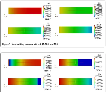
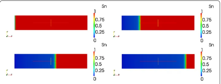
The numerical results shown in Figures - give the pressure for the wetting and non-wetting fluid, and the saturation for the non-non-wetting one. Because of the complexity of the problem, we have introduced new unknowns, namely the global pressure and the reduced saturation, in order to reduce the number of unknowns from six to two (for more details
Figure 1 Non-wetting pressure att= 0, 50, 100, and 175.
Figure 3 Non-wetting pressure att= 0, 50, 100, and 175.
see []). An explicit non-structured finite volume scheme has been used to solve this sim-plified problem with the new unknowns, and because of the non-structured meshes, we proposed a method based on ?diamond cells? to approximate the gradient. These results show that the scheme is very stable.
6 Conclusion
In this paper we proposed a new scheme based on the finite volume method for solving the displacement of a fluid by another one, within a porous medium, while the displac-ing fluid is immiscible with the fluid bedisplac-ing displaced. This gives the hydrocarbon system model often used for petroleum reservoir simulations. To prevent consistency defects in the scheme, we suggested to modify the mesh where the discontinuity occurs, because of the porous media. This convergent scheme, called the ?diamond meshes scheme? (DMS) was designed, to solve the associated nonlinear discrete equations. Finally, the numerical results, which are linked to our theoretical ones in [], confirm that the DMS is signifi-cantly useful for such difficult problems (see Figures -).
Competing interests
The authors declare that they have no competing interests.
Authors? contributions
All authors contributed equally to the writing of this paper. All authors read and approved the final manuscript.
Acknowledgements
This work was financially supported by the national research project (PNR08/23/997, 2011-2013). The authors are very grateful to the referees for their valuable and helpful comments, remarks and suggestions.
Received: 26 August 2014 Accepted: 1 December 2014
References
1. Chavent, G, Jaffre, J: Mathematical Models and Finite Elements for Reservoir Simulation: Single Phase, Multiphase and Multicomponent Flows Through Porous Media, pp. 1-40. Elsevier, Amsterdam (1986)
2. Gagneux, G, Lefevere, A-M, Madaune-Tort, M: Analyse mathématique de modèles variationnels en simulation pétrolière: le cas du modèle black-oil pseudo-compositionnel standard isotherme. Rev. Mat. Univ. Complut. Madr.2(1), 119-148 (1989)
3. Chen, Z: Finite element methods for the black oil model in petroleum reservoirs, pp. 1-28. I.M.A. Preprint Series #1238 (1994)
4. Chen, Z: Reservoir Simulation: Mathematical Techniques in Oil Recovery. SIAM, Philadelphia (2007)
5. Gasmi, S, Nouri, FZ: A study of a bi-phasic flow problem in porous media. Appl. Math. Sci.7(42), 2055-2064 (2013) 6. Afif, M, Amaziane, B: On convergence of finite volume schemes for one-dimensional two-phase flow in porous media.
J. Comput. Appl. Math.145, 31-48 (2002)