University of Trento
Department of MathematicsDoctoral School - XXX cycle
Ph.D. Thesis
Optimal choices:
mean field games with controlled jumps and
optimality in a stochastic volatility model
Advisor:
Prof.
Luca Di Persio
(University of Verona)
Optimal choices:
mean field games with controlled jumps and
optimality in a stochastic volatility model
Chiara Benazzoli
Trento, Italy June 6, 2018
Assessment Committee
Luca Di Persio University of Verona Advisor
Markus Fischer University of Padua Referee and Examiner
The sun came up with no conclusion Flowers sleeping in their beds This city’s cemetery’s humming I’m wide-awake, it’s morning
Road to Joy
Contents
Thesis Overview iv
I A class of mean field games with state dynamics governed by
jump-diffusion processes with controlled jumps 1
1 A class of mean field games with controlled jumps in the state
dynam-ics 2
1.1 The n-player gameGn . . . 4
1.2 The limiting gameG∞ . . . 8
2 Existence of a solution for the mean field game G∞ 12 2.1 The relaxed MFG problem G∞ . . . 12
2.1.1 Notation . . . 14
2.1.2 Assumptions . . . 15
2.1.3 Relaxed controls and admissible laws . . . 16
2.1.4 Relaxed mean-field game solutions . . . 18
2.2 Existence of a relaxed MFG solution . . . 20
2.2.1 The bounded case . . . 20
2.2.2 The unbounded case . . . 28
2.2.3 Technical results . . . 32
2.3 Existence of a relaxed Markovian MFG solution . . . 36
3 Existence of an ε-Nash equilibrium for the game Gn 38 3.1 Notation and Assumptions . . . 38
3.2 Markovian ε-Nash equilibrium . . . 40
3.2.1 L2-estimates for the state processes and the empirical mean inGn 42 3.2.2 Approximation results . . . 44
4 An illiquid interbank market model 51 4.1 The n-bank case . . . 51
Contents iii
4.2 The limiting game . . . 57
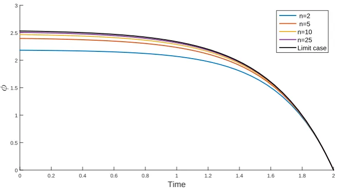
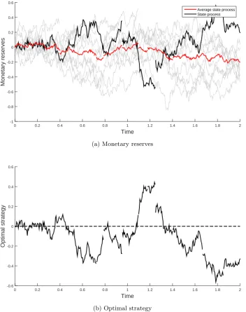
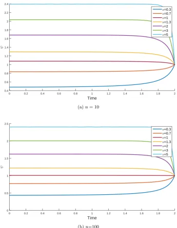
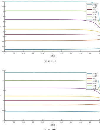
4.3 Simulations . . . 60
II An optimal control approach to stochastic volatility models 66 5 Stochastic optimal control theory 67 5.1 Stochastic optimal control problems . . . 67
5.2 The Hamilton-Jacobi-Bellman equation . . . 68
5.2.1 The verification Theorem . . . 71
5.2.2 Weak generalized solutions . . . 72
6 Optimality in a controlled Heston model 73 6.1 The Heston model . . . 73
6.2 The controlled Heston model . . . 75
6.3 The dynamic programming equation . . . 80
6.3.1 Semigroup approach . . . 87
6.4 A sub-optimal feedback control . . . 89
Thesis Overview
“So, what should I do?” is the big question this thesis is concerned with. Indeed, this is the query each player asks himself when in the middle of a game he has to make his move, as in Part I. And then, again, this is the question that one needs to answer inPart II when considering a stochastic optimal control problem in the framework of stochastic volatility modeling.
Part I. A class of mean field games with state dynamics governed by jump-diffusion processes with controlled jumps
In a nutshell, game theory studies the behaviour of a bunch of decision makers, called players or agents, when interacting in strategic situations. This means that the outcome of this interaction, which may be different for every participant, depends not only on one’s individual choices but also on the decisions taken by the other players. This connection ties together all the players, meaning that each agent cannot choose the strategy which maximises its preferences without considering the choices made by the others. Initially formalized by Von Neumann and Morgenstern in [VNM], over the past seven decades game theory results have been deeply and widely applied and extended to represent different situations in countless contexts. And the reason is straightforward since, associal animals, human beings are required to confront themselves into strategic decisions on a daily basis.
The distinctive trait of the class of non-cooperative, symmetric games with mean-field interactions we focus on is the fact that the state evolution of any player is given by a jump-diffusion process, where the size of the jumps is controlled by the player itself. Mean-field interaction refers to the fact that, by construction, both the dynamics of the private state and the possible outcomes of each player depend on the opposing players only through their overall distribution. This class of games is presented in
Chapter 1. Considering non-cooperative games, the aim is to discuss the existence of a Nash equilibrium for them, and possibly to compute it. A Nash equilibrium, firstly introduced by Nash in [Nas+50; Nas51], is a set of strategies, one for each player, that are optimal for each of them when they are simultaneously played. In other words, none of the players has an incentive to unilaterally deviate from it, since no other strategy can improve his outcome if the strategies of the others remain unchanged. Unfortunately, this
v
in general. However, since the games studied here are symmetric and charachterised by an interaction of mean-field type, it is possible to overcome (some of) these issues by considering their limiting game, that is the game arising when the number of players grows to infinity, which is in general easier to study. This is the main subject of the mean-field game theory, introduced by Lasry and Lions in [LL06a; LL06b; LL07] and, independently, by Huang, Malham´e, and Caines in [HMC06] combining ideas from the interacting particle system theory and results from the game theory. The key idea is that when the number of the intervening (homogeneous) players is large enough, the impact of one particular individual becomes morally negligible compared to the impact due to the overall population, and therefore it is possible to develop an efficient decision-rule by paying particular attention on the aggregate behaviour rather than on each individual player’s choice. Chapter 2 studies the existence of a mean-field game solution for the class of games introduced in the previous chapter by means ofrelaxed controls, introduced by Lacker in [Lac15a] and, independently, by Fischer in [Fis+17]. A mean-field game solution of the limiting game provides useful information also regarding the finite-player games and indeed it can be exploited to compute an approximate Nash equilibrium for them, at least when the number of agents is big enough, as examined inChapter 3.
Lastly, Chapter 4 presents a possible economic application of the class of games previously introduced: financial institutions, that are the players of this game, interact on an interbank lending market, aiming at controlling their level of reserves to balance their investment portfolio and, at the same time, to meet regulatory requirements. Assuming that this market is illiquid, each bank can access to it and therefore adjust its reserve level by borrowing or lending money only at some exogenously given instants, modeled as jump times of a Poisson process with constant intensity, which in turn represents a health indicator of the whole system.
Part II. An optimal control approach to stochastic volatility models
Stochastic control theory concerns dynamical systems whose evolution is modeled by stochastic differential equations depending on a control input which is chosen to reach the best possible outcome. Chapter 5 presents a (very short) introduction to stochastic optimal control theory in the case of continuous-time Markov diffusion pro-cesses, collecting well-known results which are used in the subsequent chapter. If the deterministic case has been a classical topic since the 1600s, optimal control in stochas-tic systems is a more recent theory: introduced by Bellman in the mid ‘50s in [Bel58], it has been widely applied in finance since the late ‘60s, when Merton formulated his portfolio-consumption model in [Mer69; Mer75] and then Black and Scholes presented their mathematical model, which bears their names, representing a financial market con-taining derivative instruments and leading to determine the fair price of a European call option. Starting from this single query, the results in stochastic optimal control were used to solve several problems and to answer to disparate questions in different economic fields.
vi
Part I
A class of mean field games with
state dynamics governed by
jump-diffusion processes with
Chapter 1
A class of mean field games with
controlled jumps in the state
dynamics
Every human being faces the surrounding world everyday by taking decisions and making choices based on their personal preferences and values. Being in asocial environ-ment, their behaviuors and their choices cannot ignore the social and cultural structure where they take place. Reservations in fancy hotels depend on the feedback read on review sites, the car one decides to buy is conditioned by advertising and by the car models driven by their neighbours, political preferences depend on the education one receives, on the discussions with the coworkers, on the opinion polls reported in the media and much more. We all are affected by the choices made by our families, by our friends and by our colleagues.
But at the same time, we write reviews about the hotels where we have stayed overnight, we zip around the city on our brand-new cars and we try to convince our office mates that our political opinion is, quite obviously, the right one. So, even if affected, we influence the choices made by our families, by our friends and by our colleagues as well.
Furthermore, one’s own behaviour and the one of other people influence not only the choices that every person makes, but also the outcomes of different situations one is in: which party will run the country after the next round of election? How much will the new Audi cost? Since, in principle, different people may have different wishes and preferences, the desired outcome may converge towards a same result or may diverge leading to a conflicting situation.
It would seem that as members of a economical, political and social life, each of us is actively playing a game whenever making a choice.
3
production knowing that the resulting aggregate supply, and therefore the resulting price, depends not only on his choice but also on the strategies adopted by its competitors. If the aim is to maximise one’s own gain, which is the proper level each producer has to choose?
Or, consider the consensus problem (as in [OSFM07], [Nou+13]). A group of people is required to agree on a final decision concerning a certain subject. Clearly, regarding one’s own preferences, each person would prefer an outcome rather than another ending and may try to convince the others of the goodness of its own beliefs. Then, the final agreement depends upon the preferences and the persuasive skills of all the people.
Decision-makers’ interaction is the main subject of game theory, and in particular
mean field game theorystudies a class of differential decision problems characterised by
a large (say huge, or better infinite) number of small and similar (say identical) players which are coupled together through their empirical average. Models with too many agents who mutually interact may be inefficient from a mathematical point of view, since it is not possible to consider simultaneously the dynamics of all the players, all their possible choices and all the ways these choices reflect on the other participants. Indeed, it would mean considering too many coupled equations and too many constraints at the same time, which may be not feasible. Actually, such a model would describe every detail of the reality, but it would be humanly and, even worse, computationally impossible to be solved. Therefore, the aim of mean field game theory is to simplify
a (specific) class of large population games to make them more tractable, but without losing their meaning. Somehow,mean field games look at the big picture.
Mean Field Games (MFGs, henceforth) were introduced by Lasry and Lions in [LL06a; LL06b; LL07] and, independently, by Huang, Malham´e, and Caines in [HMC06] combining ideas from the interacting particle system theory and results from the game theory. Interacting particles become here interacting decision makers, i.e. rational play-ers provided with preferences and goals who interact in a strategic situation, meaning that the outcome of the game for each of them depends on its own actions as well as on the strategies chosen by all the other players. Therefore, the behaviour of the peers becomes a crucial variable in computing one’s own optimal strategy. Then, considering again the analogy with an interacting particle system, the outcome of a game is not the
sum of the forcesas in a physics model, but it is the sum of rational choices made by the
players. In [GLL11], the authors strongly support that the primary purpose of MFGs is not (or not only) to compute and describe theinevitableresult of a strategic game but it is to explain why the inevitable emergent phenomenon is a natural response of coherent behaviours.
The purpose of this chapter is to introduce the class of MFGs we will study in the following. Section 1.1 presents Gn: a non cooperative, symmetric, n-player game with
1.1 The n-player gameGn 4
these games which guarantee the possibility of introducing the corresponding theoretical limiting game. This is the mean field game G∞ arising when the number of players n
grows to infinity, which is introduced in Section 1.2 along with the concept of mean field game solution.
1.1
The
n
-player game
G
nWe present here the n-player game Gn, a non cooperative, symmetric game with
mean-field coupling that is the main interest of the Part I of this Thesis.
LetT >0 be a fixed and finite time horizon and let (Ω,F,(Ft)t∈[0,T], P) be a filtered
probability space, supporting n independent Brownian motions Wi, for i = 1, . . . , n, andnindependent Poisson processes Ni, fori= 1, . . . , nwith the same time-dependent intensity functionν(t).The filtration (Ft)t∈[0,T]is assumed to satisfy theusual conditions,
meaning that it is complete, i.e. F0contains all theP-null sets, and it is right-continuous,
i.e.
Ft=
\
s>t
Fs for all t∈[0, T].
The state of each player i in the game, denoted by Xti,n and belonging to the real space, evolves in time accordingly to the following stochastic differential equation
dXti,n=b(t, Xti,n, µtn)dt+σ(t, Xti,n)dWti+β(t, Xt−i,n, µnt−, γit)dNeti, (1.1)
subjected to a given initial condition
X0i,n=ξi.
Here,Neti denotes the compensated Poisson processNeti =Neti− Rt
0ν(s)ds and µn stands
for the empirical measure of the systemXn= (X1,n, . . . , Xn,n), which is defined for any timet∈[0, T] as
µnt = 1
n
n
X
i=1
δXi,n
t , (1.2)
where δx denotes the Dirac delta measure at the point x. In addition we assume that
the initial conditions ξi, i = 1, . . . , n, are mutually independent real-valued random variables, all distributed according to the same distribution χ and that they are also independent from the noisesWi,Ni introduced before.
Observe that the functionsb,σ andβ appearing in the SDEs (1.1) do not depend on the specific playeri, meaning that they are equal for any agent even if computed relative to the different players’ positions/strategies.
Each playerihas the chance to control his position, or better the dynamics defining his state, by choosing at any time t ∈ [0, T] a control input γi
t. Each control process
γi = (γti)t∈[0,T], also called the strategy chosen by player i, takes values in the action
1.1 The n-player gameGn 5
definition of the SDE (1.1). This class of strategies is called the set of the admissible control processes and it is termedAi. We assume that the admissibility of a control does
not depend on which specific agent is going to play it, i.e. Ai =A for all i= 1, . . . , n.
Then, an admissible strategy profileγ for the gameGn, also called simply an admissible
strategy, is an n-tuple (γ1, . . . , γn) of admissible controls γi ∈ A for all i = 1, . . . , n, collecting the control processes chosen by each player.
Observe that strategies can be distinguished between open-loop strategies, if they depend only on the time variable, i.e. γi=γi(t), and feedback strategies, if the decision rule selects an action as a function also of the current state of the system x, i.e. γi =
γi(t, x). The more appropriate type depends on the context and in particular it is due to the information each player has: if any player has knowledge only of the initial state of the system and he cannot observe either the state of the system or the strategies chosen by the other players, it is natural to consider open-loop strategies, whereas, it is more suitable to consider feedback strategies if the players can observe the state of the system at any time.
Remark 1.1.1. In the following, we will require precise regularity conditions, both on the
dynamics (1.1) and on the admissible strategiesA, so as to guarantee the existence of a unique strong solution to the SDEs (1.1).
Compared to the setting introduced in [Lac15a], which is a key reference for this Part I, the dynamics of all players in this game are given by jump-diffusion processes rather than continuous-time diffusion processes. This provides greater flexibility in the modeling of the players’ dynamics.
In equation (1.1), the control of each player γi appears in the function β which multiplies the corresponding compensated Poisson ProcessNei, meaning that playerican
affect the magnitude of the jumps appearing in his dynamics whereas, as formulated, no control is set on when these jumps occur. Indeed, the intensity function of the Poisson processes,ν(t), which is the same for all players, is not influenced by any control.
Remark 1.1.2. It should be pointed out that a control component could be also applied
to the drift term b and to the diffusive component σ. This problem is already faced, and solved, in [Lac15a] and this is the main reason we skip it here. However, a more complete study is presented in [BCDP17a].
The dynamics of the nplayers are explicitly coupled together through the empirical distribution of their positions, µn. Although no strategy appears in the dynamics of
player i but its own, the whole strategy profile (γ1, . . . , γn) has an implicit impact on the dynamics Xi,n, i.e. Xi,n = Xi,n(γ). Indeed, Xi,n depends on the measure flow
µn = (µn
t)t∈[0,T], whose evolution is in turn affected by the choices made by all the
players in the game, since it depends on the state of all the agents. It will be relevant in the following observing that the empirical distribution is the only source of interaction among the evolution of the players’ states, since this is the only way Xj,n and γj may
1.1 The n-player gameGn 6
Each player takes part in the game in the hope of optimizing his outcome. The result of Gn relative to player iis given by the expected costJi,n, defined as
Ji,n=E
Z T
0
f(t, Xti,n, µnt, γti)dt+g(XTi,n, µnT)
, (1.3)
and therefore playeriaims to minimise it. As for the dynamics, also in the cost criterion, both the running cost functionf and the terminal cost functiong, which depend on the state and the strategy of the player and on the empirical distribution, are equal for each player, but then computed with respect to the different players’ positions/strategies. Furthermore, by its definition, the expected cost faced by playeri,Ji,n, depends on the opponents’ choices, i.e. Ji,n=Ji,n(γ1, . . . , γn), due to (and only through) the empirical measure µn.
As pointed out before, by construction, both the dynamics of the private state, given in equation (1.1), and the cost functions, in equation (1.3), of each player depend on the opposing players only through the distribution of all the participants,µn. This kind of coupling is said to be of mean-field type. Inter alia, mean field interaction implies that the dependence on the opponents is anonymous: for each agent it is irrelevant which other particular player chooses which specific control but he cares only about the resulting aggregate state position. In other words, considering player i, a permutation of the other players’ identities would lead unchanged the population distributionµn and
therefore would not modify the game from his point of view since both his dynamics and his cost functions are invariant under such a permutation.
As defined, Gnis a non cooperative game, meaning that each agent pursues his own
interest which in principle may conflict with the goals of the other players. In multi-person decision making problem, the meaning of optimality is not univocal, and in the following we will always consider Nash optimality.
Notation. Given an admissible strategy profileγ = (γ1, . . . , γn)∈ Anand any admissible
controlη∈ A, (η, γ−i) denotes a further admissible strategy where playerideviates from
γ by playingη, wheres all the other players continue playing γj,j6=i, i.e.
(η, γ−i) = (γ1, . . . , γi−1, η, γi+1, . . . , γn).
Then,
Definition 1.1.1. An admissible strategy profile γ = (γ1, . . . , γn)∈ An is a Nash
equi-librium of the n-player gameGn if for each i= 1, . . . , n and for any admissible strategy
η∈ A
Ji,n(η, γ−i)≥Ji,n(γ). (1.4)
1.1 The n-player gameGn 7
different admissible strategy. Indeed, considering anyi,γi is a best response of playeri
if his opponents play accordingly toγ, i.e.
γi = arg min
η∈AJ i,n(η, γ
−i)
and a unilateral change would lead to a higher (or at least not lower) expected cost. Sometimes, explicitly computing a Nash equilibrium of a game, or even proving its existence, is a too difficult task and therefore a slightly weaker equilibrium concept is introduced. Namely,
Definition 1.1.2. For a given ε≥0, an admissible strategy profile γ = (γ1, . . . , γn) ∈
An is an ε-Nash equilibrium of the n-player game G
n if for each i = 1, . . . , n and for
any admissible strategy η∈ A
Ji,n(η, γ−i)≥Ji,n(γ)−ε . (1.5)
Naturally, a Nash equilibrium of the game Gn is a0-Nash equilibrium.
In other words, a strategy profile (γ1, . . . , γn) is anε-Nash equilibrium if for each player in the game an unilateral change of his strategy when the others remain unchanged may lower the expected cost, but providing a maximum saving of ε.
Remark 1.1.3. In the two previous definitions, both Nash and ε-Nash equilibrium are
defined with respect to open loop strategies. Analogously, these definitions can also be rewritten considering feedback strategies, but a clarification is necessary. Let γi(t, x) be the feedback rule of player i6= 1 and consider what happen when player 1 deviates: since the state processes depend on the mean measure of the system, they depend on the control of the deviating player and then, even if the feedback function γi is kept fixed, the resulting strategy γi(t, Xti,n) differs form the one in the initial scenario, violating the Definitions 1.1.1 and 1.1.2. In this case a different notion of equilibrium may be consider, the so called feedback Nash equilibrium.
By its definition, searching for a Nash equilibrium means solving, simultaneously, n
optimization problems which are coupled together and, in turn, rely onndynamic state processes that are also coupled together. Then, the difficulty of such a task is clear. Moreover, the complexity of this problem becomes larger and larger as the number of players increases. However MFG theory is a powerful tool to investigate the existence of a (approximate) Nash equilibrium at least for particular symmetric games when the number of the intervening agents is pretty large and the impact of one particular indi-vidual may be negligible compared to the influence of the overall population. We briefly present the fundamental underlying idea of this theory in the following section.
A crucial characteristic of these games Gn, which will allow tractability for the
cor-responding limiting game and it is a common requirement in MFG theory, is their
symmetry. First, the population in the game is required to be of homogeneous players,
1.2 The limiting game G∞ 8
functions. This is our case since the functionsb,σandβappearing in the dynamics (1.1) and the cost functions f and g in equation (1.3) do not depend on the specific player, although then they are evaluated at the state of the related player. Second, as pointed out before, the interaction between the players is of mean-field type and therefore the opponents are anonymous since, for each player, a permutation of the other agents’ identity does not modify the game.
1.2
The limiting game
G
∞In a game with a small number of players the position, and thus the strategy, of one single agent can significantly affect the distribution of the state across the players,
µn, and therefore the outcome of the game. On the contrary, when the number of
in-tervening agents in a homogeneous population grows to infinity, the behaviour of just one single player becomes morally negligible in the aggregate. In this case, large popu-lation condition can be exploited to develop efficient decision-rules by paying particular attention on the population behaviour rather than on each individual player’s choice. See [HMC06]. Indeed, assuming that the population is distributed according to a given distribution, if the number of players is big enough, when a singular player deviates from his position in favor to a different one the population distribution does not move significantly. Therefore the deviation of just one player is not substantially felt by the other participants. This is the so called decoupling effect. Clearly, what has been said strongly depends on the fact that the interaction among the agents is of mean field type, otherwise this would not be true.
Therefore, in a symmetric game with a large homogeneous population and mean field interaction, it is possible to focus on just one representative player, say player p, and summarize the contribution of all his opponents through the population distribution, that is a measure flowµ= (µt)t∈[0,T], whereµtis a probability distribution over the state
space, in our caseµt∈ P(R). The crucial point is that, since (at least theoretically) the
impact of the choice of player p does not influence the population distribution, he can consider µ as a fixed deterministic function µ: [0, T] → P(R) when he searches for his
optimal control among all the possible admissible strategies.
In the following we consider the naive, theoretical generalization of the previous game
Gnto the the case when the number of players is infinite. We refer to this game asG∞.
Let (Ω,F,(Ft)t∈[0,T], P) be a filtered probability space satisfying the usual conditions,
supporting a Brownian motion W and a Poisson process N with intensity ν(t). The state of the representative player p,X= (Xt)t∈[0,T], moves accordingly to
dXt=b(t, Xt, µt)dt+σ(t, Xt)dWt+β(t, Xt−, µt−, γt)dNet, (1.6)
subjected to the initial condition
1.2 The limiting game G∞ 9
As before, assumptions granting the existence of a unique strong solution to the SDE (1.6) will be given in the following and for now we denote byAthe admissible strategies that player p can choose from. Since different choices for the control process γ leads to dif-ferent controlled dynamics, we will sometime stress this dependence by writingX(γ) or
Xγ to denote the solution to the SDE (1.6) under γ ∈ A.
The effectiveness of an admissible strategyγ is evaluated accordingly to the expected cost of the gameJ =J(γ), which is defined by
J =E
Z T
0
f(t, Xtγ, µt, γt)dt+g(XTγ, µT)
. (1.7)
The definition of the expected costJ is equal to the one in the gameGn. However, since
at this point the impact of the choice of player p no longer influences the population distribution being µ considered as fixed, then the outcome J depends directly only on the strategy γ chosen by the representative player p. Therefore, player p now faces a single-agent optimization problem and thus an admissible strategy ˆγ ∈ A is optimal if it attains the minimum of the expected cost, i.e.
J(ˆγ) = inf
γ∈AJ(γ).
Clearly, an optimal strategy ˆγ depends by definition on the population distribution µ
which is selected at the beginning. Therefore, it still depends on the choices of all the opponents that are summarised in this measure flowµ, but nevertheless, contrary to the previous case, they are kept fixed in this optimization step.
The subsequent step regards consistency for the choice of the measure flow µ that playerp considers when optimizing. In a nutshell, due to the symmetry of the pre-limit game Gn the statistical properties of the representative player should approximate the
empirical distribution generated by all the participants. Indeed, since all the infinite players in the game are identical (their dynamics solve the same SDE (1.6), their objec-tives matches and they interact symmetrically), being in the same situation, they would all act in the same way, meaning that they would all choose the same strategy. This means that an optimal strategy ˆγ for player p is optimal also for all the other players when they are in place ofp. Consequently, also the statistical distribution of the opti-mally controlled state Xˆγ would be the same for all the players, and therefore it must coincide with the population distribution, i.e.
L(Xˆγ) =µ . (1.8)
1.2 The limiting game G∞ 10
Definition 1.2.1. A mean field game solution for the gameG∞ is an admissible process
ˆ
γ ∈ A that is optimal, meaning that γˆ ∈ arg minγ∈AJ(γ), and, at the same time, it is
such that the related controlled dynamics Xγˆ satisfies the MFG consistency condition
µt=L(Xtγˆ) for allt∈[0, T].
A mean field game solution γˆ of G∞ is said to be Markovian if there exists a
mea-surable functionγˆ: [0, T]×R→A such that γˆt= ˆγ(t, Xt−).
So, a MFG solution represents anequilibrium relationshipbetween the individual strate-gies, required to be best responses to the infinite population behaviour, and the overall population distribution, required to be collectively determined by the players’ strategies. The existence of a mean field game solution for this game G∞is the main subject of
Chapter 2.
In Chapter 3 we look for an approximate Nash equilibrium for then-player gameGn,
for anynlarge enough. The construction of these equilibria will strongly depend on the existence of a (regular enough) MFG solution of the limiting game G∞. Indeed, there
are two different ways to justify why G∞ may be intended as the limit of the games
Gn and therefore why we refer to G∞ as limiting game: convergence or approximation
results. The latter refers to the fact that a Markovian MFG solution for G∞ may
allow to construct approximate Nash equilibria for the corresponding n-player games, at least if the number of players n is large enough. In particular, we will show that if there exists a Markovian MFG solution ˆγ = ˆγ(t, Xt−) for G∞, then the strategy
profile (ˆγ(t, Xt−1,n(ˆγ)), . . . ,γˆ(t, Xt−n,n(ˆγ))) is a εn-Nash equilibrium for the corresponding
game Gn, with the sequence εn satisfying εn → 0 as n → ∞. This approximation
result is also practically relevant since a direct verification of the existence of Nash equilibria for n-player games when nis very large is usually not feasible. Furthermore, the computation of these possible equilibria is not even numerically feasible, due to the curse of dimensionality. See, e.g., [HMC06], [KLY11], [CD13a], [CD13b], [CL15] as well as the recent book [Car16] for further details.
On the other hand, the key question in the convergence approach is if and in which sense a sequence of Nash equilibria for then-player gamesGnconverges towards a MFG
solution of a limiting game. Assuming that for each n the game Gn admits a Nash
equilibrium ˆγ = (ˆγ1, . . . ,ˆγn) then we expect that, at least heuristically, the empirical measure µn computed with respect to the optimally controlled processes Xi,n(ˆγ) con-verges to a deterministic measure flowµand that, in the light of the above observations, this measureµ coincides with the distribution of the optimally controlled stateXγˆ. In other words, a mean field game solution ˆγ for the gameG∞ should minimise
J =E
Z T
0
f(t, Xtγˆ,L(Xtˆγ),γˆt)dt+g(XTγˆ,L(X
ˆ
γ T))
,
subjected toXγˆ solving the McKean-Vlasov SDE
(
dXtˆγ=b(t, Xtγˆ,L(Xtˆγ)) +σ(t, Xtˆγ)dWt+β(t−, Xt−γˆ ,L(X
ˆ
γ
t−,γˆt−))dNet,
1.2 The limiting game G∞ 11
Chapter 2
Existence of a solution for the
mean field game
G
∞
In this chapter we study the stochastic differential game G∞ introduced in the
pre-vious Chapter 1. Section 2.1 briefly recalls the mean field game G∞, highlighting its
main characteristics and the main difficulties involved in its study. To overcome these issues, the previous game is modified and re-written from the perspective of the relaxed controls. Section 2.2 contains the main result of this chapter, that is the existence of a relaxed mean field game solution for G∞ whereas Section 2.3 investigates conditions
guaranteeing that a relaxed Markovian mean field game solution can be built.
The novel contributions of what presented here are contained in [BCDP17a]. The main reference for this chapter is [Lac15a].
2.1
The relaxed MFG problem
G
∞As introduced in Chapter 1, the MFGG∞we are interest in is the following. Fixed a
finite time horizonT >0, let (Ω,F,(Ft)t∈[0,T], P) be a filtered probability space, which
satisfies the usual conditions and supports a standard Brownian motionW and a Poisson processN with intensity functionν(t). These two processesW andN are assumed to be independent. The real-valued state variableX, which is controlled through the process
γ, i.e. X=Xγ, follows the dynamics
dXt=b(t, Xt, µt)dt+σ(t, Xt)dWt+β(t, Xt−, µt−, γt)dNet, t∈[0, T], (2.1)
with initial conditionX0 =ξ distributed according to a real-valued probability
distribu-tionχ∈ P(R). Here,µrepresents a measure flow, meaning thatµ: [0, T]→µt∈ P(R) is
a given deterministic function, whose precise meaning will be explained in what follows. An admissible control process, called also an admissible strategy, is any predictable control process γ = (γt)t∈[0,T] taking values in a fixed action space A⊂R and
2.1 The relaxed MFG problem G∞ 13
controls is denoted by A. Then, a control process is chosen in order to minimise the expected cost
J(γ) =E
Z T
0
f(t, Xt, µt, γt)dt+g(XT, µT)
,
and therefore ˆγ ∈ Ais said to be optimal if
J(ˆγ) = inf
γ∈AJ(γ). (2.2)
According to Definition 1.2.1, an optimal strategy ˆγ is a MFG solution for the game G∞
if the related controlled state ˆX =X(ˆγ) satisfies the MFG consistency condition (1.8), that isL( ˆXt) =µt for allt∈[0, T]. Our aim is to prove the existence of such a solution.
The own definition of mean field game solution, Definition 1.2.1, provides a (possible) constructive algorithmto build a solution for the MFG G∞. Indeed, this problem can
be solved by splitting it into two parts:
1. Optimization problem. Consider a fixed measure flow µand solve the stochastic minimisation problem infγ∈AJ(γ) finding the set of all the optimal strategies ˆγ =
ˆ
γ(µ), say ˆA(µ), which attain the minimum expected cost. Sinceµis treated as an exogenous parameter, it is non affected by the choice of the control strategy ˆγ. Clearly, the existence of an optimal control is not granted for free and existence analysis has to be developed;
2. Fixed point problem. Find, if there exists, a fixed point of the correspondence
Φ : µ7→ {L(Xtˆγ)t∈[0,T]: ˆγ ∈Aˆ(µ)}. (2.3)
If it exists, then the optimal control process γ∗ ∈ Aˆ(µ) which provides the fixed point conditionL(Xγ∗) =µis a MFG solution of the gameG∞.
Observe that, at least theoretically, the optimization problem in the previous step should be solved for any measure flowµ.
The main difficulty in the present approach is to show the existence of a fixed point for the mapping Φ. Indeed, classical results require the continuity of Φ, which is hard to prove. Lacker in [Lac15a] and, independently, Fischer in [Fis+17] introduce a new powerful approach, themartingale approach, to avoid the direct study of the regularity of the correspondence Φ by means of the so called relaxed controls. The basic idea is to re-define the state variable and the controls on a suitable canonical space supporting all the randomness sources involved in the SDE (2.1), and identify the solution to the MFG
G∞no longer with a stochastic process γ but with a probability measure P that can be
seen as the joint law of the control-state pair. Therefore, finding a relaxed solution to the MFG above will boil down to finding a fixed point for a different suitably defined set-valued map, easier to study.
2.1 The relaxed MFG problem G∞ 14
2.1.1 Notation
A real-valued function defined on the time interval [0, T],x: [0, T]→R, is said to be
c`adl`ag if it is continuous from the right at all t∈[0, T) and with finite left limit for all
t ∈(0, T]. The set of all real-valued c`adl`ag functions defined on [0, T] will be denoted by D=D([0, T];R). Then, it is well known that
Theorem 2.1.1. Each x∈D is a bounded, Borel measurable function with either finite or countably infinite discontinuities.
Proof. See, e.g., [Whi07].
This space D can be endowed with the Skorohod topology J1. Let Λ be the set of
strictly increasing functions ι: [0, T]→ [0, T] such that ι, along with its inverse ι−1, is continuous. Then for anyx, y∈D,J1-metric onD is defined by
dJ1(x, y) = inf
ι∈Λ{kx◦ι−yk∞∨ kι−Ik∞},
where I denotes the identity map. J1 denotes the topology induced by this metric. A
peculiar property of the Skorohod J1 topology is that whenever xn → x with respect
toJ1 then both the magnitudes and the locations of the jumps ofxn converge to those
of x. Moreover, the space (D, J1) is Polish. See [Whi07, Chapter 3-11-12] for further
details on the c`adl`ag space and the Skorohod topologyJ1.
Given any metric space (S, d), B(S) denotes the Borel σ-field of S induced by d. ThenP(S) stands for the set of all probability measures defined on the measurable space (S,B(S)). Furthermore, for any p≥ 1, Pp(S) ⊂ P(S) denotes the set all probabilities
onS such thatR
Sd(x, x0)
pP(dx)<∞for some (hence for all)x
0 ∈S. The spacePp(S)
will be endowed with the Wasserstein metric dW,p that is defined for any µ, η ∈ Pp(S)
by
dW,p(µ, η) = inf π∈Π(µ,η)
Z
S×S
|x−y|pπ(dx, dy)
1p
, (2.4)
where
Π(µ, η) ={π ∈ P(S×S) :π has marginals µ, η}.
More details on the Wasserstein metric can be found in [Vil08, Chapter 6]. For any measureµ∈ Pp(S) for S being either
R orDwe will use the notation
|µ|p=
Z
R
|x|pµ(dx),
kµkpt =
Z
D
(|x|∗t)pµ(dx), |x|∗t := sup
s∈[0,t]
|x(s)|.
Moreover, unless otherwise stated, given two measurable spaces (S1,Σ1) and (S2,Σ2),
the product spaceS1×S2 will always be endowed with the productσ-fields Σ1×Σ2=
2.1 The relaxed MFG problem G∞ 15
2.1.2 Assumptions
In order to prove the existence of a solution for the MFGG∞the coefficient functions
b, σ, β, the costsf, g, the initial distribution χ of the state processX and the intensity measureνare required to be regular enough, that is to satisfy the following assumptions.
Assumption A. Let p0> p≥1 be given real numbers. (A.1) The initial distributionχ belongs toPp0(
R).
(A.2) The intensity measure of the Poisson processν: [0, T]→R+is bounded, meaning
that there exists a positive constant cν such that for allt∈[0, T]
|ν(t)| ≤cν.
(A.3) The coefficient functions b: [0, T]×R× Pp(
R) → R, σ: [0, T]×R → R and β: [0, T]×R× Pp(R)×A→R, as well as the costsf: [0, T]×R× Pp(R)×A→R
and g:R× Pp(R)→Rare (jointly) continuous functions in all their variables.
(A.4) The functionsb,σandβare Lipschitz continuous with respect to the state variable and the mean measure, meaning that there exists a constantc1 >0 such that for
all t∈[0, T], x, y∈R,µ, η∈ Pp(R) andα ∈A
|b(t, x, µ)−b(t, y, η)|+|σ(t, x)−σ(t, y)|+|β(t, x, µ, α)−β(t, y, η, α)|
≤c1(|x−y|+dW,p(µ, η))
and in their whole domain satisfy the growth condition
|b(t, x, µ)|+σ2(t, x)
+|β(t, x, µ, α)| ≤c1 1 +|x|+ Z
R
|z|pµ(dz)
1
p
+|α|
!
.
(A.5) The cost functions f and g satisfy the following growth conditions
−c2(1 +|x|p+|µ|p) +c3|α|p
0
≤f(t, x, µ, α)≤c2
1 +|x|p+|µ|p+|α|p0,
|g(x, µ)| ≤c2(1 +|x|p+|µ|p),
for eacht∈[0, T],x∈R,µ∈ Pp(R) andα∈Afor some positive constantc2 >0.
Without loss of generality we can assume c1=c2=cν.
(A.6) The control spaceA is a closed subset ofR.
2.1 The relaxed MFG problem G∞ 16
2.1.3 Relaxed controls and admissible laws
Let Γ be a measure on the set [0, T]×Aequipped with the productσ-fieldB([0, T]×A) such that its first marginal is given by the Lebesgue measure, meaning that Γ([s, t]×A) =
t−sfor all 0≤s≤t≤T, and its second marginal is a probability distribution overA. The set of all measures of this type and satisfying
Z T
0
Z
A
|α|pΓ(dt, dα)<∞
will be denoted by V, which is endowed with the normalized Wasserstein metric dV
defined by
dV(Γ,Γ0) =dW,p
Γ
T,
Γ0
T
.
Observe that, as soon as the action spaceAis compact, then also the complete separable metric space V is compact.
Let ΩD denote the c`adl`ag spaceD([0, T];
R) andFD the Borelσ-algebra induced on D by the Skorohod normdJ1. Then, the canonical map from this space (ΩD,FD) into
itself, which is given by
X: ΩD →D
ω→X(ω) =ω ,
generates the canonical filtrationFX
t =σ(Xs,0≤s≤t). In the same way, the canonical
map on (ΩV,B([0, T]×A)) = (V,B([0, T]×A)), defined as
Γ : ΩV → V
ω→Γ(ω) = Γ,
provides the canonical filtration FΓ
t =σ(Γ(F) :F ∈ B([0, T]×A)). From now on, we
refer to the product space V ×D endowed with the product σ-field FX
t ⊗ FtΓ as the
canonical filtered measurable space ( ˆΩ,Fˆ,( ˆFt)t∈[0,T]). Then, a generic element of ˆΩ is
a couple (Γ, X), and, with a slight abuse of notation, its projections onto V and D will still be denoted respectively by Γ andX.
LetL be the linear integro-differential operator defined onC0∞(R), i.e. the set of all
infinitely differentiable functionsφ:R→Rhaving compact support, by
Lφ(t, x, µ,Γ) =b(t, x, µ)φ0(x) +1 2σ
2(t, x)φ00(x)
+
Z
A
[φ(x+β(t, x, µ, α))−φ(x)−β(t, x, µ, α)φ0(x)]ν(t)Γ(dα) (2.5)
for each (t, x, µ,Γ)∈[0, T]×R× Pp(R)× P(A). Moreover, for any φ∈C0∞(R) and for
any measure µ∈ Pp(D), let the operatorMµ,φ
t : ˆΩ→Rbe defined by
Mµ,φt (Γ, X) =φ(Xt)−
Z t
0
2.1 The relaxed MFG problem G∞ 17
Here µt− =µ◦πt−−1 with πt−:D→Rd defined asπt−(x) =xt− forx∈D. Notice that
a.e. under the Lebesgue measure we have µt−=µt, whereµtis defined similarly as the
image of µvia the mappingπt:D→Rd given byπt(x) =xt,x∈D.
Definition 2.1.1. Let µ be a measure in (Pp(D), d
W,p) and P be a probability measure
inPp( ˆΩ)over the canonical filtered space( ˆΩ,Fˆ,Fˆ
t). P is an admissible law with respect
to µif it satisfies the following conditions:
1. P◦X0−1=χ;
2. EP[R0T|Γt|p dt]<∞;
3. Mµ,φ = (Mµ,φ
t )t∈[0,T] is a P-martingale for eachφ∈C0∞(R).
The set of all the admissible laws computed with respect to µwill be denoted by R(µ).
Notation. BeingX any random variable on the probability space (Ω,F, P) with values
in a measurable space (S,B(S)), P ◦X−1 represents the measure on (S,B(S)) defined by
P ◦X−1(B) =P(X ∈B) ∀B ∈ B(S).
Remark 2.1.1. According to Definition 2.1.1,Rrepresents a correspondence which maps
each probability measureµ∈ Pp(D) into the admissible probability measuresP over ˆΩ
which are consistent with it, i.e.
R:Pp(D)Pp( ˆΩ)
µR(µ) ={P :P is an admissible law with respect toµ}. (2.7)
Given any measure flow µ,R(µ) is nonempty if the martingale problem (2.6) admits at least one solution. The latter is guaranteed by the fact that the SDE (2.1) has one strong solution due to the regularity Assumption A. Moreover,R(µ) is a convex set. In fact, if
Qis any convex combination of probability measures inR(µ), that isQ=aP1+(1−a)P2
witha∈[0,1] andP1, P2 ∈ R(µ), then Qis still an element of R(µ). Indeed,
Q◦X0−1= (aP1+ (1−a)P2)◦X0−1
=aP1◦X0−1+ (1−a)P2◦X0−1
=aχ+ (1−a)χ=χ ,
and by linearity of the expectation, for any 0≤s≤t≤T
EQ
h
Mµ,φt |Fs
i
=aEP1
h
Mµ,φt |Fs
i
+ (1−a)EP2
h
Mµ,φt |Fs
i
=aMµ,φ
s + (1−a)Mµ,φs =Mµ,φs .
2.1 The relaxed MFG problem G∞ 18
Lemma 2.1.1. Given a measure µ ∈ Pp(D), the space of the admissible laws R(µ) is
the set of all probability measuresQon some filtered measurable space(Ω0,F0,(Ft0)t∈[0,T])
satisfying the usual conditions and supporting an F0
t-adapted process X, an Ft0-adapted
Brownian motionB and a Poisson random measure N on[0, T]×A with mean measure
ν(t)dt×Γt(dα), such that
Q◦X0−1 =χ
and the state process X satisfies the following equation
Xt=X0+
Z t
0
b(s, Xs, µs)ds+
Z t
0
σ(s, Xs)dBs+
Z t
0
Z
A
β(s, Xs−, µs−, α)Ne(ds, dα),
(2.8)
where, as usual, Ne denotes the compensated Poisson random measure, i.e. Ne(dt, dα) =
N(dt, dα)−ν(t)Γt(dα)dt.
Remark 2.1.2. In Lemma 2.1.1, the measurable space (Ω0,F0) and the filtration (Ft0)t∈[0,T]
are not specified in advance. However, by definition, Γ is an element inV and the solution processXto equation (2.8) has c`adl`ag paths. Therefore, by considering the measurable map
Ω03ω7→(Γ(ω), X(ω))∈Ω =ˆ V ×D
we can induce a measure P0 on the canonical space such that (Γ, X) has the same law underP0 as it does underP. Thus, in the following, when we consider a P ∈ R(µ), we may always assume that P is defined on the canonical space ( ˆΩ,Fˆ).
Any element Γ∈ V is called arelaxed control. Indeed, in view of the previous lemma, choosing a probabilityP ∈ R(µ) means choosing an intensity measure Γ for the Poisson random measure N. So, roughly speaking, the control is no longer a process γ in the function multiplying the Poisson Process in the state dynamics as in the classical game
G∞, see equation (2.1), but it is directly the intensity measure Γ of a Poisson measure,
see equation (2.8). Hence the name relaxed control. Furthermore, a control Γ ∈ V is said to be strict if Γt = δγ(t) for some A-valued measurable stochastic process γt for
t∈[0, T], where δx denotes the Dirac delta function at the point x.
2.1.4 Relaxed mean-field game solutions
The next step is to generalize the optimization problem (2.2) to the new relaxed framework. For any measureµ∈ Pp(D), the corresponding cost functionCµ: ˆΩ→
Ris
re-defined as
Cµ(Γ, X) =
Z T
0
Z
A
2.1 The relaxed MFG problem G∞ 19
Since at this point the measureµis considered as fixed, the relaxed optimization problem consists in finding, for any µ∈ Pp(D), all the consistent admissible law P∗ ∈ R(µ) so
that the expected cost under P∗ is minimal, i.e.
Z
ˆ Ω
CµdP∗= inf
P∈R(µ)
Z
ˆ Ω
CµdP .
Then, in view of the previous discussion, an optimal measure P∗ ∈ R(µ) is a MFG relaxed solution if it guarantees that the corresponding state process X is distributed according to µ, that is the MFG consistency condition P∗◦X−1 =µ.
As for the classical setting, any relaxed MFG solution can be defined by a fixed point argument. Given a probability distributionµ∈ Pp(D), let the expected cost related to
µunder P ∈ P( ˆΩ),J(µ, P), be defined by
J:Pp(D)× P( ˆΩ)→R∪ {∞}
(µ, P)7→J(µ, P) =EP[Cµ] =
Z
ˆ Ω
CµdP , (2.10)
and let R∗ be the correspondence which maps a measure flow µ into the set of the minimising probabilities consisted with it, i.e.
R∗:Pp(D)P( ˆΩ)
µR∗(µ) = arg min
P∈R(µ)J(µ, P). (2.11)
Remark 2.1.3. Observe thatR∗(µ)⊂ Pp( ˆΩ) wheneverµ∈ Pp(D). Indeed, by definition
of the setR, anyP ∈ RsatisfiesE[R0T |Γt|p dt]<∞, henceEP [(|X|∗T)p]<∞ in view of
Lemma 2.2.3. ThereforeP ∈ Pp(Ω[A]) and beingR∗⊂ R the conclusion holds.
Therefore,
Definition 2.1.2. A relaxed mean field game solution is a probability distribution P ∈
P( ˆΩ) providing a fixed point for the set-valued map
E:Pp(D)P(D)
µE(µ) ={P◦X−1 :P ∈ R∗(µ)}. (2.12)
Or, in a more compact form, a relaxed MFG solution is any P ∈ Pp( ˆΩ) which satisfies
P ∈ R∗(P◦X−1).
A relaxed MFG solution is said to be Markovian if the V-marginal of P, i.e. Γ,
sat-isfies P(Γ(dt, dα) = dtΓ(ˆ t, Xt−)(dα)) = 1 for a measurable function Γ : [0ˆ , T]×R →
P(A), whereas a relaxed MFG solution is said to be strict Markovian if P(Γ(dt, dα) =
dtδˆγ(t,Xt−)(dα)) = 1 for a measurable process γˆ: [0, T]×R→A.
Remark 2.1.4. The previous game can be generalized to the multidimensional case,
2.2 Existence of a relaxed MFG solution 20
2.2
Existence of a relaxed MFG solution
2.2.1 The bounded case
After introducing the relaxed setting, we are ready to prove the existence of such a relaxed solution for the limiting MFG G∞ under the additional assumption of
bound-edness of the coefficients and compactness of the action space A. Namely,
Assumption B. The coefficients b, σ, β are bounded and the space of actions A is compact.
Then,
Theorem 2.2.1. Under Assumptions A and B, there exists a relaxed solution for the
relaxed mean field game G∞.
Due to Definition 2.1.2, proving the existence of a relaxed MFG solution to the relaxed MFGG∞ means exhibiting a fixed point for the correspondence
E:Pp(D)Pp(D)
µE(µ) ={P◦X−1 :P ∈ R∗(µ)}. (2.13)
To this end, we will make use of the Kakutani-Fan-Glicksberg Theorem.
Theorem 2.2.2 (Kakutani-Fan-Glicksberg Theorem). Let K be a nonempty compact
convex subset of a locally convex Hausdorff space, and let the correspondenceϕ:K K
have closed graph and nonempty convex values. Then the set of fixed points of ϕ is
compact and nonempty.
Proof. See, e.g., [AB06, Theorem 17.55].
In order to make the proof of Theorem 2.2.1 more readable, we break it into several parts. Some more technical results are collect in Subsection 2.2.3 at the end of this section.
As first step, we prove that
Lemma 2.2.1. Under Assumption A and B, the set-valued correspondence R given in
Definition 2.1.1 is continuous with relatively compact image R(P(D)) = S
µ∈P(D)R(µ)
in P( ˆΩ).
Recall that
Definition 2.2.1. A correspondence ϕ:X Y between topological spaces is
• upper hemicontinuous at x if for every neighborhood U of ϕ(x), there is a
2.2 Existence of a relaxed MFG solution 21
• lower hemicontinuous at x if for every open setU such thatϕ(x)∩U 6=∅ there is
a neighborhoodV of x such that ifz∈V, then ϕ(z)∩U 6=∅;
• continuous at x if it is both upper and lower hemicontinuous atx. ϕis continuous
if it is continuous at each point x∈X.
For further details see, e.g., [AB06, Chapter 17].
Before proving Lemma 2.2.1, we first show the relative compactness of a suitable set of probability measures which in turn will guarantee the relative compactness of the pushforward measures{P ◦X−1 :P ∈ R(µ)}, for anyµ∈ P(D).
Proposition 2.2.1. Letc >0be a given positive constant,p0> p≥1andχa probability
law. Qc ⊂ Pp( ˆΩ) is defined as the set of laws Q = P ◦(X,Γ)−1 of Ωˆ-valued random
variables defined on some filtered probability space (Ω,F,{Ft}t∈[0,T], P) such that:
1. dXt=b(t, Xt)dt+σ(t, Xt)dWt+
R
Aβ(t, Xt−, α)Ne(dt, dα), for a Brownian motion
W and a random measure N with intensity Γt(dα)ν(t)dt, where ν is measurable
and bounded by a constant c;
2. P◦X0−1∼χ;
3. b: [0, T]×R →R, σ: [0, T]×R→ R and β: [0, T]×R×A → R are measurable
functions such that
|b(t, x)|+σ2(t, x)
+|β(t, x, α)| ≤c(1 +|x|+|α|), (2.14)
for all(t, x, α)∈[0, T]×R×A;
4. E
h
|X0|p
0 +RT
0 |Γt|
p0dti≤c.
Then Qc is relatively compact inPp( ˆΩ).
Proof. Since Dis a Polish space underJ1 metric, Prokhorov’s theorem (cf. [Bil13,
The-orem 5.1, TheThe-orem 5.2]) ensures that a family of probability measures onDis relatively compact if and only if it is tight. In order to prove the tightness, we will use the Aldous’s criterion provided in [Bil13, Theorem 16.10]. By proceeding as in Lemma 2.2.3, there exists a constant C=C(T, c, χ) such that
EQ
h
(|X|∗T)2i≤CEQ
1 +|X0|p
0 +
Z T
0
|Γt|p
0
dt
,
which means that EQ
h
(|X|∗T)2i is bounded by a constant which depends upon Q only through the initial distributionχ, which is the same for allQ∈ Qc. Therefore
sup
Q∈Qc
EQ[(|X|∗T) p
2.2 Existence of a relaxed MFG solution 22
Then we are left with proving that
lim
δ↓0Q∈Qsupc
sup
τ∈TT
EPX(τ+δ)∧T −Xτ
p
= 0, (2.16)
whereTT denotes the family of all stopping times with values in [0, T] almost surely. For each Q∈ Qc and each stopping timeτ ∈ TT, there exists a constant ˜C such that
EQX(τ+δ)∧T −Xτ
p
≤C˜EQ
"
Z (τ+δ)∧T τ
b(t, Xt)dt
p#
+ ˜CEQ
"
Z (τ+δ)∧T
τ
σ(t, Xt)dWt
p#
+ ˜CEQ
"
Z τ+δ)∧T
τ
Z
A
β(t, Xt−, α)Ne(dt, dα) p# . (2.17)
By applying Burkholder-Davis-Gundy inequality as in the proof of Lemma 2.2.3, there exists a constant ¯C such that for anyQ∈ Qcand τ ∈ TT
EQX(τ+δ)∧T −Xτ
p
≤C¯EQ
"
Z (τ+δ)∧T
τ
(1 +|X|∗T)dt
!p#
+ ¯CEQ
Z (τ+δ)∧T
τ
(1 +|X|∗T)dt
!p
2
+ ¯CEQ
Z
A
Z (τ+δ)∧T
τ
(1 +|X|∗T +|α|)ν(t)Γt(dα)dt
!p
2
.
(2.18) From this point onwards one can proceed as in the proof of [Lac15a, Proposition B.4], and exploiting the boundeded of the intensity ν and of supQ∈QcEQ[(|X|∗T)
p
], see equa-tion (2.15), and the regularity of Γ as assumed by condiequa-tion (4) one has
lim
δ↓0Q∈Qsupc
sup
τ∈TT
EQX(τ+δ)∧T −Xτ
p
= 0.
Hence Aldous’ criterion applies and the proof is completed.
Proof of Lemma 2.2.1. This proof is divided into three parts.
The image of R is relatively compact. Using [Lac15a, Lemma A.2], we prove that
the range of the correspondence R, i.e. R(Pp(D)), is relatively compact in Pp( ˆΩ) by
proving that both {P ◦Γ−1 : P ∈ R(Pp( ˆΩ))} and {P ◦X−1 : P ∈ R(Pp( ˆΩ))} are
relatively compact sets inPp(V) andPp(D) respectively. The compactness of{P◦Γ−1:
P ∈ R(Pp( ˆΩ))} in Pp(V) equipped with the p-Wasserstein metric d
W,p follows from
the compactness of A, and therefore of V. On the other hand, the compactness of
2.2 Existence of a relaxed MFG solution 23
R is upper hemicontinuous. In order to show that R is upper hemicontinuous, we
prove that Ris closed, i.e. its graph
GrR={(µ,R(µ)) :µ∈ Pp(D)}
is closed. Indeed, by the closed graph theorem, see, e.g., [AB06, Theorem 17.11], being closed and being upper hemicontinuous are equivalent properties for R. By definition,
R is closed if for each µn → µ ∈ Pp(D) and for each convergent sequence Pn → P
withPn∈ R(µn), then P ∈ R(µ). According to Definition 2.1.1, we have to show that
P ◦X0−1 = χ and that Mµ,φ, defined as in (2.6) on the canonical filtered probability
space ( ˆΩ,Fˆ,Fˆt∈[0,T], P), is a P-martingale for allφ∈C0∞(R).
The first condition is satisfied since convergence in probability implies convergence in distribution and therefore X0
d
= limn→∞X0n, whose law is given by χ.
Regarding the second condition, let s, t ∈ [0, T] be such that 0 ≤ s ≤ t ≤ T, and let h be any continuous, ˆFs-measurable, bounded function. Since for alln Pn belongs to R(µn), Mµn,φ is a Pn-martingale on ( ˆΩ,Fˆ,Fˆt∈
[0,T]) by construction, and therefore
EPn[(Mµ n,φ
t − M µn,φ
s )h] = 0. Hence to prove that Mµ,φ is a P-martingale for all
φ∈C0∞(R) it suffices to prove that the following limit
lim
n→∞E Pn
[(Mµtn,φ− Mµsn,φ)h] =EP[(Mµ,φt − Mµ,φs )h] (2.19)
holds true for any h as before. By Taylor’s theorem, the operator Lφ is bounded on
C0∞(R), since
kLφ(t, x, µ,Γ)k∞≤
φ0(x)b(t, x, µ)
∞+
1 2σ
2(t, x)φ00
(x)
∞
+
Z
A
|φ00(x+ξβ(t, x, µ, α))|
2 β
2(t, x, µ, α)ν(t) Γ(dα)
∞
≤C(φ0, φ00)
kbk∞+kσk2∞+
Z
A
kβk2∞kνk∞Γ(dα)
≤C(c1, φ0, φ00) =Cφ,
where ξ is a suitable parameter belonging [0,1]. This implies in turn that also Mµn,φ
can be bounded, uniformly onnas
M
µn,φ
∞≤maxx∈
R
|φ(x)|+T Cφ= ¯Cφ.
Furthermore, the global continuity of the functions b, σ, β and ν guarantees that also the function Lφ is globally continuous for all test functions φ ∈ C0∞(R), and , since,
2.2 Existence of a relaxed MFG solution 24
is Lipschitz with respect to µ∈ P(R). Indeed
|Lφ(t, x, µ,Γ)−Lφ(t, x, η,Γ)|
≤ |b(t, x, µ)−b(t, x, η)| φ0(x)
+
Z
A
φ(x+β(t, x, µ, α))−φ(x)−β(t, x, µ, α)φ0(x)
−φ(x+β(t, x, η, α)) +φ(x) +β(t, x, η, α)φ0(x)
Γ(dα)ν(t)
≤ |b(t, x, µ)−b(t, x, η)|φ0(x)
+
Z
A
c1|φ(x+β(t, x, µ, α))−φ(x+β(t, x, η, α))|
+c1|β(t, x, µ, α)−β(t, x, η, α)|
φ0(x)
Γ(dα)
≤ |b(t, x, µ, α)−b(t, x, η, α)| φ0(x)
+c1
Z
A
|β(t, x, µ, α)−β(t, x, η, α)| φ0(x+ξβ(t, x, µ, α)) +
φ0(x)
Γ(dα)
≤Cφ0dW,p(µ, η) + 2c1Cφ0dW,p(µ, η)≤C(c1, Cφ0)dW,p(µ, η)
whereξ ∈[0,1]. Therefore we can conclude that
(µ, X,Γ)7→
Z
Lφ(t, Xt, µt,Γt)dt
is continuous. Indeed, the continuity with respect to (X,Γ) is provided by Lemma 2.2.4, whereas the continuity with respect to µ is an application of Lemma 2.2.5 since by the previous computation it follows that
|Lφ(t, Xt, µt,Γt)−Lφ(t, Xt, ηt,Γt)| ≤CdW,p(µt, ηt).
Therefore for each continuous, ˆFs-measurable, bounded functionh
lim
n→∞E
PnZ
Lφ(s, Xsn, µns, α)Γns(dα)ds
h
=EP
Z
Lφ(s, Xs, µs, α)Γs(dα)ds
h
and moreover, sincePn→P by construction andφis bounded and continuous,Pnφ→
P φ. Thus, we can conclude that for each continuous, ˆFs-measurable, bounded function
h
EP[(Mµ,φt − Msµ,φ)h] = limn→∞EP[(M µn,φ
t − Mµsn,φ)h] = 0,
which implies that EP[Mµ,φt − M µ,φ
s ] = 0, or, in other words, that Mµ,φ is a P
-martingale.
Therefore, satisfying Definition 2.1.1 we can conclude that P is an admissible law with respect toµ, i.e. P ∈ R(µ) and thus Rhas closed graph as requested.
R is lower hemicontinuous. Letµ∈ Pp(D) and µnbe a sequence in the same space
2.2 Existence of a relaxed MFG solution 25
a sequence Pn ∈ R(µn) such that Pn → P in Pp( ˆΩ) for every P ∈ R(µ). Consider
any P ∈ R(µ), than Lemma 2.1.1 ensures that there exist a filtered probability space (Ω0,F0,{F0
t}t∈[0,T], P0), aF0-Brownian motion W and a Poisson random measureN on
[0, T]×Awith intensity measure Γt(dα)ν(t)dt such thatP0◦(Γ, X)−1=P, whereX is
the unique strong solution of the following SDE:
dXt=b(t, Xt, µt)dt+σ(t, Xt)dWt+
Z
A
β(t, Xt−, µt−, α)Ne(dt, dα) (2.20)
subjected to an initial conditionX0. The existence and uniqueness of strong solution of
equation (2.20) is once again guaranteed by Assumption A. Then, for eachn, let Xn be the process solving
dXtn=b(t, Xtn, µnt)dt+σ(t, Xtn)dWt+
Z
A
β(t, Xt−n , µnt−, α), X0n=X0,
and define Pn asPn=P◦(Γ, Xn)−1. We want to show thatR(µn)3Pn→P. To this
end, since convergence inLp implies convergence in distribution, we will prove that
EP
0
(|Xn−X|∗t)p
→0. (2.21)
Let ¯p= max{2, p}. Then, for a suitable positive constantC >0 we have
|Xtn−Xt|p¯≤C
Z t 0
|b(s, Xsn, µns)−b(s, Xs, µs)|ds
¯ p +C Z t 0
|σ(s, Xsn)−σ(s, Xs)|dWs
¯ p +C Z t 0 Z A
β(s, Xs−n , µns−, α)−β(s, Xs−, µs−, α)
Ne(ds, dα) ¯ p . (2.22) Beingb Lipschitz continuous inx and µdue to Ass. (A.4), it holds
EP
0Z t
0
|b(s, Xsn, µns)−b(s, Xs, µs)|p¯ds
≤C(c1,p, t¯ )
Z t
0
EP
0h
(|Xn−X|∗s)p¯ids
+
Z t
0
dpW,p¯ (µns, µs)ds
.
Regarding the stochastic integrals in (2.22), we can apply Jensen and Burkholder-Davis-Gundy inequalities to obtain
EP 0 " Z u 0
|σ(s, Xsn)−σ(s, Xs)|dWs
¯ p ∗ t #
≤kEP
0Z t
0
c1|Xsn−Xs|2 ds
≤C(c1,p¯)
Z t
0
EP
0h
(|Xn−X|∗s)2
i
2.2 Existence of a relaxed MFG solution 26
and
EP
0
"
Z ·
0
Z
A
β(t, Xt−n , µnt−, α)−β(t, Xt−, µt−, α)
Ne(dt, dα)
∗
t
p¯#
≤C(¯p)E
Z t
0
Z
A
β(s, Xs−n , µns−, α)−β(s, Xs−, µs−, α)
¯
p
ν(s)Γs(dα)
≤C(¯p, c1)
Z t
0
EP
0h
(|Xn−X|∗s)p¯
i
ds+
Z t
0
dpW,p¯ (µns, µs)p¯ds
,
where we used also the boundedness assumption over ν and the Lipschitz continuity of
σ and β. Notice that the integral R0tdW,pp¯ (µns, µs)ds in the estimates above converges
to zero as n→ ∞ due to Lemma 2.2.5. Therefore, combining the previous results and applying the Gronwall’s inequality, the validity of equation (2.21) follows.
At this point we have found a sequence such thatPn→P inPp( ˆΩ), and to conclude,
we have to show that, for eachn,Pnis an element ofR(µn). Pnsatisfies condition (1) in Definition 2.1.1 by construction, and condition (3), by applying Itˆo’s formula toφ(Xn), for each φ∈C0∞(R).
A crucial hypothesis to apply Kakutani-Fan-Glicksberg Theorem is the closed graph property for the correspondenceE. Berge’s Theorem states that
Theorem 2.2.3 (Berge Maximum Theorem). Let ϕ : X Y be a continuous corre-spondence between topological spaces with nonempty compact values, and suppose that
φ:Grϕ→Ris continuous. Let the real-valued function m:X→R be defined by
m(x) = max
y∈ϕ(x)φ(x, y)
and the correspondenceη:XY by
η(x) ={y∈ϕ(x) :φ(x, y) =m(x)}.
Then,m is continuous and η has nonempty compact values. Furthermore, if Y is
Haus-dorff, then η is upper hemicontinuous.
Therefore, since we have already proved that R is a closed continuous correspondence with relatively compact range, and thus with compact values, the continuity of the expected costJwould ensure that alsoR∗is a continuous correspondence with nonempty values, and thatE is upper hemicontinuous, which means that E has closed graph, see, once again, [AB06, Theorem 17.11].
Lemma 2.2.2. The operator J
J:P(D)× Pp( ˆΩ)→
R∪ {∞}
(µ, P)7→J(µ, P) =EP [Cµ] =
Z
ˆ Ω
CµdP
is upper hemicontinuous under Assumption A. If Assumption B is also in force, thenJ
2.2 Existence of a relaxed MFG solution 27
Proof. The upper hemicontinuity is an easy consequence of Lemmas 2.2.4 and 2.2.5,
while the continuity follows from the compactness of A. More precisely, Lemma 2.2.4 is used to prove the hemicontinuity ofCµ(X,Γ) in (X,Γ), while the one inµis granted by
Lemma 2.2.5.
We are now ready to prove the existence of a relaxed MFG solution for the relaxed mean field game G∞.
Proof of Theorem 2.2.1. The existence of a relaxed MFG solution for G∞ is proved by
showing that the correspondence E defined in equation (2.13) admits a fixed point. To apply the Kakutani-Fan-Glicksberg fixed point theorem, we need to consider a restriction of E to a suitably nonempty, compact, convex domain. Therefore we look for a convex compact subset D ⊂ Pp(D) containing E(D), and then we consider the restriction of E
on D, which will be denoted byED.
To construct such a domain D, defineQ as the set of the probability measuresP in
Pp( ˆΩ) such that:
(i) X0 ∼χ;
(ii) EP (|X|∗T) p
≤C, whereC =C(T, c1, χ) denotes the constant appearing in
equa-tion (2.28) of Lemma 2.2.3, which depends uponP only through the initial distri-butionχ;
(iii) X is adapted to a filtrationF= (Ft)t∈[0,T] and satisfies
EP X(t+u)∧T −Xt
p
|Ft
≤Cδ¯ (2.23)
fort∈[0, T] and u∈[0, δ], with ¯C defined in equation (2.18), independently ofP.
Convexity of Q follows by construction: consider ˜P =aP1+ (1−a)P2 fora∈[0,1]
where P1, P2 ∈ Q with corresponding filtration F1 and F2 as in condition (iii) above.