Application of fractional calculus in the dynamics of beams

R E S E A R C H

Open Access

Application of fractional calculus in the

dynamics of beams

D Dönmez Demir

_{, N Bildik}

_{and BG Sinir}

*_{Correspondence:}

[email protected]

1_{Department of Mathematics,}

Faculty of Art & Science, Celal Bayar University, Manisa, 45047, Turkey Full list of author information is available at the end of the article

Abstract

This paper deals with a viscoelastic beam obeying a fractional differentiation constitutive law. The governing equation is derived from the viscoelastic material model. The equation of motion is solved by using the method of multiple scales. Additionally, principal parametric resonances are investigated in detail. The stability boundaries are also analytically determined from the solvability condition. It is concluded that the order and the coefficient of the fractional derivative have significant effect on the natural frequency and the amplitude of vibrations.

Keywords: perturbation method; fractional derivative; method of multiple scales; linear vibrations

1 Introduction

Many researchers have demonstrated the potential of viscoelastic materials to improve the dynamics of fractionally damped structures. Fractional derivatives are practically used in the field of engineering for describing viscoelastic features in structural dynamics []. Namely, linear or non-linear vibrations of axially moving beams have been studied exten-sively by many researchers []. Fractional derivatives are used in the simplest viscoelastic models for some standard linear solid. It can be seen that the vibrations of the continuum are modeled in the form of a partial differential equation system []. These damping mod-els involve ordinary integer differential operators that are relatively easy to manipulate []. On the other hand, fractional derivatives have more advantages in comparison with classical integer-order models [].

The partial differential equations of fractional order are increasingly used to model prob-lems in the continuum and other areas of application. The field of fractional calculus is of importance in various disciplines such as science, engineering, and pure and applied math-ematics []. The numerical solution for the time fractional partial differential equations subject to the initial-boundary value is introduced by Podlubny []. The finite difference method for a fractional partial differential equation is presented by Zhang []. Galucio

et al.developed a finite element formulation of the fractional derivative viscoelastic model []. Chenet al.studied the transient responses of an axially accelerating viscoelastic string constituted by the fractional differentiation law []. Applications of the method of multiple scales to partial differential systems arising in non-linear vibrations of continuous systems were considered by Boyacı and Pakdemirli []. The method of multiple scales is one of the most common perturbation methods used to investigate approximate analytical solutions

method.

In this paper, longitudinal vibrations of the beam with external harmonic force are stud-ied. The model developed is used to show the applicability of the fractional damped model and to find an approximate solution of the problem. The Riemann-Liouville fractional op-erator is emphasized among several definitions of a fractional opop-erator [, ]. On the other hand, the approximate solution of the beam modeled by a fractional derivative is obtained and an application of the fractional damped model is also given. Additionally, the effects of a fractional damping term on a dynamical system are investigated. Finally, it is seen that the fractional derivative also has an effect on damping as a result of the previous studies in the literature.

2 The equation of motion

The problem of giving the longitudinal vibration of a harmonic external forced beam is given by

mw¨ˆ–Twˆ+ηˆDα_{(wˆ) =F}ˆ_(x)cosˆ_tˆ_{, ()} ˆ

w(,tˆ) =wˆ(,ˆt) = , ()

wherewˆ(xˆ,ˆt) is the transverse displacements of the beam andεis a small dimensionless parameter;mdenotes the mass andηˆis the damping coefficient;Fˆ is the external exci-tation amplitude,ˆ is the external excitation frequencies, andDα_{denotes the fractional}

derivative of orderα. Here, also, the dot denotes partial differentiation with respect to timeˆt, and prime denotes the derivative with respect to spatialxˆ. On the other hand, it is assumed that the tensionTis characterized as a small periodic perturbationεTcoson

the steady-state tensionT,i.e.,

T=T+εTcos, ()

whereis the frequency of a beam []. Introducing the dimensionless parameters as

w=wˆ

L, x= ˆ x

L, t= ˆ t L

T

ρA, ()

we have the new dimensionless parameters

a=T

T

, η¯= ηˆ

Lα–

Tα– 

mα (η¯=εη), =L

m T

,

=ˆL

m T

, f(x) = L

T ˆ F(x),

()

whereρis density,Ais the cross-sectional area, andLis the length of the beam. Thus, the equation in the non-dimensional form is presented as

¨

whereη¯equalsεη. For simply supported beams, non-dimensional boundary conditions are

w(,t) =w(,t) = . ()

3 The method of multiple scales

In this section, an approximate solution will be searched by using the method of multi-ple scales. This method is known as the direct-perturbation method which can be applied directly to the partial differential equation. In higher-order schemes and for finite mode truncations, the method yields better approximations to the real problem []. Let us con-sider the expansion

w(x,t;ε) =w(x,T,T) +εw(x,T,T) +· · ·, ()

whereT=tis the usual fast-time scale andT=εtis the slow-time scales. Now, the time

derivatives are given by

d/dt=D+εD+· · ·, ()

d/dt=D_+ εDD+· · ·, ()

d dt

α

=Dα

+εαDα–D+· · ·, ()

whereDi=∂/∂Ti. Here,Dα+eλt =Dαeλt=λαeλt can be used for calculating the fractional

derivative of the exponential function, whereDα

+,Dα+–,Dα+–, . . . are the Riemann-Liouville

fractional derivatives []. Substituting Eqs. ()-() into Eqs. () and () and separating into terms at each order ofε, we have the following:

O() :D_w–w=f(x)cosT, ()

w(,t) =w(,t) = , ()

O(ε) :D_w+w = –DDw–awcosT–ηDαw, ()

w(,t) =w(,t) = . ()

At order one, the solution is obtained as

w(x,t) =

An(T)eiωnT+A¯n(T)e–iωnT

Xn(x)

+eiT_+e–iT_{Y(x), ()}

whereωnrepresents the natural frequency,AnandA¯nare complex amplitudes and their conjugates, respectively. Now, substituting () into Eq. (), we obtain the boundary value problems

X_n+ω_nXn= ; n= , , . . . , ()

Y+_Y= 

f(x), ()

Y() =Y() = . ()

Thus, the solutions of Eqs. () and () are

Xn(x) =cnsinωnx; ωn=λπ,λ= , , . . . , ()

Y(x) =sinx

sin

ψ()cos–ψ()

–ψ()cosx+ψ(x), ()

whereψ(x) is a particular solution for Eq. (). Here, the particular solution of Eq. () changes with respect to the selection of the functionf(x). Let us substitute () into Eq. () for the solution of orderε, then

D_w+L[w] =

–iωnDAneiωnT+ iωnDA¯ne–iωnT

Xn(x)

+a X

n

An

ei(ωn+)T_+ei(ωn–)T _+A¯

n

e–i(ωn–)T_+e–i(ωn+)T

+a Y

_ei(+)T_+e–i(+)T_+ei(–)T_+e–i(–)T

–ηXn

(iωn)αAneiωnT+ (–iωn)αA¯ne–iωnT

–ηY(i)αeiT+ (–i)αe–iT

. ()

Thus, different cases arise depending on the numerical value of variation frequency. These cases will be treated in the following sections.

4 Case studies

In this section, we assume that one dominant mode of vibrations exists. As a result of the previous studies in the literature, it is seen that the results are the same in the finite mode analysis and in the infinite mode analysis [, ]. Therefore, we consider one dominant mode of vibration in this study.

4.1

ω

ω

For this case, we consider the case of the nearness ofto zero is expressed as

∼=εσn, ()

whereσnis a detuning parameter. Then, Eq. () becomes

D_w–w =

–iωnDAnXn+

a

AnX n

eiεσnT_+e–iεσnT

–η(iωn)αAnXn

eiωnT_{+cc+NST ()}

whereccandNSTdenote complex conjugates and non-secular terms, respectively. Thus, the solution of Eq. () is

where the first term is related to the secular terms and the second term is related to the non-secular terms. Now, substituting Eq. () into Eq. (), we obtain the equation

ϕ_n+ω_nϕn= iωnDAnXn–aAnXncosσnT+η(iωn)αAnXn () with the boundary conditions

ϕn() = , ϕn() = . ()

Using the solvability condition [], we then find

–iωnDAn





X_n(x)dx+acos(σnT)An





Xn(x)Xn(x)dx

–η(iωn)αAn





X_n(x)dx= . ()

Thus, by the normalization given as_X_n(x)dx= , then Eq. () turns into

iωnDAn+An

acos(σnT)d+ (iωn)α

= , ()

where

d=





Xn(x)Xn(x)dx. ()

Then, the amplitude solution for the first order of the problem is as follows:

An(T) =Aexp

–η

ω

α– n Tsin

π α +i – a

ωnσn

sin(σnT) +

η ω α– n cos π α T ()

and the displacement is also obtained:

w(x,t)∼=Aexp

–η

ω

α– n εtsin

π α exp –i a

ωnσn

sin(σnεt)





XnXndx

+iη

εtω

α– n cos π α

+iωnt

+cc

sinωnx+ cos¯t

×

sin¯x sin¯

ψ()cos¯–ψ()

–ψ()cos¯x+ψ(x)

, ()

whereAis a constant (determined by enforcing initial conditions). Additionally, the

sup-plementary natural frequency from the fractional derivative is also given by

ωna= –

a

ωnσn

sin(σnεt)





XnXndx+

η

εtω

α– n cos π α . ()

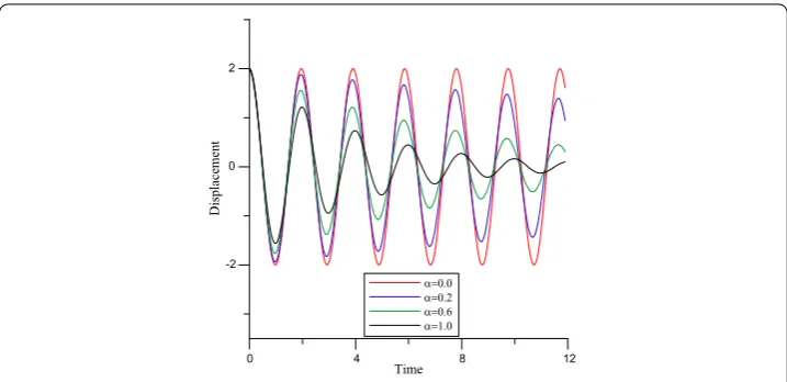
Figure 1 Displacement-time curves for different values of the order of the fractional derivative for

f(x) =xe–x_{(a= 0.8,ε= 0.1,η= 8,λ= 1,x= 0.5).}

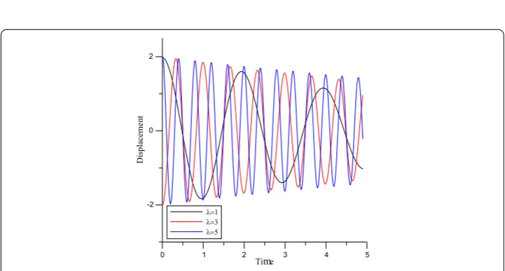
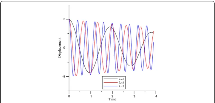
Figure 2 Displacement-time graph for different values ofλforf(x) =xe–x_{(a= 0.5,ε= 0.1,η= 8,}

α= 0.6,x= 0.5).

4.2

ω

ω

ω

ω

If we consider the parametric resonance, then

= ωn+εσn. ()

Hence, the solvability condition requires that

iωnDAn–

a

dA¯ne

iεσnT_+η(iω

n)αAn= , ()

whered is given by (). To perform the stability analysis, one introduces the

transfor-mation

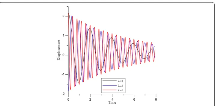
Figure 3 Displacement-time graph for various values ofλforf(x) =x2e–x(a= 0.001,ε= 0.1,η= 8,

α= 0.8,x= 0.5).

whereBncan be written as

Bn(T) =

bR_n+ibI_n eλT_{. ()}

Substituting Eq. () into Eq. () and also obtaining the result placed into Eq. () (and separating into real and imaginary parts), we get

λ+η_ω_nα–sin(π

α) –

d

ωn+ ( η

ω

α–

n cos(πα) –

σn

)

– d

ωn – ( η

ω

α– n cos(

π

α) –

σn

) λ+

η

ω

α– n sin(

π

α)

bR n bI n =   . ()

For a non-trivial solution (bR

n= ,bIn= ), the determinant of the coefficient matrix must be

λ+η ω α– n sin π α  – d

ωn

 – η ω α– n cos π α

–σn 



= . ()

Here,λalso must be zero for the steady-state condition. Thus, the stability boundaries are determined as follows:

σn=ηωαn–cos

π α ± d

ωn



–

ηωα– n sin π α  . ()

Insertingσinto Eq. (), we obtain

= ωn+ε

ηωα_n–cos

π α ± d

ωn



–

ηωα– n sin π α  ()

for the external excitation frequency. Thus, the two different values ofdenote the

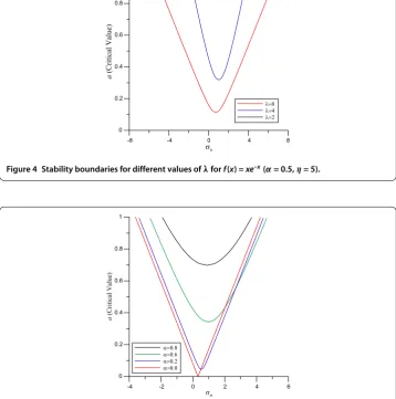
Figure 4 Stability boundaries for different values ofλforf(x) =xe–x(α= 0.5,η= 5).

Figure 5 Stability boundaries for different values ofαforf(x) =xe–x(λ= 5,η= 5).

The variation of an unstable region for different values ofλis observed in Figure . Since the rigidity of the system is increased by decreasing the value ofλ, the unstable region reduces expeditiously for smaller values ofλ.

The variation of an unstable region with some different values ofαforλ=  andη=  is shown in Figure . Here, it is expected that the critical value ofabecomes zero for

α= . This situation is clearly observed in Figure . On the other hand, the unstable region diminishes whileαis increasing. Finally, the effect of the variation ofαon the critical value ofais presented in Figure . Figure  shows that critical valueachanges nonlinearly with the order of fractional derivative.

4.3

ω

ω

ω

ω

This case corresponds to the absence of any resonances. Then, Eq. () turns into

D_w+L[w] =

–iωnDAnXn–η(iωn)αAnXn

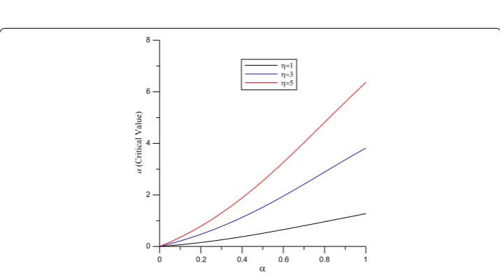
Figure 6 Critical value ofaversus the value ofηfor various fractional orders (λ= 1).

Figure 7 Critical value ofaversus the value ofαfor various damping coefficients (λ= 1).

whereccis a complex conjugate andNSTdenotes non-secular terms. Substituting Eq. () into Eq. (), we obtain the equation

ϕ_n+ω_nϕn= iωnDAnXn+η(iωn)αAnXn ()

with the boundary conditions

ϕn() =ϕn() = . ()

Using the solvability condition [], we find

iωnDAn





X_n(x)dx+η(iωn)αAn





Figure 8 Displacement-time graph for the different fractional order forf(x) =xe–x(ε= 0.1,λ= 1,

η= 5,x= 0.5).

By the normalization, then Eq. () becomes

iωnDAn+ (iωn)αdAn= . ()

Thus, the displacement is obtained as follows:

w(x,t)∼=Aexp

–η

ω

α– n sin

π

α

εt

×

exp

iη

εtω

α– n cos

π

α

+iωnt

+cc

sinωnx

+ cos¯t

sin¯x sin¯

ψ()cos¯–ψ()

–ψ()cos¯x+ψ(x)

. ()

On the other hand, the amplitude is

An(T) =Aexp

i

ω

α– n ηcos

π

α

–η ω

α– n sin

π

α

T

. ()

The displacement-time variation for different values ofα is seen in Figure . Also, it is shown that the damping increases while the value of coefficientλdiminishes in Figure .

4.4

ω

ω

ω

ω

This case deals with the primary resonance=ωn+εσnwhen the frequency of the trans-verse loading is approximately equal to the natural frequency. Then, the steady-state solu-tions of amplitude-phase modulation equasolu-tions and their stability can be discussed. Using the polar form

An=  an(T)e

iβn(T) _()

and substituting Eq. () into the equation below,

Figure 9 Displacement-time graph for different values ofλforf(x) =xe–x_{(ε= 0.1,η= 8,α= 0.5,}

x= 0.5).

where

d=





Xn(x)Y(x)dx, ()

we then obtain

a_n+ianβn–iηωαn–

cos π α

+isin

π

α



an+de i(σnT–βn)

= , ()

whereγn=σnT–βn. Separating the equation into real and imaginary parts and also sub-stituting the equation

a_n=γ_n=  ()

into Eq. (), we find

Re :η ω α– n sin π α

= –d

an

ηωα_n–

cos π α

sinγn+sin

π

α

cosγn

, ()

Im :σn–

η ω α– n cos π α

=d

an

ηωα_n–

cos π α

cosγn–sin

π

α

sinγn

. ()

By the same mathematical manipulation, the stability boundaries are calculated as follows:

σn=

η ω α– n cos π α ±η d ωnα–

a n –  ω α– n sin π α  . ()

4.5 Sum type of resonance (

ω

εσ

In this case, we consider the sum or difference of internal and external forced frequency since= ,= ωn, and=ωn. Likewise, Eq. () is arranged once again; it is found that

iωnDAn+  de

iσnT_+η(iω

d= –a





Xn(x)Y(x)dx. ()

Substituting Eq. () into Eq. () and also separating the equation into real and imaginary parts, we get

Re :a_n+η ω

α– n ansin

π

α

= – d ωn

sinγ, ()

Im :anσn–anγn–

η

ω

α– n ancos

π

α

= d ωn

cosγ. ()

Inserting Eq. () into Eqs. () and (), then we have

Re :η ω α– n sin π α

= – d ωnan

sinγn, ()

Im :σn–

η ω α– n cos π α

= d ωnan

cosγn. ()

Therefore, the stability boundaries are obtained as follows:

σn=

η ω α– n cos π α ±  

d_

ω nan

–η_ωα– n sin

π α . () 5 Conclusion

In this study, the effects of the damping term modeled with a fractional derivative on the dynamic analysis of a beam having viscoelastic properties subject to the harmonic external force are investigated. The parametric or primary resonances in simple supported beams, the governing equation of which involves a fractional derivative, are also analyzed. It is concluded that the value of the natural frequency of the beam modeled with a fractional damper is greater than that of the beam modeled with a classical damper. The fractional derivative has no effect on the static behavior, but it has a significant impact on the dy-namic behavior. Furthermore, it is seen that the unstable region in the resonance case diminishes when the order of the fractional derivative increases.

Competing interests

The authors declare that they have no competing interests.

Authors’ contributions

All authors read and approved the final manuscript.

Author details

1_{Department of Mathematics, Faculty of Art & Science, Celal Bayar University, Manisa, 45047, Turkey.}2_{Department of Civil}

Engineering, Faculty of Engineering, Celal Bayar University, Manisa, 45140, Turkey.

Received: 29 August 2012 Accepted: 19 October 2012 Published: 15 November 2012

References

1. Rossikhin, YA, Shitikova, MV: Application of fractional calculus for dynamic problems of solid mechanics: novel trends and recent results. Appl. Mech. Rev.63, 010801 (2010)

3. Pakdemirli, M, Boyacı, H: The direct-perturbation methods versus the discretization-perturbation method: linear systems. J. Sound Vib.199(5), 825-832 (1997)

4. Galucio, AC, Deu, J-F, Ohayon, R: A fractional derivative viscoelastic model for hybrid active-passive damping treatments in time domain - application to sandwich beams. J. Intell. Mater. Syst. Struct.16, 33-45 (2005)

5. Podlubny, I: Fractional Differential Equations. Mathematics in Science and Engineering, vol. 198. Academic Press, San Diego (1999)

6. Agrawal, OP: Formulation of Euler-Lagrange equations for fractional variational problems. J. Math. Anal. Appl.272, 368-379 (2002)

7. Zhang, Y: A finite difference method for fractional partial differential equation. Appl. Math. Comput.215, 524-529 (2009)

8. Chen, L-Q, Zhao, W-J, Zu, JW: Transient responses of an axially accelerating viscoelastic string constituted by a fractional differentiation law. J. Sound Vib.278, 861-871 (2004)

9. Boyacı, H, Pakdemirli, M: A comparison of different versions of the method of multiple scales for partial differential equations. J. Sound Vib.204(4), 595-607 (1997)

10. Shimizu, N, Zhang, W: Fractional calculus approach to dynamic problems of viscoelastic materials. JSME Int. J. Ser. C Mech. Syst. Mach. Elem. Manuf.42(4), 825-837 (1999)

11. Rossikhin, YA, Shitikova, MV: Application of fractional calculus for analysis of nonlinear damped vibrations of suspension bridges. J. Eng. Mech.124, 1029-1036 (1998)

12. Zhang, L, Zu, JW: Nonlinear vibration of parametrically excited moving belts, part I: dynamic response. J. Appl. Mech. 66(2), 396-403 (1999)

13. Öz, HR, Pakdemirli, M, Boyacı, H: Non-linear vibrations and stability of an axially moving beam with time dependent velocity. Int. J. Non-Linear Mech.36, 107-115 (2001)

14. Pakdemirli, M, Boyacı, H: Comparison of direct-perturbation methods with discretization-perturbation methods for nonlinear vibrations. J. Sound Vib.186, 837-845 (1995)

15. Nayfeh, AH: Introduction to Perturbation Techniques. Wiley-Interscience, New York (1981)

doi:10.1186/1687-2770-2012-135