R E S E A R C H
Open Access
A note on the shooting method and its
applications in the Stieltjes integral boundary
value problems
Huilan Wang, Zigen Ouyang
*and Hengsheng Tang
*Correspondence: [email protected]
School of Mathematics and Physics, University of South China, Hengyang, 421001, P.R. China
Abstract
In this paper, the existence results of positive solutions for three-point
Riemann-Stieltjes integral BVPs (boundary value problems) is considered. By applying shooting method and comparison principle, we obtain some new results which extend the known ones. At the same time, the theorems in one of our published articles are corrected by another theorem in this paper.
MSC: 34B10; 34B18; 34C10
Keywords: integral boundary value problem; existence; positive solution; shooting method; comparison principle
1 Introduction
By applying the shooting method, we establish the criteria for the existence of positive solutions to the following Riemann-Stieltjes integral BVPs:
u(t) +a(t)fu(t)= , <t< , (.)
u() = , u() =α
η
u(s)ds, (.)
wheref ∈C([,∞); [,∞)) and <η< ,α≥ are given constants, and <αη< . Set
f= lim u→+
f(u)
u , f∞=ulim→∞
f(u)
u ,
¯
fx=lim u→xsup
f(u)
u , fx=ulim→xinf
f(u)
u , x∈ {, +∞}.
By Krasnoselskii’s fixed point theorem in a cone, Tariboon and Sitthiwirattham [] proved that BVP (.)-(.) has a positive solution in the casef= andf∞=∞(super-linear case) or in the casef=∞andf∞= (sub-linear case) when <αη< .
Some meaningful results of nonlinear second-order integral BVPs have already been obtained by Kong [], Webb and Infante [, ],etc.The following BVP:
u(t) +fu(t)= , <t< ; u() = , u() =α
η
u(s)ds, (.)
is a special case of Webb and Infante’s [], where we can deduce the result. Suppose <αη< ; BVP (.) has at least one positive solution if one of the following conditions holds:
(i) f¯<μandf∞>μ;
(ii) f¯>μandf∞<μ,
whereμ= /r(L) andr(L) is the spectral radius of the associated linear operator. In [], the authors used fixed point index theory.
As a numerical method, the shooting method is efficient to find the solution of BVPs [–]. Kwong and Wong [] obtained some results for the Robin boundary condition of the form
sinθu() –cosθu() = , u() – m–
i=
αiui(ηi) = , (.)
whereθ∈[, π/] andθ=π/. Kwong and Wong [] showed that BVP (.) with (.) has at least one positive solution iff¯<Lθandf∞>Lθ, whereLθis a certain but not specified
constant related to the associated linear operator.
Whenθ =π/ and ≤mi=–αiηi< , Ma [] has studied BVP (.) with (.) by using Krasnoselskii’s fixed point theorem in a cone. The sufficient condition for the existence of positive solutions is also the super-linear case or the sub-linear case.
Whena(t)≡,m= ,η= /, as a special case of [], the BVP
u(t) +fu(t)= , <t< ; u() = , u() =μu(η), (.) was studied by Kwong in [], where the existence condition is
¯
f<
cos–
μ
<f∞, or f¯∞<
cos–
μ
<f
, (.)
which is obtained by the shooting method.
Following the main idea in [, ], we considered the generalized multi-point integral BCs []
u() = , u() = n
i= αi
ηi
u(s)ds, (.)
where <η<η<· · ·<ηn< ,αi≥ fori= , . . . ,n– , andαn> are given constants. However, Theorem . and some proofs in [] need to be corrected, which is one of the reasons why we write this paper. Furthermore, more general existence criteria are pre-sented in this article as well as the application of the shooting method in the study of BVPs. For simplicity and without loss of generality, we start from BVP (.)-(.).
2 Preliminaries: some notation and lemmas
The principle of the shooting method is converting the BVP into an IVP (initial value problem) by finding suitable initial slopesm> such that the solution of (.) comes with the initial value condition
Denote byu(t,m) the solution of the IVP (.) with (.) provided it exists, and define
k(m) =α
η
u(s,m)ds
u(,m) , ϕ(m) =α
η
u(s,m)ds–u(,m). (.)
Then solving the boundary value problem is equivalent to finding am∗such thatk(m∗) = orϕ(m∗) = .
For the sake of convenience, we denote
max
≤t≤
a(t)=aL, min
≤t≤
a(t)=al.
In this paper, we always assume
(H) f ∈C([,∞); [,∞)),a∈C([, ]; [,∞)).
Furthermore, we assume thatf is strong continuous enough to guarantee thatu(t,m) is uniquely defined and that it depends continuously on both t and m. As for the discussion of this problem, see [].
Next, we present some comparison theorems which help us to establish the main results.
Lemma .(Sturm comparison theorem) Letϕ andϕ be non-trivial solutions of the
equations
y+q(x)y= , y+q(x)y= ,
respectively,on an interval I;here qand qare continuous functions such that q(x)≤q(x)
on I.Then between any two consecutive zeros xand xofϕ,there exists at least one zero
ofϕunless q(x)≡q(x)on(x,x).
Lemma . Let y(t,m),z(t,m),Z(t,m)be the positive solution of the initial value problems,
respectively,
y(t) +fy(t)= , y() = , y() =m,
Z(t) +G(t)Z(t) = , Z() = , Z() =m,
z(t) +g(t)z(t) = , z() = , z() =m.
Suppose g(t)≤G(t)be two piecewise continuous functions defined on[, ].If
≤g(t)≤f(y(t))
y(t) ≤G(t)
and suppose that Z(t)does not vanish in(, ],then for any≤s≤ξ≤,it yields
z(s,m)
z(ξ,m)≤
y(s,m)
y(ξ,m)≤
Z(s,m)
Z(ξ,m), (.)
and hence,for any≤η≤ξ≤,we have
η
z(s,m)ds
z(ξ,m) ≤
η
y(s,m)ds
y(ξ,m) ≤
η
Z(s,m)ds
Proof Since ≤ g(t) ≤ f(y(t))/y(t)≤ G(t) and Z(t) does not vanish in (, ], from Lemma ., it follows thaty(t) andz(t) will not vanish in (, ]. The proof for (.) can be seen in []. The continuity of the integrands implies the existence of the Riemann in-tegral. In view of the definition of Riemann integral, by using the inequality of the limit,
we have (.).
Remark . Lemma . is also the correction for Theorem . in [].
Lemma . Consider the BVP
y(t) +Ay(t) = , <t< , (.)
y() = , y() =b. (.)
(i) IfA=π,theny(t)vanishes att= for the first time on interval(, ]andb= ; (ii) if <A<π,theny(t)does not vanish on the interval(, ]andb> ;
(iii) ifA>π,theny(t)vanishes beforet= on interval(, ].
Proof Obviously,y(t) =sin(πt) satisfies the conditionsy() = ,y() = , andy(t) > for
t∈(, ), hence (i) is established. According to the Sturm comparison theorem, we can
draw the conclusions (ii) and (iii).
Lemma .([]) Assume that(H)holds andαη> ,then BVP(.)-(.)has no positive
solution.
In [] and [], the proofs are conducted by contradiction to the concavity of solution (also see []). In fact, form> , we compare the solutionu(t,m) of the IVP given by (.) and (.) with the solutiony(t) =mtof
y(t) + y(t) = , y() = , y() =m. (.)
If BVP (.)-(.) has a positive solutionu(t,m), then by Lemma . and the concavity of
u(t,m), we have
η≥
u(,m)
u(η,m)=
α ηu(s,m)ds
u(η,m) ≥
α ηy(s,m)ds
y(η,m) =
α ηms ds
mη =
αη
, (.)
that is,αη≤.
In the following, we always assume that
(H) <αη< .
3 Main results
Lemma . Assume that(H)-(H)holds.Then there exist a solution x=A∈(,π)such
that
g(x) :=α[ –cos(ηx)]
and a solution x=A∈(,π)such that
g(x) :=αηsin(ηx)
sinx = . (.)
Proof It is not difficult to show that
lim
x→+g(x) =
αη
< , xlim→π–g(x) =∞> .
Since the functiong(x) is continuous on (,π), there must exist a constantA∈(,π) such thatg(A) = .
Similarly,
lim
x→+g(x) =
αη
< , xlim→π–g(x) =∞> .
Thus, there exists a positive constantA∈(,π) such thatg(A) = .
Theorem . Assume that(H)-(H)holds.Suppose one of the following conditions holds:
(i) ≤ ¯f<
A
aL, f∞> ¯
A
al; (ii) ≤ ¯f∞<
A
aL, f> ¯
A
al.
Then problem(.)-(.)has at least one positive solution,where
A=min{A,A}, A¯=max{A,A},
and A,Ais defined in(.)and(.),respectively.
Proof (i) Since ≤ ¯f<A
aL, there exists a positive numberrsuch that
f(u)
u < A aL ≤
A
aL , <u≤r. (.)
Let <m∗<r, then from the Sturm comparison theorem and the concavity ofu(t,m∗), it follows that ≤u(t,m∗)≤m∗t≤m∗<rfort∈[, ]. Thus
≤a(t)fut,m∗<aLA
aLu
t,m∗=Aut,m∗<πut,m∗, t∈(, ]. By Lemma ., it givesu(t,m∗) > fort∈(, ].
LetZ(t) = (m∗/A)sin(At) fort∈[, ], then
Z(t) +AZ(t) = , Z() = , Z() =m∗. (.)
From Lemma . and Lemma ., we have
km∗=α
η
u(s,m∗)ds
u(,m∗) <
α ηm∗sin(As)ds
m∗sinA
=α[ –cos(ηA)]
AsinA
= , (.)
On the other hand, the second inequality in (i) implies that there exists a numberLlarge enough such that
f(u)
u >
¯
A
al ≥
A
al, u≥L, (.)
and there exists a positive number<A( –η)/ηsmall enough that
f(u)
u ≥
(A+)
al , u≥L. (.)
Next, we will find a positive numberm∗such thatϕ(m∗)≥.
Claim. There exist a slopem∗and two positive numbersρandσsuch that
<ρ≤η≤ A
A+ ≤
σ≤ and ut,m∗≥L fort∈[ρ,σ].
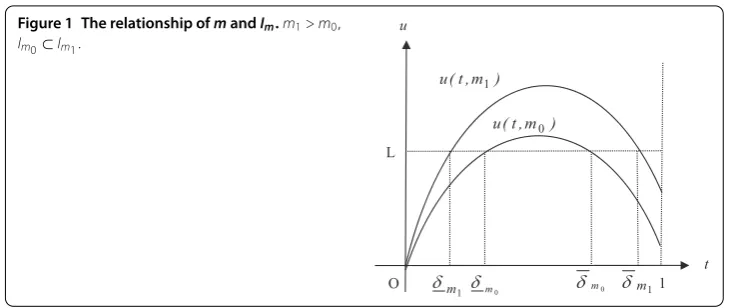
Since the solution u(t,m) is concave, it hits the lineu=Lat most two times for the constant L defined in (.) and t∈(, ]. We denote the left intersecting time by δm and the right one by δm provided they exist. Henceforth, denoteIm= [δm,δm]⊆(, ]. Ifu(,m)≥L, thenδm= .
The discussion is divided into three steps.
Step. We claim that there exists a slopemlarge enough such that ≤u(t,m)≤Lfor
t∈[,δm] andu(t,m)≥Lfort∈Im.
Otherwise, providedu(t,m)≤Lfor allt∈[, ] asm→ ∞, then by integrating both sides of (.) from tot, we have
u(t,m) =mt–
t
(t–s)a(s)fu(s,m)ds. (.)
Hence, from (.) and the continuity off(u), we have
m=u(,m) +
( –s)a(s)fu(s,m)ds≤L+LfaL, (.)
whereLf =maxu∈[,L]f(u). If we choosem>L+LfaL, (.) will lead to a contradiction. Sinceu(t,m) is continuous and concave, there exists a numbermlarge enough such thatu(t,m)≥Lfort∈Im.
Step. There exists a monotonically increasing sequence{mk}such that the sequence δm
kis decreasing onmkandδmkis increasing onmk. That is,
Im⊂Im⊂ · · · ⊂Imk⊂ · · · ⊆(, ]
andu(t,mk)≥Lfort∈Imk. First, we prove that
δm
k<δmk–, k= , . . . formk>mk–. (.)
Whenk= , we have
u(δm
Figure 1 The relationship ofmandIm.m1>m0,
Im0⊂Im1.
in the case
m>m+ aLLfδm. (.)
Otherwise, provided
u(δm
,m)≤u(δm,m) =L, (.)
then from (.) and (.), we have
u(δm
,m) –u(δm,m)
= (m–m)δm–
δm
(δm–s)a(s)fu(s,m)
–fu(s,m)
ds
> (m–m)δm– a
LL fδm
=δm(m–m) – aLLfδm
> ,
which contradicts (.).
Hence, for a slopem>m+ aLLfδm, there exists a number <δm<δmsuch that
u(δm,m) =L, and u(t,m)≤L fort∈(,δm].
See Figure .
By mathematical induction, it is not difficult to show thatδm
k <δmk–,k= , , . . . .
Further, we turn to the right hand of the intervalImk. Sincef guarantees thatu(t,m) is uniquely defined, the solutionsu(t,mk–) andu(t,mk) have no intersection in the interval [δmk–, ). It follows from
u(δm
k–,mk) >u(δmk–,mk–)
that
Figure 2 Two of the possible cases ofIm0.Subcase 1:η∈[δm0,δm0] andu(1,m0)≥L; Subcase 2:
η[δm0,δm0] oru(1,m0) <L.
Thus we have
δmk>δmk–, k= , , . . . formk>mk–. (.)
Whenk= , also see Figure .
Step. Seek out a slopem∗and two positive numbersρ andσ such that <ρ≤η≤ A
A+ ≤σ≤ andu(t,m
∗
)≥Lfort∈[ρ,σ].
Subcase.η∈[δm
,δm] andu(,m)≥L. In this case, we takem∗=mandρ=δm,
σ=δm= .
Subcase.η[δm
,δm] oru(,m) <L. Following the step , step , and the extension
principle of solutions, there exists a positive integernlarge enough such that
δmn<η, δmn≥
A
A+
. (.)
If we takem∗=mnandρ=δmn,σ=δmn, then
σ(A+)≥A. (.)
Two of the possible cases ofImcan be seen in Figure .
In the following, we prove thatk(m∗)≥ orϕ(m∗) > for the selectedm∗andρ,σ. Setz(t) = (m∗/σ(A+))sin(σ(A+)t), then
z(t) +σ(A+)z(t) = , z() = , z() =m∗, t∈[ρ,σ], (.)
whereρ≤η<σ≤. From (.), we have
f(u)
u ≥
σ(A +)
al , u≥L.
Further, noting thatu(,m∗) >L(this timeσ= ) oru(,m∗)≤u(σ,m∗) =Land the func-tion
S(x) =sinηx
is increasing forx∈(,π), then by Lemma ., Lemma ., and inequality (.), we have
km∗=α
η
u(s,m∗)ds
u(,m∗) ≥
αηu(η,m∗) u(,m∗) ≥
αηu(η,m∗) u(σ,m∗)
≥αηsinησ(A+) sinσ(A+)
≥αηsin(ηA) sinA
= , (.)
which impliesϕ(m∗)≥.
From (.) and (.), we can find am∗ betweenm∗ andm∗ such thatu(t,m∗) is the solution of (.)-(.). The theorem is complete.
The proof for (ii) is similar, so we omit it.
Now, we present the result for BVP (.) with (.), which is also the correction of The-orem . and TheThe-orem . in [].
Theorem . Assume that(H)-(H)hold.Suppose one of the following conditions holds:
(i) ≤ ¯f<
A
aL, f∞> ¯
A
al; (ii) ≤ ¯f∞<
A
aL, f> ¯
A al.
Then problem(.)with(.)has at least one positive solution,where
A=min{A,A}, A¯=max{A,A}
and A,Ais defined by
n
i=αi[ –cos(Aηi)]
AsinA
= (.)
and
n
i=αiηisin(Aηi) sinA
= . (.)
Proof Similar to (.) and (.), it follows from (.) and (.)-(.) that
km∗=
n i=αi
ηi
u(s,m∗)ds
u(,m∗) <
n i=αi
ηi
m∗sin(As)ds
m∗sinA
=
n
i=αi[ –cos(Aηi)]
AsinA
= (.)
and
km∗=
n i=αi
ηi
u(s,m∗)ds
u(,m∗) ≥
n
i=αiηiu(ηi,m∗) u(,m∗) ≥
n
i=αiηiu(ηi,m∗) u(σ,m∗)
≥
n
i=αiηisin(ηiσ(A+)) sinσ(A+) ≥
n
i=αiηisin(Aηi) sinA
= , (.)
whereηn<σ≤ and (.) holds.
4 Conclusion and discussion
The conditions in [] and [] are easy to verify; however, they are not as general as ours, because the sup-linear case or the sub-linear case is sufficient for the conditions in Theo-rem .. As an example of [], where the constantμis related to the Green’s function and the spectral radius of associated linear operator, our calculation is more direct. The idea of this paper was illuminated by [, ]; however, the certain constantLθcould not be given
explicitly in [] andηonly equals / in []. From this point of view, this paper extends the work of [, ] and presents another way to find the ‘eigenvalue’ by numerical calculation, though it is related to a transcendental equation which has at least one numerical solution.
In fact, we can extent our results to []. The proof is fit, where
k(m) =
m–
i= αiu(ηi,m)
u(,m)
and the constantA=A=A∈(,π) is explicitly determined by
m–
i= αisin(Aηi)
sinA = . (.)
In other words, we can substitute the condition
(i) f= andf∞=∞, or
(ii) f=∞andf∞= ,
with
(i) ≤ ¯f<A<f∞; or
(ii) ≤ ¯f∞<A<f,
whereAis defined in (.).
Next, we apply the result to the special case BVP (.), whereaL=al= ,m= ,α=μ, η= /. From (.), we have
A= cos–
μ
.
By plugging it into (i) and (ii), we have the same result as (.).
Further, whenαη= , BVP (.)-(.) is at resonant. There may not exist a solution
x=A ∈(,π) andx=A ∈(,π) to (.) and (.), respectively. If (.) and (.) has a solution x=A ∈(,π) and x=A∈(,π), respectively, then we can also obtain the existence result for (.)-(.), similarly for (.) with (.).
Whenθ=π/ andmi=–αiηi= , BVP (.) with (.) is resonant. If there exists a num-ber A∈(,π) such that (.), then the existence result for BVP (.) with (.) can be obtained, similarly for BVP (.).
Competing interests
The authors declare that they have no competing interests.
Authors’ contributions
Acknowledgements
It was remarked to the authors by Professor Webb that the result is not correct in [9]. The authors would like to express their sincere gratitude to Professor Webb for his helpful comments and suggestion on the manuscript, as well as the anonymous reviewers’ comments. Moreover, the first author HW is sorry for having cited the comparison theorem by mistake in [9]. This project was supported by the Scientific Research Fund of Hunan Provincial Educational Department (No. 13A088), the Scientific Research Foundation of Hengyang City (No. 2012KJ2) and the Construct Program in USC.
Received: 15 October 2014 Accepted: 25 May 2015
References
1. Tariboon, J, Sitthiwirattham, T: Positive solutions of a nonlinear three-point integral boundary value problem. Bound. Value Probl.2010, Article ID 519210 (2010)
2. Kong, LJ: Second order singular boundary value problems with integral boundary conditions. Nonlinear Anal.72(5), 2628-2638 (2010)
3. Webb, JRL, Infante, G: Non-local boundary value problems of arbitrary order. J. Lond. Math. Soc.79(2), 238-258 (2009) 4. Webb, JRL, Infante, G: Positive solutions of nonlocal boundary value problems: a unified approach. J. Lond. Math. Soc.
74(2), 673-693 (2006)
5. Agarwal, RP: The numerical solution of multipoint boundary value problems. J. Comput. Appl. Math.5, 17-24 (1979) 6. Kwong, MK: The shooting method and multiple solutions of two/multi-point BVPS of second-order ODE. Electron.
J. Qual. Theory Differ. Equ.2006, 6 (2006)
7. Kwong, MK, Wong, JSW: The shooting method and nonhomogeneous multipoint BVPs of second-order ODE. Bound. Value Probl.2007, Article ID 64012 (2007)
8. Ma, RY: Positive solutions of a nonlinearm-point boundary value problem. Comput. Math. Appl.42, 755-765 (2001) 9. Wang, HL, Ouyang, ZG, Wang, LG: Application of the shooting method to second-order multi-point integral
![Figure 2 Two of the possible cases of Im0. Subcase 1: η ∈ [δm0,δm0] and u(1,m0) ≥ L; Subcase 2:η ⊈ [δm0,δm0] or u(1,m0) < L.](https://thumb-us.123doks.com/thumbv2/123dok_us/497908.2048896/8.595.118.479.81.232/figure-possible-cases-im-subcase-dm-dm-subcase.webp)