Department of Mathematics
PhD in Mathematics
XXX CYCLE
Model Order Reduction and its Application to an
Inverse Electroencephalography Problem
PhD Student:
Advisors:
Juan Luis Valerdi Cabrera
Alberto Valli
Ana Alonso Rodriguez
Prof. Gianlugi Rozza Scuola Internazionale Superiore di Studi Avanzati - SISSA
Quisiera expresar mi gratitud a las personas que me han seguido en la trayectoria del doctorado. Agradezco a los profes Alberto Valli y Ana Alonso por el apoyo brindado en cada encuentro y por darme la oportunidad de hacer el doctorado con ellos. Gracias a mis colegas de doctorado por compartir momentos de risa y apoyo en nuestra larga jornada: Giulia Tini, Chiara Benazzoli, Marco Oppio, Elena Gaburro, Roberto Civino, Alberto Melati, Riccardo Longo, Daniel Wessel y Christian Contarino.
Quisiera dar una mención especial a Marco Oppio por estar a mi lado en los momentos más difíciles del doctorado y ayudarme a aclarar mi mente en muchas ocasiones. Por supuesto, no olvidaré cuanto me has hecho reír! Gracias amigo.
También quisiera dar unos agradecimientos especiales a mis tres compañeras de oficina, Giulia, Chiara e Elena por los buenos tiempos y las conversaciones que compartimos juntos.
Doy las gracias a mis amigos Sara Dari, Marion Llagiu, Bruno Llagiu, Valentina Tonon, Alejandra Huitrado y Giorgia Tosoni por la especial convivencia que tuvimos en la residencia y los buenos momentos que compartimos juntos.
El ultimo año fue posiblemente el más difícil pero a la vez uno de los más lindos gracias a la llegada de dos cosas: el squash y el amor. Gracias a mis compañeros de squash Ramu Peretti y Matteo Magagnini por la intensidad y el entusiasmo en el campo de juego.
El amor llego con el nombre de Elena Remonato. Gracias por cada sonrisa y abrazo que lleno mi vida de colores. También quisiera agradecer tu paciencia y apoyo, y sobretodo la fuerza que me brindaste para poder terminar. Gracias también a tu familia por acogerme como un miembro más, cuantos momentos en lindos!
Por ultimo quiero agradecer a las personas mas importantes de mi vida, mi familia, que aunque estuvieron lejos me apoyaron en todo momento de esta travesía: Mima, Abuelata, tia Aleida, tia Nidia, Aimara, Indira, Tomasito y Evelyn.
A mis padres les quiero dedicar un agradecimiento especial. Llegar a la culminación de este sueño es fruto de su amor sin límites. Todo lo que he obtenido en mi vida es gracias al sostén incondicional que me han dado. Hoy nos graduamos los tres.
El doctorado ha sido el momento de crecimiento personal más grande que he tenido y es en gran parte gracias a los momentos especiales que compartí con todas estas personas. Gracias de corazón.
Vorrei esprimere la mia gratitudine alle persone che mi hanno seguito nel percorso del dottorato. Ringrazio i professori Alberto Valli e Ana Alonso per avermi dato l’opportunità di lavorare con loro e per il supporto fornitomi in ogni incontro. Grazie ai miei colleghi di studio per aver condiviso momenti di risate e per tutto il sostegno datomi in questo lungo viaggio: Giulia Tini, Chiara Benazzoli, Marco Oppio, Elena Gaburro, Roberto Civino, Alberto Melati, Riccardo Longo, Daniel Wessel e Christian Contarino.
Vorrei fare un ringraziamento speciale a Marco Oppio per essere stato al mio fianco nei momenti più difficili del dottorato ed avermi aiutato a chiarire la mente in molte occasioni. Certo, non dimenticherò quanto mi hai fatto ridere! Grazie amico.
Vorrei anche ringraziare in modo speciale i miei tre colleghi di ufficio, Giulia, Chiara ed Elena per i bei momenti e le conversazioni che abbiamo condiviso insieme.
Ringrazio i miei amici Sara Dari, Marion Llagiu, Bruno Llagiu, Valentina Tonon, Alejandra Huitrado e Giorgia Tosoni per la bella convivenza allo studentato e i bei momenti che abbiamo trascorso assieme.
L’ultimo anno è stato forse il più difficile, ma allo stesso tempo uno dei più belli grazie all’arrivo di due cose: lo squash e l’amore. Grazie ai miei colleghi di squash Ramu Peretti e Matteo Magagnini per l’intensità e l’entusiasmo in campo.
L’amore è arrivato col nome di Elena Remonato. Grazie per ogni sorriso ed abbraccio che hanno riempito la mia vita di colori. Vorrei anche ringraziare la tua pazienza e il tuo supporto e soprattutto la forza che mi hai dato per poter finire. Grazie anche alla tua famiglia per avermi accolto come un membro in più, quanti momenti belli!
Infine vorrei ringraziare le persone più importanti della mia vita, la mia famiglia. Chi, nonostante la lontananza, mi ha sostenuto in ogni momento di questo viaggio: Mima, Abuelata, zia Aleida, zia Nidia, Aimara, Indira, Tomasito ed Evelyn.
Ai miei genitori vorrei dedicare un ringraziamento speciale. Raggiungere il culmine di questo sogno è il frutto del vostro amore senza limite. Tutto ciò che ho ottenuto nella mia vita è stato possibile grazie al supporto incondizionato che mi avete dato. Oggi ci dottoriamo tutti i tre.
Il dottorato è stato il più grande momento di crescita personale che abbia avuto ed è in gran parte dovuto ai momenti speciali che ho condiviso con tutte queste persone. Grazie dal cuore.
Introduction 1
1 Elements of RB and FOR Methods 7
1.1 Abstract Framework . . . 7
1.2 Reduced Basis Offline Stage . . . 10
1.3 Reduced Basis Online Stage . . . 16
1.4 Kolmogorov’s n-width Estimates . . . 19
1.5 Fundamental Order Reduction Method . . . 27
1.6 Reduced Basis Error Estimates . . . 38
1.7 Empirical Interpolation Method . . . 45
2 RB and FOR on an Epilepsy EEG Equation 50 2.1 Subtraction Approach Formulation. . . . 51
2.1.1 RB on the Subtraction Approach. A Simple Case . . . 52
2.1.2 RB and FOR on the Subtraction Approach. A More Realistic Case . . . 64
2.2 Direct Approach Formulation . . . . 71
2.2.1 RB on the Direct Approach . . . 72
2.3 Solution for the EEG Inverse Problem . . . 76
3 jMOR 89 3.1 POD on the Laplacian operator . . . 90
3.2 jMOR Functions Reference . . . 98
Conclusions 101
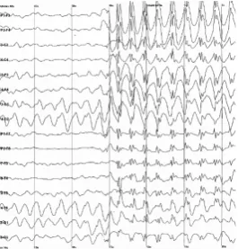
1 Epileptic spike detected with EEG . . . 4
1.1 Reduced basis set relations . . . 11
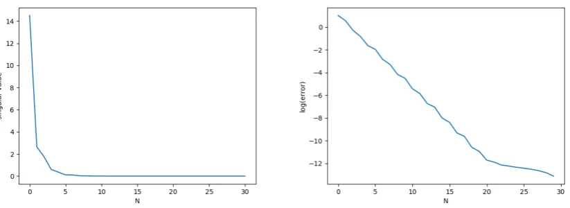
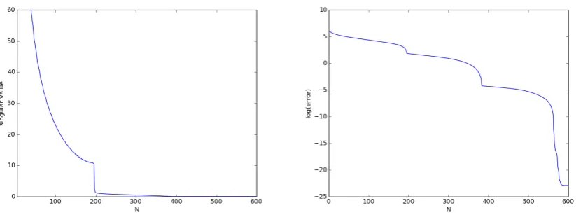
2.1 DomainΩdivided by layers. . . 56 2.2 RB in a compact set, isotropic subtraction approach case. Singular values and error
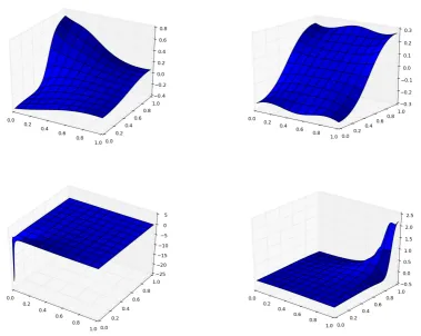
estimates . . . 57 2.3 RB in a compact set, isotropic subtraction approach case. Some test errors ink · kH1(Ω) 57
2.4 RB for P ≈ Ω, isotropic subtraction approach case. Singular values and error estimates . . . 62 2.5 RB forP≈Ω, isotropic subtraction approach case. Some test errors ink · kH1(Ω) . 62
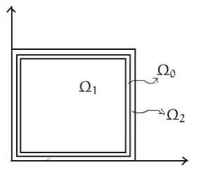
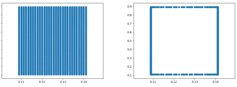
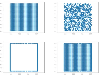
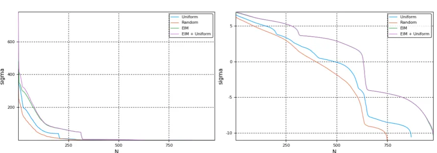
2.6 Isotropic subtraction approach case. Truth solutions for different sources . . . 63 2.7 Subdomains ofΩ:Ω0, Ω1, Ω2. . . 64 2.8 EIM in a compact set, anisotropic subtraction approach case. EIM sampling onu0 . 66 2.9 RB in a compact set, anisotropic subtraction approach case. Sampling schemes . . 67 2.10 RB in a compact set, anisotropic subtraction approach case. Singular values and
error estimates . . . 68 2.11 RB in a compact set, anisotropic subtraction approach case. Exact error for different
parameters . . . 68 2.12 MOR in a compact set, anisotropic subtraction approach case. Exact error difference
between RB and FOR . . . 70 2.13 MOR in a compact set, anisotropic subtraction approach case. Comparison between
RB and FOR . . . 70 2.14 RB in a compact set, isotropic direct approach case. Singular values . . . 73 2.15 RB in a compact set, isotropic direct approach case. Projection error estimates inΞs 73 2.16 RB in a compact set, isotropic direct approach case.l2error withµ∈Ξs . . . 74 2.17 RB in a compact set, isotropic direct approach case.l2error withµ6∈Ξs . . . 74 2.18 Isotropic direct approach case. Two truth solutions . . . 75 2.19 RB in a compact set, isotropic direct approach case. Reduced basis functions . . . . 75 2.20 Simulated annealing on the EEG inverse problem. Average computing times . . . . 79 2.21 Approximation of the inverse EEG function. Average error in the training setΞtr
2.22 Approximation of the inverse EEG function,q=16. Comparison between actual and estimated parameter, Example 1. . . 86 2.23 Approximation of the inverse EEG function,q=16. Comparison between actual
and estimated parameter, Example 2. . . 86 2.24 Approximation of the inverse EEG function. Average error in the training setΞtr
and the test setΞte . . . 87 2.25 Approximation of the inverse EEG function,q=128. Comparison between actual
and estimated parameter, Example 1. . . 87 2.26 Approximation of the inverse EEG function,q=128. Comparison between actual
and estimated parameter, Example 2. . . 88
A scientific or engineer simulation is a way to reproduce a phenomenon of the real world in order to predict an output given some input of the modeled system. These simulations have great impact in everyday life as well as in engineering and science itself, e.g. weather forecast [133], civil engineering [78], biology [119], etc. A huge body of simulations are modeled by partial differential equations (PDE), which represent a wide variety of phenomena such as sound, heat, electrostatics, electrodynamics, fluid flow, elasticity, etc. [28, 67, 77, 139].
Nowadays there are diverse successful methods for numerically solving PDEs like finite element methods (FEM) [52, 132], finite volume methods (FVM) [120], spectral methods [44, 45], among others. Sometimes computing ahigh-fidelityorfull-orderapproximation of a very complex PDE through these methods can be very demanding and the computation in supercom-puters could take from hours to days to finish. Furthermore, in the case of PDEs depending on parameters, i.e.parameterized PDE, the computation of solutions for many different parameters may be extremely expensive or even impossible due to time constraint, like for example, in
inverse problems or optimal controlwhere an iterative procedure needs to solve the forward problem several times [90]. This setting where a PDE has to be solved numerous times with
different configuration of parameters is commonly known as amany-query context.
A simple example of a parametrized PDE is shown by the following equation: Given
µ∈P⊂Rp, solve
−div(σ(µ)∇u) = f(µ) inΩ, u = 0 onΓD, σ(µ)∇u·n = 0 onΓN.
where the parameter setPrepresents a compact subset ofRp, p≥1; the domainΩ⊂Rd, d≥1, denotes an open bounded and connected region with Lipschitz boundary,∂Ω = ΓD∪ΓN the boundary ofΩandnthe outward unit normal vector on∂Ω. Hereσandfare two parameter-dependent functions
σ, f:P×Rd→R.
In general, the parameters may lay in any position of the model, i.e. in the domain, bound-ary or initial conditions, source terms, or in the physical properties.
MOR is not a new idea, it has been used since the 70s in many-query design evaluation [70] and parameter continuation methods [6]. Afterwards, they were further developed to other problems like differential equations throughreduced basis(RB) methods [24, 69, 105]. Nevertheless, they did not have strong emphasis in thecertificationof the error which is very important because MOR techniques may be susceptible to inaccuracies on the solution. To bring rigor to these methods, a-posteriori error estimates and effective sampling strategies were researched and published at the beginning of the 00s [57, 130, 135, 165]. Nowadays, reduced basis methods are widely applied and very actively researched in numerous fields, e.g. Maxwell equations [49, 50, 51], Stokes equations [71, 134, 138], homogenization [37, 121], multi-scale methods [1, 2, 98], parabolic equations [74, 76], nonlinear problems [46, 75, 95], optimal control [59, 136, 155, 156], uncertainty quantification [38, 87, 122] and many others. There are two main algorithms to apply RB to PDEs: proper orthogonal decomposition (POD) andgreedy.
The idea of POD is to represent a collection of solutions of the differential equation with an orthonormal basis which is optimal in a least-square sense. This representation is built from a small dimensional space and retains the most important information of the solutions. One of its first application appeared in turbulent flows [11, 12, 147, 148] and nowadays is used in many other kind of equations [13, 42, 96, 97, 102, 103, 155].
As an alternative to POD we could use greedy algorithms. Differently from POD, a greedy approach does not need a precomputed collection of solutions, which can save computational time in many cases. It uses a-posteriori error estimates to select the most meaningful parameters to construct the reduced model while minimizing the computation of full-order solutions. The first greedy method was introduced in the 70s [64] and was related to optimization problems. Later by the 00s greedy methods were studied in the RB context [113, 114, 137, 142, 165], mainly for a-posteriori error estimation and a-priori convergence.
In general, RB methods use anoffline-onlineapproach which means there are two stages: • offline stage: take advantage of the parametric dependence of the PDE and, for a selection of parametersµj∈Pcompute the corresponding high-order solutions, also called in this contextsnapshots, that will constitute the reduced basis. This stage is done only once. • online stage: use the small dimension of the RB to compute a fast approximation of the
high-order solution for a given parameter inµ∈P,µ6=µj.
The computations in the offline stage are carried out by usual numerical techniques, e.g FEM. This stage can take a huge amount of time to finish but once done the results are used and stored to build a reduced model. Then, the offline-online decoupling replaces the large algebraic system of the legacy methods by a smaller one, whose dimension is controlled by the dimension of the RB. This approach gives remarkable speedups to the point ofreal time evaluation of PDEs [10, 57, 122, 130, 134, 164].
A case in which we can obtain real time computations in the online stage is when we have an affine representation of the parametric part of the PDE, i.e.
f(x;µ) =
Qf
X
q=1
This helps having less computational burden in the online stage because many operations can be precomputed in the offline stage. For example, given an linear operatorAwe obtain
Af(x;µ) =
Qf
X
q=1
Θqf(µ)Afq(x),
and after we have computedAfq(x)for allq=1, . . . , Qf, evaluatingAffor different parameters is inexpensive.
In the case there is not an affine representation of the parametric part we can return to that case by using theempirical interpolation method(EIM). It was introduced in [23] and since then is the standard method for computing affine representations. This method is iterative and hierarchical, it achieves exponential convergence rate for analytical functions and is applicable in general domains.
The fast computation in the state of the art of RB methods is outstanding. Nevertheless, one of the aim of this thesis is to take it further.
Objective 1:Improve computational times in the online stage of reduced basis methods while
retaining good accuracy.
To achieve this objective we propose two ideas: theFundamental Order Reduction Method (FOR) andoffline error estimators.
In Section 1.5 we propose the fundamental order reduction method for solving PDEs dependent of parameters. Differently from POD and greedy, the FOR method uses nonlinear combinations of the snapshots to build the new basis and does not solve the PDE from the reduced model in the online stage. In the online stage the only operations executed are simple affine evaluations like in (1).
The FOR method is not completely new, it appears in [131], but not as solver of parametric PDEs, instead as an estimator on the accuracy we could obtain from a reduced basis in finite dimensional spaces. We expand all the results found in [131] to infinite dimensional spaces and introduce new a-priori convergence results.
We also discuss in Section 1.5 some disadvantages, for example, FOR cannot be applied to all kinds of PDEs so it is not as general as POD and greedy. Also, some of the error estimates can be difficult to obtain in infinite dimensional spaces, whereas in finite dimensional spaces they are easy to compute.
For cases where FOR cannot be used, we propose in Section 1.6 some offline error estima-tors for standard RB techniques. After computing a RB solution the most common procedure is to estimate an a-posteriori error to certify good accuracy. Offline estimators are a class of estimators that move a-posteriori operations to the offline stage, reducing in this way the load of computations in the online stage.
In Section 1.6 we introduce two of them:Lipschitz offline estimator(Loe) andChebychev
offline estimator(Coe). Both use the regularity of the solution map to compute estimations. Loe
residual using Chebychev polynomials and obtain in the offline stage an approximant of the residual.
The rest of Chapter 1 serves as a base for Section 1.5, Section 1.6 and the later Chapter 2. We can find in Section 1.1-1.3 the basic results of the RB methods and the offline-online decoupling. In Section 1.4 we explain how to obtain Kolmogorovn-width estimates for proving a-priori convergence from RB spaces. And finally in Section 1.7 we present the EIM algorithm to compute affine representations. In all these sections we have also obtained some original results that are strongly interconnected with the main results in Section 1.5 and Section 1.6.
Chapter 2 focus in solving the electroencephalography (EEG) equation
div(σ∇u) =div(p0δµ) inΩ,
(σ∇u)·n=0 on∂Ω. (2)
One application of this equation is detecting the position where an epilepsy seizure begins inside the brain. The parameter that controls the solution is the pointµwhere the Dirac delta function is placed. The only information we have to findµis the electrical potential read by a collection of electrodes positioned in the head, see Figure 1.
Figure 1: Epileptic spike detected with EEG
In mathematical terms, we knowu(x1), . . . , u(xq)forqpoints in the boundaryx1, . . . , xq ∈ ∂Ω, and we wish to find the polarizationp0 and the positionµthat best fits the evaluations u(xi), i=1, . . . , q.
Equation (2) is hard to treat because of the singularity of the delta function. Moreover, the general theory of RB methods do not cover this kind of equation.
Chapter 2 presents two ways to look at the EEG equation:direct approach[9, 163] and
subtraction approach [14, 106, 169]. Two finite element schemes stem naturally from these
formulations. For the direct approach the EEG solution is directly approximated from a finite dimensional space, while in the subtraction approach one first removes the singularity and finally has to face a standard PDE.
formulation, the subtraction approach, RB methods furnish a suitable procedure for finding a solution in an efficient way.
We present theoretical and numerical results of the RB and FOR methods in Sections 2.1.1-2.1.2. Having known that the direct approch is not suitable for these methods, we focus on the subtraction approach. The numerical results related to it show that FOR is faster and more accurate than RB and therefore more convenient for solving the inverse problem.
The most common way of solving this inverse problem is to use iterative methods like simulated annealing. These kind of methods compute the forward problem several times so we are inside a many-query context. As explained before, we can decrease the computational effort by using model order reduction techniques. Even if we can run the online stage of RB methods very fast, we still have to execute many iterations, and therefore the inverse problem is not solved in real-time.
Another aim of this thesis is therefore to find some new procedures for the following:
Objective 2: Achieve real-time solutions of inverse problems using model order reduction
techniques.
The idea that permits to obtain real-time solutions of inverse problems is avoiding iterative methods. In Section 2.3 we introduce a general methodology for solving inverse problems like the EEG using universal approximation theory [79]. This theory is the base of artificial neural networks and has been successful in numerous fields like supervised learning [68, 81, 101], reinforcement learning [144, 145, 146], inverse problems in image processing [91, 93, 153], etc.
Following this methodology we build a map ϕ:Rq→P,
with the property that, givenqreadings ofuon the boundary, it returns a good approximation of the parameters that generatedu. In the same way as RB methods, this methodology has an offline-online decoupling.
In the offline stage we constructs the mapϕ through an optimization problem that fits ϕ to the inverse problem. This step needs many solution of the forward problem, hence we use a reduced-order model. The functionϕis given by a simple linear combinations of smooth functions, therefore the online stage, which is the evaluation ofϕ, turns out to be very fast.
Let us come now to the final part of this thesis. There are several software libraries that we can use to work with RB methods, here is a comprehensive list:
• rbMIT [88]: is a package implemented in Matlab and companion to the book [127]. This library is very complete from the feature point of view and many examples are also available. Truth solutions are computed with FEM.
• Dune-RB [63]: is a C++ module of the DUNE library [26, 27] with a strong focus on parallelism of the offline stage.
• RBniCS[20]: is a package developed in Python and companion to the book [83]. It has well explained tutorials to get started quickly and use FEniCS [7] as backend to compute high-order solutions.
• pyMOR [118]: is another Python library with good integration of external Python PDE solvers like FEniCS and Python bindings of deal.II [21] and DUNE.
The three main languages where RB has been implemented are Matlab, Python and C++ which are nowadays the most used languages in numerical computations. Nevertheless, we want to expand the availability of RB packages, as described here below.
Objective 3:Implement an open source RB package in the Julia programming language. Julia [34, 35, 36] is a recent programming language which has been developed specifically for scientific computing. It has increased in popularity within the scientific community in the last years thanks to its C/Fortran level of performance, high-level dynamic programming like Python, parallelism design and mathematical-like syntax. Moreover, despite of being a new language, many mathematical packages have been developed with high level of maturity, e.g numerical optimization [86, 110, 161], numerical linear algebra [92, 126, 170], numerical quadrature [149, 158].
We have called jMOR [162] the RB package implemented in this thesis. This package has a black-box philosophy and use FEniCS as default to compute FEM solutions. Julia gives two advantages to jMOR:
1. High computational speed: Julia rivals the performance of C/Fortran which is very important for real-time computations. Also, it has metaprogramming [58] capabilities through macros, which can create specialized code for every problem and help to mitigate possible speed problems of black-box libraries.
2. Easy to extend: Julia syntax is similar to Matlab which is easy to read and write for mathematicians. Furthermore, jMOR can be extended easily to use any standard PDE solver from Python, Fortran or C++.
Section 3.1 shows how to use jMOR through a simple tutorial. This tutorial explains the most basic commands that are universally applicable to any equation. In Section 3.2 we describe some functions not included in Section 3.1 which are valuable for every day computations.
Elements of RB and FOR Methods
Reduced basis (RB) and Fundamental Order Reduction (FOR) method are Model Order Reduc-tion (MOR) algorithms that are built on top of tradiReduc-tional numerical methods for differential equations to speed up computation times of parameterized problems. This chapter presents their offline-online methodology, main algorithms and error estimation results.
The organization of the content is divided in seven sections: Section 1.1 introduces a basic background in variational problems and RB methods; Section 1.2 explains the RB offline stage and POD specifically; Section 1.3 presents the RB online stage; Section 1.4 presents the theory behind a-priori estimates; Section 1.5 introduces FOR for solving parameterized equations; Section 1.6 shows new results in the computation of a-posteriori error estimates; and Section 1.7 presents the EIM algoritm for computing affine representations. The main references for this chapter are [52, 53, 83, 131, 132].
1.1
Abstract Framework
This section introduces from an abstract perspective the most basic definitions and results of vari-ational problems which are related with PDEs, thereafter we present the general methodology of RB methods.
LetVbe a real Hilbert space,V0the dual space ofV,aa bilinear forma:V×V→Rand f∈V0, then we can consider the following variational problem:
Findu∈Vsuch that
a(u, v) =f(v) ∀v∈V. (1.1)
We obtain the well-posedness of this problem by Lax-Milgram theorem.
Theorem 1(Lax-Milgram). Supposea(·,·)is continuous, i.e. there existsγ > 0such that
|a(u, v)|≤γkukVkvkV, ∀u, v∈V,
and coercive, i.e. there existsα > 0such that
Iff(·)∈V0, then there exists a unique solution for the variational problem (1.1). Furthermore, the solution satisfies
kukV ≤ 1
αkfkV0. (1.3)
Proof. See [132].
From a finite-dimensional subspace ofVis possible to compute an approximated solution of (1.1). Let for everyh > 0,Vh ⊂Vbe a subspace of dimensionNh, therefore solving problem (1.1) in this subspace is equivalent to:
Finduh∈Vh such that
a(uh, vh) =f(vh) ∀vh ∈Vh. (1.4)
Ifa(·,·) is continuous and coercive in V andf(·) bounded inV, then we obtain these properties also in any subspace of V, thus (1.4) has a unique solution in Vh because of Lax-Milgram theorem.
Let{ϕj}Nj=1h denote a basis ofVh, consequently the variational problem (1.4) is equivalent to the linear system:
Ahuh =fh, (1.5)
where
• Ah ∈RNh×Nh is thestiffness matrixwith components(Ah)ij=a(ϕj, ϕi). • fh ∈RNh
is theload vectorwith components(fh)i =f(ϕi). • uh ∈RNh
is thesolution vectorwith coordinates(u(1)h , . . . , u (Nh)
h )inVh.
The convergence ofuh touwhenVh approximate toVis a result of Cea’s lemma: Lemma 1 (Cea). Ifa(·,·)andf(·)satisfy the conditions of Lax-Milgram theorem inV anduis
the solution of (1.1), then the following holds for the solutionuh of (1.4),
ku−uhkV ≤ γ αvhinf∈Vh
ku−vhkV,
whereγandαare the continuity and coercivity constant respectively. Proof. See [132].
It may happen that problem (1.4) belongs to a collection of similar problems indexed by a parameterµ, like for instance, the one described in the Introduction:
−div(h(µ))∇u) = s(µ) inΩ,
u = 0 onΓD,
h(µ)∇u·n = 0 onΓN.
More concretely, let a parameter setPbe a compact subset ofRp,p∈N, aparametric or
parameterized variational problemis defined by:
Given a parameterµ∈P, findu(µ)∈Vsuch that
a(u(µ), v;µ) =f(v;µ) ∀v∈V. (1.6)
For a parameterµ∈P, Lax-Milgram theorem guarantees again the existence and unique-ness of a solution if its hypothesis are satisfied fora(·,·;µ)andf(·;µ). The procedure to compute an approximation follows as the non-parametric case, i.e. we obtain a discrete approximation ofu(µ)with a finite-dimensional subspace of V:
Givenµ∈P, finduh(µ)∈Vh such that
a(uh(µ), vh;µ) =f(vh;µ) ∀vh∈Vh. (1.7) In other words, the approximation of each element of thesolution manifold
M:={u(µ) :µ∈P}
will belong to thecomputable solution manifold
Mh:={uh(µ) :µ∈P}⊂Vh.
The discrete problem (1.7) is again equivalent to a linear system like (1.5),
Ah(µ)uh(µ) =fh(µ), (1.8)
the only difference resides in the introduction of a parametric dependency in each component of the equation.
Having parametric problems usually involves constructing the linear system (1.8) for many parameters and computing its solution. This may take long CPU time when the dimension of Vh is large. A way to overcome this difficulty is to exploit the parametric dependencies that could exist between different solutions and reduce the dimension of the problem, this is in fact the main idea of the RB methods.
Reduced basis methods try to obtain a precise approximation of the elements ofMh in a
uniform wayfrom asmallsubspaceVN ⊂Vh. The subspaceVN is built from a set of solutions
{uh(µi),µi ∈P, i=1, . . . , ns}. Here the parameters selected should be a good representation of the whole parameter setP.
In a uniform way means that with a fixed subspace VN, a RB method has to be able to compute an element ofVNthat approximates preciselyuh(µ)regardless of the parameter selected. On the other hand, the requirement of VN being of small dimension, in the sense NNh, will give the possibility to improve CPU times of computations.
Notice that RB methods do not approximate the elements ofMdirectly butMh. Therefore, for approximating an element ofMfrom a RB method it is necessary thatMh ≈Mand the RB algorithm compute approximations of the elements ofMhwith good accuracy. This is the reason why the elements inMhare usually named in the literature astruth solutionsbecause in the context of reduced basis methodology they are considered the “real” solutions.
1. Discretization of the parameter setP. 2. Construction of a basis forVN.
This stage is usually done only one time and is concerned with the preparation and precom-putations of all the mathematical structures that will be used in the online phase. The second stage has only one core step and is the final step in a RB method:
3. Computation of the RB solutionuN(µ)∈VNfor a givenµ∈P.
The following sections go in more details on each of these steps. First we describe the offline stage and later the online stage.
1.2
Reduced Basis Offline Stage
The initial step of the offline stage is the discretization ofP. This is because working directly withMh is difficult ifPhas infinite elements, which is the usual case.
The discretization ofPforns points will be denoted by thesampling or training set Ξs :={µ1, . . . ,µns}⊂P,
and itsdiscrete computable solution manifoldby
Mns
h :={uh(µ) :µ∈Ξs}⊂Mh.
In general, the selection of an optimal sampling set is difficult and problem dependent, it has to be small enough for affordable CPU times of the offline stage and at the same time capture the parametric dependency of the solutions. One simple strategy to constructΞs is to choose the parameters uniformly over the parameter set, which is usually suitable for low-dimensional
P⊂Rp, p≤3. For additional strategies consult [40, 43, 65, 84, 112].
OnceP is discretized the second step of the offline phase is to constructVN. Building this space vary depending on the algorithm used, but their common ground is that they take a certain amount of solutions fromMnhs and use linear combinations of them to constructVN.
For example, let
{uh(µ1), . . . , uh(µN)}⊂Mns
h
be a collection of solutions orsnapshotscorresponding to a set ofNselected parameters SN:={µ1, . . . ,µN}⊂Ξs.
A possible linear combination of the snapshots could be the outcome of an orthonormalization process [137] resulting a set ofNfunctions
{ζ1, . . . , ζN}.
The functions in{ζ1, . . . , ζN}are calledreduced basis functionsand generate thereduced basis
space
The offline stage finish at this point and onceVNis defined, the online stage takes care of computing the elements of this subspace. For eachuh(µ), µ∈P, the online stage compute an approximationuN(µ)∈VNwhich belongs to thereduced basis manifold
MN:={uN(µ) :µ∈P}⊂VN.
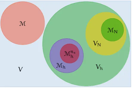
Notice that even if the snapshots belong toMnhs, the reduced basis functions do not longer belong toMnhs after they have been orthonormalized or gone through another kind of linear combination. Figure 1.1 gives an illustration of the set relations defined until now, note though, some interceptions between the sets could happen.
V
M
Vh
Mh
Mns
h
VN
MN
Figure 1.1: Reduced basis set relations
In order to implementVN in the computer we manipulate the snapshots in their discrete representation, i.e. using their coordinates in the basis ofVh, and not as real functions. Therefore, in practical matters,VN is never explicitly built but actually itsreduced basis matrix
UN:= [ζ1, . . . ,ζN]∈RNh×N
where forj=1, . . . , N, ζj = ζ (1) j , . . . , ζ
(Nh)
j
T
∈RNh
represents thej-th reduced basis function
ζj =
Nh
X
i=1 ζ(i)j ϕi,
with{ϕ1, . . . , ϕNh}
theVh basis.
There are two main algorithms to buildUN,greedyandproper orthogonal decomposition (POD). The main focus here will be on POD, for more information about greedy consult [83, 131]. Before showing the algorithm we present some preliminary definitions and minor results:
• LetXh be the matrix built with the scalar product ofV
whereϕi, i = 1, . . . , Nh, are the functions of the basis in Vh. Then we define the Xh scalar product andXh norm for allv,w∈RNh
by
(v,w)Xh :=vTXhw,
kvkXh :=pvTXhv.
TheXhnorm satisfies
kuhkXh =kuhkV (1.10)
whenuh ∈RNh represents the coordinates ofuh ∈Vh.
• Ifa(·,·;µ)is symmetric and coercive for allµ∈P, then
(v, w)µ:=a(v, w;µ), ∀v, w∈V,
and
kvkµ:=
q
(v, v)µ, ∀v∈V,
will denote the inner product and energy norm induced by the bilinear forma(·,·;µ). For bilinear forms independent ofµthe notation will be(·,·)a andk · ka.
• The reduced basis matrices considered afterwards will be orthonormal matricesUN ∈VN,
VN:={W∈RNh×N:WTW =IN},
or orthonormal with respect to theXh scalar product, i.e.UN∈VXNh for
VXh
N :={W∈R
Nh×N:WTX
hW=IN}.
Using the standardl2 scalar product
(v,w)2:=vTw, ∀v,w∈RNh,
then the orthogonal projection of x∈ RNh onto the span ofW = [w1, . . . ,wN]∈ VNis equal to
PWx=
N
X
j=1
(x,wj)2wj =WWTx.
Whereas ifW∈VXNh, theXhorthogonal projection onto its span correspond to
PXh
W x=
N
X
j=1
(x,wj)Xhwj =
N
X
j=1
wTjXhx wj=W
wT 1Xhx wT
2Xhx .. . wT
NXhx
In principle, the POD method builds UN using a truncated SVD representation of the
solution matrix
S:=u1|· · ·|uns
=uh(µ1)|· · ·|uh(µns)∈
RNh×ns,
which has in each column the discrete representationuh(µj) ={u(1)h (µj), . . . , u(Nh h)(µj)}T ∈RNh
of each snapshotuh(µj)∈Vh,
uh(µj) = Nh
X
i=1
u(i)h (µj)ϕi, j=1, . . . , ns.
To show how precise this method performs we use Schmidt-Eckart-Young theorem. This theorem gives an optimal approximation of a given matrix using sums of rank-1 matrices in thel2 normk · k2 and Frobenius normk · kF.
Theorem 2(Schmidt-Eckart-Young). LetA∈Rm×nbe a matrix of rankrwith SVD decomposition A=UΣZT,
where the left and right singular vectors are respectively
U=ζ1|· · ·|ζm
∈Rm×m, Z=Ψ1|· · ·|Ψn
∈Rn×n,
with singular values
Σ=diag(σ1, . . . , σp)∈Rm×n, σ1 ≥σ2≥. . .≥σp≥0, p=min(m, n).
Then for1≤k≤r, the matrix
Ak:= k
X
i=1
σiζiΨTi =UkUTkA, Uk=
ζ1|· · ·|ζk
,
satisfies
kA−Akk2 = min
B∈Rm×n
rank(B)≤k
kA−Bk2 =σk+1,
kA−AkkF= min
B∈Rm×n
rank(B)≤k
kA−BkF=
v u u t
r
X
i=k+1
σ2i. (1.12)
Proof. See [72].
Proposition 1. LetS=
u1|· · ·|uns
∈RNh×ns a solution matrix of rankrwith SVD
decomposi-tion
S=UΣZT,
where the left and right singular vectors are respectively
U=ζ1|· · ·|ζNh
∈RNh×Nh, Z=Ψ
1|· · ·|Ψns
∈Rns×ns,
with singular values
Σ=diag(σ1, . . . , σp)∈RNh×ns, σ1≥σ2≥. . .≥σp≥0, p=min(Nh, ns).
Then forN≤r,
UN=ζ1|· · ·|ζN
gives the following equality
ns
X
i=1
kui−PUNuik
2
2 = min
W∈VN
ns
X
i=1
kui−PWuik22 = r
X
i=N+1
σ2i. (1.13)
Proof. Proof from [131]. Taking in account thatkAk2 F=
P
ikaik22, whereai are the columns of Aresults
min
W∈VN
ns
X
i=1
kui−PWuik22= min
W∈VN
ns
X
i=1
kui−WWTuik22
= min
W∈VN
kS−WWTSkF.
Since rank(WWTS) =N, using Theorem 2 we achieve the minimum in the last equality when
WWTS=U NUTNS, so takingW=UNand using (1.12) yields equality (1.13).
In a analogous way we can prove a similar statement for theXh norm. Proposition 2. LetS=
u1|· · ·|uns
∈RNh×nsa solution matrix of rankrand
e
S=X1/2h S. Given the SVD decompositioneS=UeΣeZeT with left and right singular vectors
e
U=eζ1|· · ·|eζN
h
∈RNh×Nh,
e
Z=Ψe1|· · ·|Ψens
∈Rns×ns,
and singular values
e
Σ=diag(eσ1, . . . ,eσp)∈RNh×ns,
e
σ1≥eσ2≥. . .≥eσp≥0, p=min(Nh, ns).
the following equality holds forN≤randUN=X −1/2
h UeN=X
−1/2 h
e
ζ1|· · ·|eζN
,
ns
X
i=1
kui−PUXNhuik2Xh = min
W∈VXh N
ns
X
i=1
kui−PWXhuik2Xh =
r
X
i=N+1
e
Proof. Proof from [131]. Taking in account that with the symmetric matrix Xh,kX1/2h xk2 =
kxkXh for allx∈RXh,kAk2
F =
P
ikaik22, whereai are the columns of a matrixAand defining
e
W=X1/2h W, then
min
W∈VXh N
ns
X
i=1
kui−PXh
UNuik
2
Xh = min
W∈VXh N
ns
X
i=1
kui−WWTXhuik2X
h
= min
W∈VXh N
ns
X
i=1
kX1/2h ui−X1/2h WW TX1/2
h X 1/2 h uik22
= min
e
W∈VN
keS−WeWeTeSk2F.
Since rank(WeWeTeS) =N, by Theorem 2 the minimum in the last equality is achieved when
e
WWeTeS=UeNUeTNeS
so takingWe =UN, defininge UN=X
−1/2
h UNe and using (1.12) yields equality (1.14).
These results give a way to build the reduced basis matrixUNwith optimal representation of the solution matrix S thanks to (1.13) and (1.14), which at the same time are easy to implement and use. Nevertheless, note that they do not expose how the error behaves when
µ6∈Ξs. In this case, the usual way to compute error estimates is a-posteriori in the online stage.
Moreover, these propositions provide a way to select the dimension of the reduced basis which would be to pick the smallestNsuch that (1.13) or (1.14) is satisfied for a desirable errorε. Other practical way to selectNis to use what is calledrelative information contentof the POD basis [4], i.e. given a desirable errorε, pick the smallestNsuch that
I(N) :=
PN i=1σ2i
Pr i=1σ2i
≥1−ε2. (1.15)
The expressionI(N)consider the percentage of information retained inUNwith respect toS. In terms of Proposition 1 and 2, it means what percentage from the whole sum of singular values is held from the sum of their firstN. From here onwards we will callI(N)relative POD
errorto differentiate it from (1.13) and (1.14) that we will denote asPOD error. For both ways
to pickNapplies the same idea, the faster the decay of the singular values is, the smaller will beNfor attaining a prescribed error.
To summarize, POD method gives two possible procedures, we define them asPOD2and
PODXhrefering to Proposition 1 and 2 respectively, one which optimize thel2norm of the error and the other optimize theXhnorm instead. Their procedure follows as:
1. Construct the solution matrix S=
uh(µ1)|· · ·|uh(µns)
∈RNh×ns.
(1.16)
and make the transformationeS=X
1/2
2. For the l2 norm, compute the SVD decomposition of S and given an error tolerance ε, select the smallestNless or equal to the rank ofSsuch that the sum of the singular values satisfies one of these conditions,
r
X
i=N+1
σ2i ≤ε,
or P
N i=1σ2i
Pr i=1σ2i
≥1−ε2.
For theXh norm applies the same procedure but the SVD is computed toeS.
3. For thel2norm, constructUNtaking the firstNleft singular vectors ofSand for theXh norm caseUNis the result of multiplyingX−1/2h with the firstNleft singular vectors ofeS.
Once we finish these steps and store the reduced basis matrix we continue with the online stage to compute RB approximations. The following section explains in details the theorical results of this stage.
1.3
Reduced Basis Online Stage
There are two main ways to treat the online stage, one is usingGalerkin RB(G-RB) and the other isLeast-Square RB. The main focus will be the former because of the existence of optimal results for the problems in subsequent chapters.
The G-RB procedure is analogous to the usual Galerkin approach (1.7), but on the reduced basis space:
Givenµ∈P, finduN(µ)∈VNsuch that
a(uN(µ), vN;µ) =f(vN;µ) ∀vN∈VN. (1.17)
Equally as before, ifa(·,·;µ)is continuous and coercive inVandf(·;µ)is bounded inV, all these conditions satisfy in VN, thus (1.17) will have an unique solution in VN because of Lax-Milgram theorem. To find the RB solutionuN(µ)we solve a linear system like (1.5),
AN(µ)uN(µ) =fN(µ),
where its resulting vector
uN(µ) := (u(1)N (µ), . . . , u(N)N (µ))T
representsuN(µ),
uN(µ) =
N
X
i=1
u(i)N(µ)ζi.
Proposition 3. Ifa(·,·;µ) is symmetric and coercive for allµ ∈ P, then the solution of (1.17) satisfies
uN(µ) =argmin
v∈VN
kuh(µ) −vkµ, ∀µ∈P. (1.18)
Proof. Using theµ-orthogonality ofuh(µ) −uN(µ)inVNand the Cauchy-Schwarz inequality
kuh(µ) −uN(µ)k2
µ = a(uh(µ) −uN(µ), uh(µ) −uN(µ);µ)
= a(uh(µ) −uN(µ), uh(µ) −v;µ)
≤ kuh(µ) −uN(µ)kµkuh(µ) −vkµ, ∀v∈VN,
therefore,kuh(µ) −uN(µ)kµ≤ kuh(µ) −vkµfor allvinVN, proving thatuN(µ)is the desired minimum.
In the case of the normk · kV, there is also another classical optimal result. Furthermore, we add an original improvement that connects with POD in Proposition 2.
Proposition 4. Ifa(·,·;µ) is symmetric and coercive for allµ ∈ P, then the solution of (1.17) satisfies
kuh(µ) −uN(µ)kV ≤
γh(µ)
αN(µ)
1/2
inf v∈VN
kuh(µ) −vkV, ∀µ∈P, (1.19)
whereγh(µ)andαN(µ)are the continuity constant inVhand coercivity constant inVNofa(·,·;µ)
respectively. Moreover, ifµ∈ΞsandVN is generated by the POD reduced basis matrixUNbuilt in
Proposition 2, then
kuh(µ) −uN(µ)kV ≤
γh(µ)
αN(µ)
1/2 v u u t
r
X
i=N+1 σ2
i, µ∈Ξs, (1.20)
where σi, i = 1, . . . , r, are the singular values different from zero of the solution matrixSwith snapshotsuh(µ),µ∈Ξs.
Proof. As the bilinear forma(·,·;µ)is considered continuous and coercive inV, then there exist γh(µ)andαN(µ)such that
|a(u, v;µ)|≤γh(µ)kukVkvkV, ∀u, v∈Vh,
a(u, u;µ)≥αN(µ)kuk2V, ∀u∈VN.
Then using Proposition 3,
αN(µ)kuh(µ) −uN(µ)k2V ≤a(uh(µ) −uN(µ), uh(µ) −uN(µ);µ)
=kuh(µ) −uN(µ)k2µ
= min
v∈VN
a(uh(µ) −v, uh(µ) −v;µ)
≤γh(µ) inf
v∈VN
The expression (1.19) results from both extremes of the previous inequality, αN(µ)kuh(µ) −uN(µ)k2V ≤γh(µ) inf
v∈VN
kuh(µ) −vk2V. (1.21)
Now, supposeVNis generated by the reduced basis matrixUN ∈RNh×Ndefined in Propo-sition 2.
First note that even if the infimum at (1.21) is over the elements inVN,uh(µ)is in Vh. Therefore, to computekuh(µ) −vkV from a discrete point of view using the equivalent norm
k · kXh, it is necessary to change the coordinates ofv∈VN toVh, i.e.UNv∈R
Nh
withv ∈RN the coordinates of vinVN. Then, from the discrete representationuh(µ)ofuh(µ)inVh and (1.10) yields
inf v∈VN
kuh(µ) −vk2V = inf
v∈RN
kuh(µ) −UNvk2X
h, (1.22)
for which we obtain the infimum atv=UTNXhuh(µ)∈RN,
inf
v∈RN
kuh(µ) −UNvkX2h =kuh(µ) −UNU
T
NXhuh(µ)k2Xh. (1.23)
This is becauseUNUTNXhuh(µ) =P
Xh
UNuh(µ)which is the projection over the subspace generated
fromUN in the normk · kXh, see (1.11).
Letµ∈Ξs be an arbitrary parameter and denoteui = uh(µi), µi ∈Ξs fori=1, . . . , ns. In particular, there existsjsuch thatuj=uh(µ), then using (1.14) results
kuj−PUXhNujk2Xh ≤
ns
X
i=1
kui−PUXhNuik2Xh =
r
X
i=N+1
σ2i. (1.24)
From (1.21), (1.22), (1.23) and (1.24) we conclude that
αN(µ)kuh(µ) −uN(µ)k2V ≤γh(µ) r
X
i=N+1 σ2i
which gives the result (1.20).
An important case of (1.20) happens when the continuity and coercivity factor are bounded or as the case of the problems presented in Chapter 2 where the bilinear form is independent ofµ.
Corollary 1. Under the hypothesis of Proposition 4 suppose γh(µ) and αN(µ) are uniformly bounded above and below with boundsγ0andα0 respectively, then estimate (1.20) becomes
kuh(µ) −uN(µ)kV ≤
γ0 α0
1/2 v u u t
r
X
i=N+1 σ2
i, µ∈Ξs. (1.25)
in account the snapshots computed for building the reduced basis and it does not give any information whenµ6∈Ξs.
Another interesting fact from (1.20) is that if there exists high linear dependency between the solutions and therefore the rank ofSis small, then it is a good idea to takeN=r. From the projection point of view, (1.14) shows that perfect recovery of the original snapshots from the reduced basis can be achieved, and(1.20) exposes that G-RB procedure gives the possibility of recovering them with exact precision.
As explained before, Proposition 4 does not completely certify a good RB approximation for allµ∈P. A way to achieve it is to obtain an estimate of the supremum inPof (1.19),
sup µ∈P
kuh(µ) −uN(µ)kV ≤sup
µ∈P
"
γh(µ)
αN(µ)
1/2
inf v∈VN
kuh(µ) −vkV
#
. (1.26)
In general, knowing if a parametic problem isreducible, i.e. if there exists a small finite-dimesionalVNthat approximate all the elements of the computable solution manifoldMhwith an acceptable error, is a complicated task. Nevertheless, there are some results that takes in account the smoothness of the solution manifold and parametric complexity which give some conditions for reducibility. Section 1.4 and Section 1.5 go deeper in this subject.
1.4
Kolmogorov’s n-width Estimates
This section introduces an approach to estimate a-priori error bounds of reduced basis methods. The main idea behind it is to benchmark theKolmogorov’s n-width[99],
dn(M)V := inf
dim(Vn)=n
sup v∈Mwinf∈Vn
kv−wkV, (1.27)
using the smoothness and anisotropy of the solution manifold.
This quantity exposes the best possible accuracy in the norm ofV when approximating the elements ofM with linearn-dimensional spaces Vn. Its principal difference from (1.26) falls in the selection ofVn, i.e. Kolmogorovn-width ask for the best subspace of dimensionn while (1.26) has a fixed subspace built with POD. Even if (1.27) is not exactly (1.26), it gives an idea if it is possible to approximate the elements ofMuniformly from finite dimensional spaces.
The main result of this section is Theorem 6 which gives estimates for the Kolmogorov n-width. To arrive to its formulation and proof it is necessary to introduce some background first:
1. New formulation for the dependency of the parameters through a sequence of real num-bers.
2. Complex version of Lax-Milgram for the extension of the PDE to the complex domain.
The content of this section is based entirely in [53]. The main difference relies in the proof of Theorem 6, which is the same, but is presented in a straightforward manner. Moreover, this topic will be related to the construction of practical error estimators in Section 1.6.
The first important ingredient of this section is to identify the parametric part of the equation (1.6) through a sequence of real numbers. For example, consider a well defined operator equation
Au=f(µ),
wheref(µ)belongs to a subsetPof a Banach spaceXfor allµ∈P. The idea is to define a basis
(ψj)j≥1of functionsψj∈Xsuch that
f(µ) =f(y) =X
j≥1
yjψj, y:= (yj)j≥1, yj=yj(µ),
whereyj ∈ R,j ∈ N, and the series converges in theX-norm for eachµ ∈ P. The sequence
(yj)j≥1 is called anaffine representerofP.
The main advantage of affine representations is thatf(µ)can now be identified in a differ-ent way with the sequence(yj)j≥1. Therefore, for eachµ∈Pthere is one of this representers. If
Pis compact andyj(µ)continuous with respect toµ, then each functionψjcan be normalized such that
sup µ∈P|
yj(µ)|=1.
After normalization, each sequence(yj(µ))j≥1will belong to the infinite-dimensional cube Y := [−1, 1]N.
Two remarks are in hand, one is that taking a general sequence(yj)j≥1 fromYmay not
make the sum X
j≥1
yjψj (1.28)
necessarily converge inX. The affine representations that for every representer(yj)j≥1 ⊂Ythe sum (1.28) converges are calledcomplete. In this case, the sets
f(P) :={f(µ) :µ∈P},
f(Y) :=
f(y) =X
j≥1
yjψj : (yj)j≥1∈Y
,
satisfy the relationf(P)⊂f(Y).
The second remark is that could happen that for a specific sequence(yj)j≥1 there is no solutionu(y)and therefore the original equation is not well defined. If for each representer
(yj)j≥1 ⊂Ythere exists a solutionu(y), then the affine representation is calledcompatible. An important concept that helps estimate the Kolmogorovn-width is anisotropy. This regards to the fact that when kψjkX is small the scaled variableyj in Y have little influence on variations ofu(y)and therefore someyjhas more importance than others. This makes the
solution map
highly anisotropic.
Another relevant concept for obtaining an estimation of Kolmogorovn-width is the smooth-ness of the solution map. More concretely, in many cases it is possible to extend the solutions of a parametric problem to the complex domain in a holomorphic way. Next, we extend the theory of Section 1.1 to the complex valued case.
LetBbe the set of all sesquilinear forms defined inV×VandV0 the set of all antilinear functionals ofV. The norm ofb∈Bis defined as usual,
kbk:= sup
kvkV≤1,kwkV≤1
|b(v, w)|.
With these definitions we can consider the following problem: Givenb∈Bandf∈V0, findu∈V such that
b(u, v) =f(v), ∀v∈V. (1.30)
The existence and uniqueness of (1.30) can be obtained from a complex version of Lax-Milgram theorem, which is presented next.
LetL(V, W)be the space of all linear operatorsT from the Banach spaceVto the Banach spaceW with the norm
kTkL(V,W):=sup
v∈V
kTvkW
kvkV .
Givenb∈ B, the expressionb(u,·)is an antilinear functional and therefore, foru∈ V there existsBu∈V0 such that
b(u, v) = (Bu, v)V0,V, v∈V,
where(·,·)V0,V is the anti-dual pairing between VandV0. Hence,Bis a linear operator from V intoV0with
kBkL(V,V0)=kbk.
Consequently, the operatorBis continuous given the possibility to express the equation (1.30) in an equivalent operator equation inV0,
Bu=f. (1.31)
Theorem 3(Lax-Milgram). Letb∈Bbe a sequilinear form onV×Vsuch that it is coercive, i.e.
there existsα > 0such that
|b(u, u)|≥αkuk2V, ∀u∈V.
Then,Bin (1.31) is invertible and its inverse satisfies
kB−1kL(V0,V)≤ 1 α.
Therefore, for eachf∈V0, problem (1.30) has a unique solutionuf =B−1(f)which satisfies
kufkV ≤
Proof. See [132].
The procedure of the RB methods explained in previous sections looks for approximated solutions in the form of
(x,µ) uN(x,µ) =
N
X
i=1
u(i)N(µ)ζi(x),
whereζiare obtained from actual solutions of (1.6). In a more general context, the approxi-mated solutions of a parametric equation can be sought in theseparable form
(x,µ) un(x,µ) :=
n
X
i=1
vi(x)φi(µ),
wherevi ∈Vandφi :P→R, or equivalently,
(x, y) un(x, y) := n
X
i=1
vi(x)φi(y), (1.32)
withφi :Y→R.
The Kolmogorovn-width results we show later are obtained using approximations of the form (1.32) whenφis considered a polynomial, specifically a Legendre polynomial.
Assume the following notation for the sum in (1.32),
X
ν∈F
uνφν, (1.33)
whereFis a countable index,φν:Y →Randuν∈V.
Definition 1. A sequence(Λn)n≥1 of finite subsets ofFis called an exhaustion ofFif and only if,
for anyν∈F, there exists ann0such thatν∈Λnfor alln≥n0.
Definition 2. The series (1.33) converges conditionally with limituif and only if there exists an exhaustion(Λn)n≥1ofFsuch that
lim n→∞
u− X
ν∈Λn
uνφν
=0.
If the sum converges for every exhaustion(Λn)n≥1ofFthen is said to converge unconditionally. Certainly, having unconditional convergence is more desirable so later we can choose a convenient exhaustion(Λn)n≥1, i.e. the one that makes (1.33) converges the fastest tou. One useful result is the following classical fact from Hilbert space theory.
Theorem 4. Let (φν)ν∈F be an orthonormal basis ofL2(Y, ω) for some given measure ωon Y,
and letu∈L2(Y, V, ω). Then, the inner products
uν :=
Z
Y
are elements ofV, and the sum (1.33) converges unconditionally touinL2(Y, V, ω)with error
u− X
ν∈Λn
uνφν
L2(Y,V,ω)
= X
ν6∈Λn
kuνk2V
!1/2
,
for any exhaustion(Λn)n≥1.
Proof. See [100].
We introduce now the Legendre polynomials, assumeFthe set of all sequencesν= (νj)j≥1 of non-negative integers which are finitely supported and consider the separable sum
X
ν∈F
υνLν(y), Lν(y) =
Y
j≥1
Lνj(yj), (1.34)
where(Lk)k≥0is the sequence of Legendre polynomials on[−1, 1]
Qn(x) = 1 2nn!
dn dxn
h
(x2−1)n
i
,
normalized with respect to the uniform measure,
Z1
−1
|Qk(t)|2dt
2 =1.
It is known that Legendre polynomials are orthogonal on L2([−1, 1]) and therefore (Lk)k≥0 forms an orthonormal basis onL2(Y, ω)with
ω=⊗j≥1d yj 2 ,
the uniform measure overY. Using Theorem 4 the coefficientsυνare given by
υν:=
Z
Y
u(y)Lν(y)dω(y). (1.35)
For completing the proof of upcoming Theorem 6 will be convenient to have Legendre polyno-mials renormalized in the form of
X
ν∈F
wνPν(y), Pν(y) =
Y
j≥1
Pνj(yj),
where(Pk)k≥0 is the sequence of Legendre polynomials on[−1, 1]with the normalization
kPkkL∞([−1,1]) =Pk(0) =1.
The relationLk=
√
1+2kPkgives a way to compute the coefficientswν,
wν :=
Z
Y
u(y)Pν(y)dω(y) =Y
j≥1
(1+2νj)1/2υν. (1.36)
Lemma 2. Let p > 0,(cν)ν∈F ∈ lp(F) a sequence of positive numbers and(Λn)n≥1 the set of
indices that corresponds to thenlargestcν. Then, taking a real numberq > pyields
X
ν6∈Λν
cqν
!1/q
≤C(n+1)−s,
with constantsCandsequal to
C=k(cν)ν∈Fklp, s=
1 p−
1 q.
Proof. See [53].
Theorem 5. Consider a parametric problem of the form (1.6) such that it has a complete compatible affine representer with(ψj)j≥1 ∈ lp(N),p < 1, and that the solution mapu u(y) admits a
holomorphic extension to an open setOsuch that the parametersP(y)⊂Owith uniform bound
sup z∈O
ku(z)kV ≤C.
Then,(kwνkV)ν∈F ∈lp(F).
Proof. See [53].
Now we are ready to show the main result of this section. Some of the new findings of Section 1.5 and Section 1.6 are inspired by the ideas of its proof.
Theorem 6. If the parametric problem (1.6) satisfies the conditions of Theorem 5, then for each
p∈(0, 1),
dn(M)V ≤Cs(n+1)−s, n≥1, s:= 1
p−1. (1.37)
Proof. Proof from [53]. LetFbe the set of allυ= (υj)j≥1 of non-negative integers which are finitely supported, and computeυν as in (1.35),
υν=
Z
Y
u(y)Lν(y)dω(y).
From (1.36) results the coefficients of the normalized Legendre polynomialsPν
wν =Y
j≥1
(1+2νj)1/2υν,
and consequently the normalized Legendre series in the form of
X
ν∈F
wνPν. (1.38)
From Theorem 5 we know that
(kwνkV)ν∈F∈lp(F),
forp < 1. LetF∗⊂Fdenote the subset wherekwνkV ≤1, using the fact that the polynomials Pνare uniformly bounded by1yields
X
ν∈F∗ wνPν
L∞(Y,V)
=sup
y∈Y
X
ν∈F∗
wνPν(y)
V ≤ X
ν∈F∗
kwνkVsup y∈Y
|Pν(y)|≤
X
ν∈F∗
kwνkpV <∞,
and therefore the series (1.38) converges inL∞(Y, V). On the other hand, it also converges in L2(Y, V, ω)since
X
ν∈F
wνPν
L2(Y,V,ω)
≤ Z Y X
ν∈F
wνPν(y)
V
dω(y)≤
X
ν∈F∗ wνPν
L∞(Y,V)
Z
Y
dω(y) =
X
ν∈F∗ wνPν
L∞(Y,V) .
Taking in account thatuνis
uν= 1
kPνk2L2(Y,V,ω)
Z
Y
u(y)Pν(y)dω(y), ν∈F,
then Theorem 4 guarantees that in fact the Legendre series converges unconditionally touin L2(Y, V, ω), and consequently converges conditionally touinL∞(Y, V)for the trivial exhaustion (Fn)n≥1.
LetΛn be any exhaustion of F and suppose ε > 0is arbitrary. Also take m0 such that simultaneously satisfies
u− X
ν∈Fm
wνPν
L∞(Y,V)
≤ε/2,
X
ν6∈Fm
kwνkV ≤ε/2,
for m ≥ m0. Since(Λn)n≥1 is an exhaustion, there existsn0 such that Fm ⊂ Λn and conse-quently it yields
u− X
ν∈Λn
wνPν
L∞(Y,V)
≤
u− X
ν∈Fm
wνPν
L∞(Y,V)
+ X
ν6∈Fm
kwνkV ≤ε.
This proves that the series (1.38) converges unconditionally touin L∞(Y, V). Moreover, an estimation of the error comes from
u− X
ν∈Λn
wνPν
L∞(Y,V)
− X
ν6∈Λn
wνPν
L∞(Y,V)
≤
u− X
ν∈Λn
wνPν−
X
ν6∈Λn
wνPν
L∞(Y,V)
u− X
ν∈Λn
wνPν−
X
ν6∈Λn
wνPν
L∞(Y,V)
=
u−X
ν∈F
wνPnu
L∞(Y,V)
to conclude that
u− X
ν∈Λn
wνPν
L∞(Y,V)
≤
X
ν6∈Λn
wνPν
L∞(Y,V)
. (1.39)
Consider now Λn the set of indices of the n largest kwνkV and define the truncated Legendre expansion
un:=
X
ν∈Λn
wνPν.
Usingq=1in Lemma 2 the errorku−unkV reduce to
ku−unkV ≤ X
ν6∈Λn
wνPν≤C(n+1)1p−1,
withC=k(kwνkV)ν∈Fk.
Taking the definition of Kolmogorovn-width with the subspace Vn:=span{wν :ν∈Λn}⊂V,
gives the desired result through the inequalities
dn(M)V ≤sup v∈Mwinf∈Vn
kv−wkV ≤sup y∈Ywinf∈Vn
ku(y) −wkV ≤ ku−unkL∞(Y,V)≤C(n+1)
1 p−1.
There exists an ongoing research regarding Kolmogorovn-width bounds and exponential decay results (see [53, 125, 131] and their references) but many of them are sub-optimal in comparison to then-width spaces.
Unfortunaly, is not always possible to obtain good approximations from a linear space. The following new result shows a particular case of problems that cannot be approximated using RB methods. In particular, it will be useful in Chapter 2.
Theorem 7. Let the bilinear forma(·,·)be symmetric, coercive andµ-independent. Also suppose
VN=span{ζ1, . . . , ζN}=span{ζa1, . . . , ζaN},
where the elements ζai, i = 1, . . . , N, are obtained after an orthonormalization process of the original reduced basis functions with respect to the scalar product(·,·)a. If there exist a sequence
(µk)k≥1⊂Pand an indexi∈[N+1, Nh]such that an element of the orthogonal complement of VNinVh with respect to(·,·)a,
VNa =span{ζaN+1, . . . , ζaN
h},
satisfies|f(ζa
i;µk)|→ ∞whenk→ ∞, then
kuh(µk) −uN(µk)kV −−−→