Learning Financial Time Series for Prediction of the Stock Exchange Market

Learning Financial Time Series for Prediction

of the Stock Exchange Market

Roberto Rosas-Romero, Juan Pablo Medina-Ochoa

roberto.rosas@udlap.mx

Abstract

This paper presents the extension and application of three predictive models to time series within the financial sector, specifically data from 75 companies on the Mexican stock exchange market. A tool, which generates awareness of the potential benefits obtained from using formal financial services, would encourage more participation in a formal system. The three statistical models used for prediction of financial time series are a regression model, multi-layer perceptron with linear activation function at the output, and a Hidden Markov Model. Experiments were conducted by finding the optimal set of parameters for each predicting model while applying a model to 75 companies. Theory, issues, challenges and results related to the application of artificial predicting systems to financial time series, and performance of the methods are presented.

1

Introduction

Prediction is performed on time series within financial contexts, specifically the return of an individual stock from companies listed on the Mexican stock exchange market. The data to evaluate are the shares of 75 companies such as America Mobile, Coca-Cola, and Wal-Mart. The price of an individual stock is analyzed to predict changes that will happen so that a decision is taken.

According to data from a National Survey on Financial Inclusion in 2012 [1], Mexico is far behind in terms of the economically active population who invests in the stock market. It is important to bring formal saving systems to the people by working on systems that provide attractive yields with decreased risks. To perform an adequate forecasting analysis, historical prices, from companies listed in the stock exchange market, are obtained through sites like Yahoo! Finance [11].

The rest of the paper is organized as follows. Section 2 reviews related work that combines machine learning with financial engineering. Section 3 describes concepts of financial time series and how a predictive system is used to predict these signals. Section 4 gives an overview of the framework for each predictive model, specifically a regression model, a multi-layer perceptron and a Hidden Markov Model. Section 5 provides the experimental results. Conclusions are presented in Section 6.

Volume 58, 2019, Pages 418–427

2

Review of Related Work

In [2], a hybrid long-term and short-term evolutionary Trend Following (TF) algorithm is based on an eXtended Classifier System (XCS). TF investment strategies are combined so that long-term and short-term trends are integrated for evolution of the XCS. A proposed dynamic model shows returns from value stocks and growth stocks [3]. The effectiveness of local modeling in the prediction of time series is investigated in [4] with three classical forecasting methods, Neural Networks (NN), Adaptive Neuro-Fuzzy Inference System (ANFIS), and Least-Squares Support Vector Machine (LS-SVM). Experiments show that local modeling enhances performance for time series prediction. A technique for crash prediction based on the analysis of durations between subsequent crashes of the Dow Jones Industrial Average was developed in [5] where a significant autocorrelation in the series of durations between significant crashes suggests autoregressive conditional duration models (ACD) to forecast crashes. Artificial neural networks (ANN) are applied to trade financial time series by training and testing ANNs within stock market trading systems [6]. The forecasting performance of Bayesian Model Averaging (BMA) for a set of models of short-term rates was proposed by using weekly data for the one-month euro-dollar rate, BMA produces predictive likelihoods that are better than those associated with the majority of the short-rate models [7]. The problem of predicting the direction of movement of the price index in indian stock markets was studied by comparing four prediction models, Artificial Neural Networks (ANN), Support Vector Machines (SVM), Random Forest and naïve-Bayes [8].

3

Forecasting of Time Series

A financial time series is a sequence of observations, = , , … , , with features of some financial asset defined over discrete time, where the time index ( = 1, … , ) corresponds to an hour, or a trading day, or a month, etc. The price of an asset, , is an essential feature and given two consecutive daily prices, and , another financial feature, called return, is defined

where −1 ≤ . In our experiments, the daily stock price return , instead of price, is used as feature since it requires a smaller dynamic range which makes it easier to quantize. A positive return, > 0, represents an increase in the asset price while a negative return, < 0, means a price drop. Another feature is the gain which is given by = = 1 + . A positive return or price increase implies

a gain greater than one while a negative return or price drop introduces a gain less than one. Prediction of financial time series consists in estimating a future price return, , with trading days in advance by processing a set of past return observations , , … , _ℓ . The cumulative return price _!, after trading days, is given by the product of the initial asset price and the cumulative gain, _!= "1 + #"1 + # ∙∙∙ "1 + #. The return is also used as a performance metric of an artificial financial predictor. A financial predictor is efficient if it provides an investor with a higher cumulative gain than that obtained by not using it. Let us assume that a financial predictor has estimated four consecutive price return values according to the four-day sequence {increase, drop, increase, drop}. The consequence is that the investor decides to sell shares at days when a drop is expected, so that the return at those days is zero = 0 instead of negative, with a gain 1 + = 1. Therefore, the cumulative gain over the four-day period is "1 + #"1 + _%# which is higher than the original gain "1 + #"1 + #"1 + %#"1 + %#. A return gain curve shows the evolution of the return gain as time increases and the goal of an artificial financial predictor is to generate a return gain curve higher than the index curve. The higher the prediction accuracy the higher the obtained return.

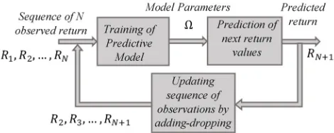
Prediction of financial time series is a two-stage periodic process where each cycle consists of: (1) training of the model to learn the parameters that maximize the probability of occurrence of an observation sequence of return values, (2) prediction of the return value for the upcoming trading day. Figure 1shows the two stages of a predictive model for financial time series

4

Predictive Models of Stock Market

4.1

Regression Model

A regression model establishes a relationship among a set of random variables [9]. In financial time series prediction, these random variables are price return values at multiple trading days. The model predicts a return value with days in advance to the current trading day. In a linear regression model, an input feature vector & = ' , , , … , _ℓ () ∈ +ℓ is applied to the model and the predicted return value is given by

∗ _{= -}) _&

ℓ , (2)

where ∗ is the estimated return value with trading days in advance, - = '., /₀, / , / , … , /ℓ () is the vector of regression parameters, including a term ., called bias. The feature vector & _ℓ = '1, , , , … , _ℓ () is extended to include a constant feature. The learning to estimate the unknown parameters is formulated as: (1) An observation sequence of price return values at trading days is generated 1 , , … , 2. (2) From the observation sequence, a training set 1"& , 3 #, "& , 3 #, … , "& ℓ , 3 ℓ #2 is generated. A training sample consists of one feature vector with ℓ consecutive price return values and the desired response which is the expected prediction with trading days in advance. (3) The training set is used to pose the set of equations & - = 4 by defining matrix & and vector 4 as

& = 5

⋯ ℓ 1

⋮ ⋮8 ⋱ ⋮ 1⋯ ℓ 1

ℓ ℓ ⋯ 1

:, 4 = 5 ℓ ℓ

⋮ :, (3)

(4) The parameters of the regression model are learned by applying Least-Squares Minimization (LSM), - = "&) &# &) 4.

4.2

Multi-Layer Perceptron with Linear Activation Function at the

Output

In the non-linear regression model there is a transformation of the observed return values previous to a combination. Another direction to follow, based on a transformation stage previous to a linear combination, is a multi-layer perceptron (MLP) where the transforming stage consists of hidden neurons. The action of hidden neurons is a mapping of the original feature space into a transformed feature space where the activation function for a hidden neuron is the logistic function. At each neuron

in the first hidden layer, -_; = <._;, /_;, , /_;, , … , /_{;,"ℓ #}, /_;,ℓ=)is the vector of synaptic weights, and & ℓ = '1, , , … , ℓ () is the feature vector. The output of a predictor takes values inside an infinite range and that is why the activation function for the output neuron is linear. The construction of the training set for the MLP follows the same process as the regression model according to equation 4. The training of the MLP-predictor is based on the back-propagation algorithm that adopts the gradient descent to iteratively update the synaptic weights according to the iterative step.

-;>" ?@# = -;>"AB3# − C _D-DE F

G, (4)

where H stands for the index of the layer, C is the learning rate, I = " ∗ − # is the squared error, ∗ is the return value estimated by the output neuron and is the real observed return value.

4.3

Prediction of Return Values based on Hidden Markov Models

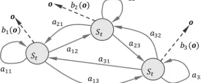
The Hidden Markov Model is a learning machine that is used to recognize sequential data [10]. The training stage is followed by prediction and this two-stage process is repeated so that the HMM dynamically updates its parameters to forecast future events according to dynamic trends of the market. At each cycle, the HMM is trained to predict a future return value based on past historic information by following a sequence of states J_K , J_K , J_K8, …. The transition from one state J = L to another J = M depends on a set conditional probabilities, called transition probabilities, defined as N = <O_P;= where O_P; = "J = M|J = L#; L, M = 1, … , S_T and S_T is the total number of possible states. At each state, the HMM emits an observation, which is a return value = , with a conditional probability, called emission probability, ._P" # = " |J = L#. The emission probability could be discrete or continuous. An example of the modelling of the variations of the return value of a stock from one trading day to another based on a HMM is illustrated in Figure 2. There are transitions from one state to another representing the change of stock states at different trading days. Each node in the graph represents a market state which is hidden. At each state, the observed return value depends on its emission probability function.

The emission function at each state might be a discrete probability function where the observed return value is discretized by assigning to it one of U possible symbols. In the discrete case, the emission probability is V = <._P;= where ._P;= " = M|J = L#; L = 1, … , S_T; M = 1, … , U. Using discrete emission probability functions simplifies modeling of the problem; however, a continuous emission probability density function (pdf) enables a more accurate problem. A general representation of a pdf for continuous observations associated with each state is given by a mixture of Gaussians (Rabbiner, 1989) according to

.P" # = W" |J = L# = X /PY Z" , [PY, \PY# ]

YK

; L = 1, … , ST; ^ = 1, … , U, (5)

component at state L, and /_PY is a mixture weight. The weights for the mixture of Gaussians are constrained to ∑]_YK /_PY = 1.

Training a HMM consists of estimating matrix N and the set of parameters {/_PY, [_PY, \_PY|L = 1, … , ST; ^ = 1, … , U}. The HMM receives a financial time series (sequence of observations) and the HMM parameters Ω (mixtures of Gaussians in combination with transition probabilities) are iteratively adjusted to find the optimum model by using the maximum likelihood method,

Ω = OHa max_e " , , … , , |Ω#, (6)

where is the length of the sequence, " , , … , , |Ω# is the cost function to be maximized, and Ω are the parameters of the model: (1) N = 1O_P;|L, M = 1, … , S_T2 and V = f._P;gL = 1, … , S_T; M = 1, … , U2 for discrete return values or, (2) 1/_PY, [_PY, \_PY|L = 1, … , S_T; ^ = 1, … , U2 for continuous return values. The parameters of the model are adjusted to estimate the model that maximizes " , … , | Ω# so that the model is optimum in terms of emitting the sequence of observed return values. An algorithm that maximizes the likelihood function is the Baum-Welch algorithm, which iteratively re-estimates the model. When the training of the HMM is done, it is possible to make a prediction for the next trading day. First, the most probable sequence of states for the observed return values is determined through the Viterbi algorithm, which finds the most likely state path by maximizing the joint probability function, h∗, … , h∗ = OHa max

T ,…,Ti " , … , , h , … , h |Ω#. The Viterbi algorithm determines the optimal path followed by a sequence of observed return values; however, for the case of predicting the return in the next coming trading days, the last state of the optimal path is the only state of interest. The most probable state for the next trading day h is determined by finding the most probable transition from the last state of the sequence, h O ? O ℎ? ?k lA^L a HO3L a 3Om = arg max_; OP;. The prediction for the next coming trading day corresponds to the most probable symbol at the predicted state h , WH?3Ll ?3 H? pH qOBp? hm^.AB = arg max_r .;r. For the case of continuous values, the return value at the predicted state h corresponds to the weighted average of the mean values of the Gaussian mixture WH?3Ll ?3 lA L pAph H? pH qOBp? = ∑]_YK l_;Y[_;Y. If the predicted return value is positive that means that the investor should buy or keep an investment; otherwise, the investor should sell. After each prediction, the HMM is trained again to obtain a new prediction by applying the add-drop process to the observed sequence where the newest return value is added and the oldest observed value is dropped. The prediction process is carried out with the training alternatively. This is what market analysts do.

5

Experimental Results

5.1

Data Set

5.2

Regression Model Results

The first set of experiments includes regression results. We different sets of parameters. In this set of experiments, (1) for each prediction the length of the observation sequence is adjusted from 30 to 530 trading days in increments of 50 days, (2) the predictive model is applied on the training data with different polynomial order values (H = 1, 2, 3), and (3) considered (ℓ = 3, 4, 5, 6). A total of 120 different combinations for the model parameter values were tried to find the optimal set of parameters, 1 ∗_{, H}∗_{, ℓ}∗_{2. The goal of an artificial predictor is to make the most accurate predictions, which result in} a cumulative return gain curve higher than the curve provided by the market. It is considered that one monetary unit is the input to the predicting analysis. Results show that the regression model performs better than the market in terms of the final return gain. Figure 3 shows an example of the optimal prediction achieved by the regression model when it is applied to analyze the shares of ICA Inc. (civil engineering) over 3,548 days. It is observed that the cumulative gain of the predicting system (orange) exceeds that of the market (blue). This case corresponds to a linear regression model (first order polynomial) where return values over a four-day period are used as features to predict the return for tomorrow.

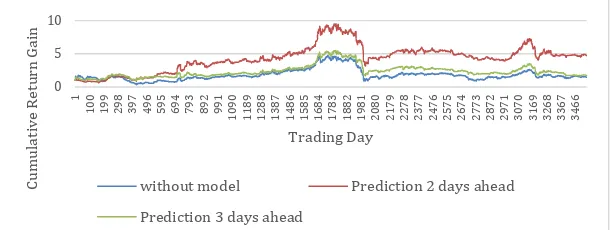
The same model is used to predict the return gain with 2 and 3 days in advance over 3,548 days of the stock return at ICA in Figure 4. Results show that the regression model still performs above the market; however, the performance degrades as the number of days to predict in advance is increased.

There are results that are very promising to investors where the predicted return reaches extremely high values. We have the case where the regression model was tested with the stock price of Liverpool Inc. (shopping centers, department stores) where the cumulative gain at the end of 10 years is 1659577456. Non-linear regression can follow non-linear trends of return values; however, non-linear behavior is not easily found in all series. A regression model achieved the best prediction in 36 out of the 64 companies listed.

Figure 3: Cumulative return gain obtained by a regression model vs. the curve generated by the market.

-4 1 6 11 16 21 1 1 1 2 2 2 3 3 3 4 4 4 5 5 5 6 6 6 7 7 7 8 8 8 9 1 0 0 0 1 1 1 1 1 2 2 2 1 3 3 3 1 4 4 4 1 5 5 5 1 6 6 6 1 7 7 7 1 8 8 8 1 9 9 9 2 1 1 0 2 2 2 1 2 3 3 2 2 4 4 3 2 5 5 4 2 6 6 5 2 7 7 6 2 8 8 7 2 9 9 8 3 1 0 9 3 2 2 0 3 3 3 1 3 4 4 2 C um ul a ti v e R e tur n G a in Trading Day

Without Model Non-linear regression

Figure 4: Predicting the cumulative return gain with 2 and 3 days in advance by using a regression model. . 0 5 10 1 1 0 0 1 9 9 2 9 8 3 9 7 4 9 6 5 9 5 6 9 4 7 9 3 8 9 2 9 9 1 1 0 9 0 1 1 8 9 1 2 8 8 1 3 8 7 1 4 8 6 1 5 8 5 1 6 8 4 1 7 8 3 1 8 8 2 1 9 8 1 2 0 8 0 2 1 7 9 2 2 7 8 2 3 7 7 2 4 7 6 2 5 7 5 2 6 7 4 2 7 7 3 2 8 7 2 2 9 7 1 3 0 7 0 3 1 6 9 3 2 6 8 3 3 6 7 3 4 6 6 C um ul a ti v e R e tur n G a in Trading Day

without model Prediction 2 days ahead

Figure 5 shows a comparison between (1) the cumulative return gain by following a regression model (orange column) and (2) the return provided by the market (blue column) for 42 companies.

5.3

Multi-Layer Perceptron Results

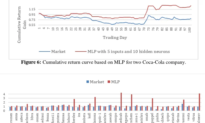
Experiments were run to predict the return value over 100 trading days for each company by using a one-hidden-layer MLP with a linear activation function at the output. For each company, 15 different sets of parameters were tried. The number of features (from 3 to 7) and the number of hidden neurons (from 10 to 20 in increments of 5) were adjusted. At each predicted day, one MLP is trained by using a training sequence of 150 past return values and a learning rate of 0.3. One example is depicted in Figure 6. The company under study is Coca-Cola where where the best parameters correspond to 5 inputs and 10 hidden neurons. Figure 7 compares the cumulative gain provided by the market with that generated by the MLP model at the end of 100 days for 37 companies.

Figure 5: Comparing the cumulative return gain estimated by a predictive model vs. the cumulative return gain provided by the market for 42 companies.

0 10 20 30 40 50 60 la la b m 5 tr a ci sh rs m a x co m cp o g sa n b o rb -1 h ci

ty _ica

ie n o v a v it ro a v o la ra w a lm e x v v a sc o n i v e st a a u tl a n b a x te lc p o a z te c a cp

o _ac

a ct in v rb a e ro m e x a lp e k a a m x l a n g e ld 1 0 a ra b im b o a b o ls a a b b v a d ia b lo i1 0 d a n h o s1 3 g e n te ra g fa m sa a g fi n b u ro g a p b g b m o g ca rs o a 1 sp o rt s te a k cp o te rr a 1 3 tl e v is a cp o p o ch te cb q cc p o sa n sa re b so ri a n a b

Market Predictive Model

Figure 6: Cumulative return curve based on MLP for two Coca-Cola company.

0.55 0.75 0.95 1.15

1 4 7

1 0 1 3 1 6 1 9 2 2 2 5 2 8 3 1 3 4 3 7 4 0 4 3 4 6 4 9 5 2 5 5 5 8 6 1 6 4 6 7 7 0 7 3 7 6 7 9 8 2 8 5 8 8 9 1 9 4 9 7 1 0 0 C um ul a ti v e R e tur n G a in Trading Day

Market MLP with 5 inputs and 10 hidden neurons

Figure 7: Comparison of the cumulative return gain estimated by an MLP vs. the cumulative return gain by the market for 37 companies at the end of a 100-day period.

5.4

Hidden Markov Model Results

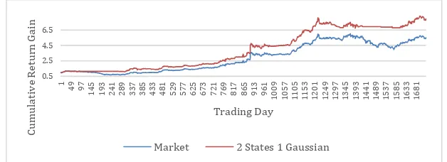
Cumulative return gain curves corresponding to the market and the predicting system are shown in Figure 8. Tthe artificial predictor beats the market at each trading day. The final cumulative return gain provided by the predicting system is 7.9509 vs. a return of 5.5094 generated by the market. The computational time for this experiment takes multiple hours in a MATLAB implementation running on an Intel Core 5 processor at 2.5 GHz since15 HMMs were trained at each predicted day. Thus, the total number of trained HMMs in this particular experiment was 25,905.

All the companies were analyzed to predict the return over 100 trading days. The model is applied on the training data with different values for the model parameters: the length of the training sequence ( = 150), the number of states (3 ≤ S_T ≤ 5), and the number of Gaussians (3 ≤ U ≤ 4). Six sets of parameters were used to analyze each company.

5.5

Comparison of Predictive Models

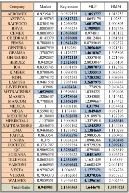
Three predictive models (regression, MLP, HMM) were tested under the same conditions to determine the best model. Each model was applied to predict the return of a company over 100 trading days. Each model was trained with a sequence of 150 return values. Table 1 shows the final return gain generated by each model as well as by the market for the case of 35 companies. The optimal set of parameters for each model was determined by trying different parameter value combinations. For the case of the regression model, the parameters to change are the regression order H and the number of input return values ℓ. For the MLP, the parameters to adjust are the number of hidden neurons x and the number of input return values ℓ. Finally, the HMM was adjusted by varying the number of states ST and the number of Gaussians U. The secondcolumn of Table 1 contains the final cumulative gain for each company without using a predicting system. The last row of the second column contains the average gain provided by the market, which is 0.945981 and represents a loss of 5.40% of the initial investment. This loss implies the need for using predicting systems. Other columns contain the net gain provided by each predictive model. There is one company for which no model overcomes the market. Even though the MLP reaches the highest gain for the most companies, the regression model is the predictor with the highest overall gain of 2.1330363as in the last row of Table 1. The overall gain obtained by the combination of the three models is 2.2631854. The overall returns generated by the regression model, MLP and HMM are 113.3%, 64.47%, 35.51%, respectively; while the return generated by the market is -5.40%. The combination of the three models generates a return of 133.30%. Even though the HMM has the worst performance of all predictive models, it still beats the market and provides a gain greater than one.

Figure 8: Cumulative return gain curve obtained by following a HMM vs. the curve generated by the market.

0.5 2.5 4.5 6.5

1

4

9

9

7

1

4

5

1

9

3

2

4

1

2

8

9

3

3

7

3

8

5

4

3

3

4

8

1

5

2

9

5

7

7

6

2

5

6

7

3

7

2

1

7

6

9

8

1

7

8

6

5

9

1

3

9

6

1

1

0

0

9

1

0

5

7

1

1

0

5

1

1

5

3

1

2

0

1

1

2

4

9

1

2

9

7

1

3

4

5

1

3

9

3

1

4

4

1

1

4

8

9

1

5

3

7

1

5

8

5

1

6

3

3

1

6

8

1

C

um

ul

a

ti

v

e

R

e

tur

n

G

a

in

Trading Day

Table 1: Cumulative gain generated by the market and each predictive model. The highest gain values are highlighted.

6

Conclusions

It is possible to predict the Mexican stock exchange market behavior and thereby obtain better returns than those without an artificial predictor. The optimal parameters and model depend on the company and its financial background. The greater the number of days to be predicted in advance, the higher the error. Predicting just one day in advance gives the best results.

This work presents the extension, application, and comparison of three predictive models (regression model, multi-layer perceptron, hidden Markov model) to financial time series. It was found that (1) the overall return gain generated by any predictive model exceeds the gain generated by the market, (2) the MLP is the model that reaches the highest gain for the most companies while the regression model is the predictor that generates the highest overall gain, (3) the overall gain is

Company Market Regression MLP HMM AEROMEX 0.9235412 0.9897535 1.1053777 1.018253

AZTECA 1.0195783 1.0817322 1.0653179 1.0283 BACHOCO 0.8304196 1.2960078 1.6015768 1.004805

BBVA 1.0805037 1.0546254 1.1989851 1.167358 CEMEX 0.8003953 1.0603605 0.974811 1.013132 CHEDRAUI 1.0143379 1.0876008 1.0812484 1.061681 FEMSA 0.7088816 1.0842429 0.8755645 1.072522 GENTERA 0.8607939 1.169289 1.3056469 0.921314 GFAMSA 1.3780793 1.4176272 1.4610367 1.305896 GFINBURO 1.0292887 1.3572115 1.3557048 1.271499 HERDEZ 0.942029 5.2323601 2.8033047 2.736104 ICA 0.8335745 1.0301159 1.3887073 1.112567 KIMBER 0.8700696 1.0990678 1.1355513 1.088633 KOFL 1.3874172 1.0675243 1.7203202 1.408948 LAMOSA 0.9461538 2.7965148 3.2687975 0.834843 LIVERPOOL 1.183908 4.402424 1.1774928 2.940424 M5TRACISHRS 1.0529891 1.0396601 1.0354221 1.039406 MASECA 1.3206107 2.8578046 1.3543001 1.414612 MAXCOM 0.7708831 1.3568249 1.2399667 1.134425 MEDICA 1 1.4808116 4.31794 1.034461 MEGA 0.5590102 1.137416 1.1849469 0.987195 MEXCHEM 1.0138889 14.502678 3.9189978 3.127296 MFRISCOA-1 1.1137009 1.3000803 1.3374918 1.483616

NAFTRACISHRS 1.0546075 1.0667162 1.1543293 1.144488 OMA 0.9468685 1.1277492 1.1384669 1.110289 PAPPEL 0.863354 6.4805576 2.9883536 1.860465 PINFRA 0.375 1.0884254 1.0986366 1.343496

POCHTEC 0.3731707 0.6889354 0.9729226 1.399212

QC 0.9869226 1.3788467 1.0795881 1.028819 SORIANA 0.5996578 0.9307625 1.0451693 0.896578 TELEVISA 0.8683435 1.2354889 1.1631439 1.05859

VASCONI 1.6460905 3.8909642 2.6602429 2.045167 VESTA 0.9758745 1.004862 1.1777171 0.974726 VITROA 0.7934373 0.9162661 1.0370356 0.955873 WALMEX 0.9859551 3.9449612 4.1396161 2.402544

maximized through the combination of the three models, (4) the HMM is the model with the worst performance; however, it still beats the performance of the market and provides a return gain greater than one.

References

[1] Peevey. National survey of financial inclusion. http://socialprotectionet.org/resources/national-financial-inclusion-survey-2012-enif-2012, 2013.

[2] Y. Hu, B. Feng, X. Zhang, E. W. T. Ngai, M. Liu. Stock trading rule with an evolutionary trend following model. Expert Systems with Applications, 42: 212-222, 2015.

[3] I. C. Yeh, T. K. Hsu. Exploring the dynamic model of the returns from value stocks and growth stocks using time series mining. Expert Systems with Applications, 41: 7730-7743, 2014.

[4] S. F. Wu, S. J. Lee. Employing local modeling in machine learning methods for time series predictions. Expert Systems with Applications, 42: 342-354, 2015.

[5] V. Pyrlik. Autoregressive conditional duration as a model for financial market crashes prediction. Physica A, 392: 6041-6051, 2013.

[6] B. Vanstone, G. Finnie. Enhancing stock market performance with ANNs. Expert Systems with Applications, 37: 6602-6620, 2010.

[7] C. L. Chua, S. Suardy and S. Tsiaplias. Predicting short-term interest rates using Bayesian model averaging: Evidence from weekly and high frequency data. International Journal of Forecasting, vol. 29: 442-455, 2013.

[8] J. Patel, S. Shah, P. Thakkar, K. Kotecha. Predicting stock and stock price index movement using trend deterministic data preparation and machine learning techniques. Expert Systems with Applications, 42: 259-268, 2015.

[9] S. Theodoridis, K. Koutrombas. Pattern Recognition. Elsevier, 2009.

[10] L. H. Rabiner. A tutorial on hidden Markov models and selected applications in speech processing. In Proceedings of the IEEE, 77(2): 257-286, 1989.