Generalized Degree Distance of Strong Product of Graphs

(1)

Vol. 10, No. 2 (2015), pp 87-98 DOI: 10.7508/ijmsi.2015.02.009

Generalized Degree Distance of Strong Product of Graphs

K. Pattabiraman∗_{, P. Kandan}

Department of Mathematics, Annamalai University, Annamalainagar 608 002, India.

E-mail: pramank@gmail.com E-mail: kandan2k@gmail.com

Abstract. In this paper, the exact formulae for the generalized degree distance, degree distance and reciprocal degree distance of strong product of a connected and the complete multipartite graph with partite sets of sizesm0, m1, . . . , mr−1 are obtained. Using the results obtained here, the formulae for the degree distance and reciprocal degree distance of the closed and open fence graphs are computed.

Keywords: Generalized degree distance, Degree distance, Reciprocal degree distance, Strong product.

2000 Mathematics subject classification: 05C12, 05C76. 1. Introduction

All the graphs considered in this paper are simple and connected. For ver-tices u, v ∈ V(G), the distance between u and v in G, denoted by dG(u, v),

is the length of a shortest (u, v)-path in G and let dG(v) be the degree of a

vertexv∈V(G).Thestrong productof graphsGandH,denoted byG⊠H,is the graph with vertex setV(G)×V(H) ={(u, v) :u∈V(G), v∈V(H)} and (u, x)(v, y) is an edge whenever (i)u=v andxy ∈E(H), or (ii)uv ∈E(G) andx=y,or (iii)uv∈E(G) andxy∈E(H),see Fig.1.

∗_{Corresponding Author}

Received 22 July 2014; Accepted 27 December 2014 c

2015 Academic Center for Education, Culture and Research TMU

87

(2)

b

C3⊠P3

Fig. 1. Strong product ofC3andP3.

Atopological indexof a graph is a real number related to the graph; it does not depend on labeling or pictorial representation of a graph. In theoretical chemistry, molecular structure descriptors (also called topological indices) are used for modelling physicochemical, pharmacologic, toxicologic, biological and other properties of chemical compounds [8]. There exist several types of such indices, especially those based on vertex and edge distances. One of the most intensively studied topological indices is the Weiner index.

Let G be a connected graph. Then W iener index of G is defined as

W(G) = 1 2

P

u, v∈V(G)

dG(u, v) with the summation going over all pairs of

dis-tinct vertices ofG. This definition can be further generalized in the following way:

Wλ(G) = 12

P

u, v∈V(G)

dλ

G(u, v), where dλG(u, v) = (dG(u, v))λ and λ is a real

number [9, 10]. Ifλ=−1,thenW−1(G) =H(G),whereH(G) is Harary index of G. In the chemical literature also W1

2 [27] as well as the general case Wλ were examined [6, 11]. Wiener index of 2-dimensional square and comb lattices with open ends is obtained by Graovac et al. in [5]. In [17] the Wiener in-dex of HAC5C7[p, q] and HAC5C6C7[p, q] nanotubes are computed by using GAP program. Dobrynin and Kochetova [4] and Gutman [7] independently proposed a vertex-degree-weighted version of Wiener index called degree dis-tanceor Schultz molecular topological index, which is defined for a connected graphGas

DD(G) = 1 2

P

u,v∈V(G)

(dG(u) +dG(v))dG(u, v),wheredG(u) is the degree of the

vertex uin G.Note that the degree distance is a degree-weight version of the Wiener index. In the literature, many results on the degree distanceDD(G) have been put forward in past decades and they mainly deal with extreme properties of DD(G). Tomescu[24] showed that the star is the unique graph with minimum degree distance within the class onn-vertex connected graphs. Tomescu[25] deduced properties od graphs with minimum degree distance in

(3)

the class ofn-vertex connected graphs withm≥n−1 edges. For other related results along this line, see [2, 14, 18].

Additively weighted Harary index(HA) or reciprocal degree distance(RDD)

is defined in [1] as HA(G) = RDD(G) = 12

P

u,v∈V(G)

(dG(u)+dG(v))

dG(u,v) . In [12],

Hamzeh et. al recently introduced generalized degree distance of graphs. Hua and Zhang [15] have obtained lower and upper bounds for the reciprocal gree distance of graph in terms of other graph invariants including the de-gree distance, Harary index, the first Zagreb index, the first Zagreb coindex, pendent vertices, independence number, chromatic number and vertex-, and edge-connectivity. Pattabiraman and Vijayaragavan [21, 22] have obtained the reciprocal degree distance of join, tensor product, strong product and wreath product of two connected graphs in terms of other graph invariants. The chem-ical applications and mathematchem-ical properties of the reciprocal degree distance are well studied in [1, 19, 23].

The generalized degree distance, denoted byHλ(G),is defined as Hλ(G) = 12

P

u,v∈V(G)

(dG(u) +dG(v))dλG(u, v), where λ is a any real number.

If λ = 1, then Hλ(G) = DD(G) and if λ = −1, then Hλ(G) = RDD(G).

The generalized degree distance of unicyclic and bicyclic graphs are studied by Hamzeh et. al [12, 13]. Also they are given the generalized degree distance of Cartesian product, join, symmetric difference, composition and disjunction of two graphs. It is well known that many graphs arise from simpler graphs via various graph operations. Hence it is important to understand how certain invariants of such product graphs are related to the corresponding invariants of the original graphs. In this paper, the exact formulae for the generalized degree distance, degree distance and reciprocal degree distance of strong productG⊠

Km0, m1, ..., mr−1,whereKm0, m1, ..., mr−1is the complete multipartite graph with partite sets of sizesm0, m1, . . . , mr−1are obtained.

Thefirst Zagreb indexis defined asM1(G) = P

u∈V(G)

dG(u)2.In fact, one can

rewrite the first Zagreb index asM1(G) = P

uv∈E(G)

(dG(u) +dG(v)).The Zagreb

indices are found to have applications in QSPR and QSAR studies as well, see [3].

Ifm0=m1=. . .=mr−1=sinKm0, m1, ..., mr−1 (the complete multipartite graph with partite sets of sizesm0, m1, . . . , mr−1), then we denote it byKr(s). ForS ⊆V(G), hSidenotes the subgraph ofGinduced by S. For two subsets

S, T ⊂ V(G), not necessarily disjoint, by dG(S, T), we mean the sum of the

distances inGfrom each vertex ofS to every vertex ofT,that is,dG(S, T) = P

s∈S, t∈T

dG(s, t).

(4)

2. Generalized Degree Distance of Strong Product of Graphs In this section, we obtain the generalized degree distance ofG⊠Km0, m1, ..., mr−1. Let G be a simple connected graph with V(G) = {v0, v1, . . . , vn−1} and let

Km0, m1, ..., mr−1, r ≥2, be the complete multiparite graph with partite sets

V0, V1, . . . , Vr−1and let|Vi|=mi, 0≤i≤r−1.In the graphG⊠Km0, m1, ..., mr−1, let Bij =vi×Vj, vi ∈ V(G) and 0 ≤ j ≤r−1. For our convenience, as in

the case of tensor product, the vertex set ofG⊠Km0, m1, ..., mr−1 is written as

V(G)×V(Km0, m1, ..., mr−1) =

r−1

n−1

S

i= 0

j= 0

Bij.As in the tensor product of graphs, let

B₌_{_B_ij_}_i_{= 0}_,₁_{,..., n}₋₁

j= 0,1,..., r−1. LetXi=

r−1

S

j= 0

Bij andYj= n−1

S

i= 0

Bij; we callXi andYj

aslayerandcolumnofG⊠Km0, m1, ..., mr−1,respectively, see Figures 2 and 3. If we denoteV(Bij) ={xi1, xi2, . . . , ximj}andV(Bkp) ={xk1, xk2, . . . , xk mp},

then xiℓ and xkℓ,1 ≤ ℓ ≤ j, are called the corresponding vertices of Bij

and Bkp. Further, if vivk ∈ E(G), then the induced subgraph hBijSBkpi

of G⊠Km0, m1, ..., mr−1 is isomorphic to K|Vj||Vp| or, mp independent edges

joining the corresponding vertices of Bij and Bkj according asj6=porj =p,

respectively.

v0

V

er

ti

ce

s

o

f

G

Vertices ofKm0, m1, ..., mr−1

vi

v1

vk+1

vn−1

V0 Vj Vp Vr−1

Bkj

vℓ

vk

V1

b

B00 B01 B0(r−1)

Bi0 Bi1 Bi(r−1)

Bij

B(n−1)0 B(n−1)1 B(n−1)(r−1)

Structure of shortest paths inG_⊠K_m

0, m1, ..., mr−1corresponding to an edge inG.

b

xiℓ

xkℓ

Fig. 2.

Ifvivk ∈ E(G),then shortest paths of length 1 and 2 from Bij toBkj are

shown in solid edges, where the vertical line between Bij and Bkj denotes

the edge joining the corresponding vertices of Bij andBkj. The broken edges

denote a shortest path of length 2 from a vertex ofBij to a vertex ofBij.

The proof of the following lemma follows easily from the properties and structure ofG⊠Km0, m1, ..., mr−1,see Figs. 2 and 3.

(5)

Lemma 2.1. Let G be a connected graph and letBij, Bkp ∈B of the graph G′=G⊠Km0, m1, ..., mr−1, wherer≥2.

(i)If vivk ∈E(G) andxit∈Bij, xkℓ∈Bkj, then

dG′(x_it, x_kℓ) = (

1, ift=ℓ,

2, ift6=ℓ,

and if xit∈Bij, xkℓ∈Bkp, j=6 p,thendG′(x_it, x_kℓ) = 1.

(ii)Ifvivk ∈/E(G),then for any two verticesxit∈Bij, xkℓ∈Bkp, dG′(x_it, x_kℓ) = dG(vi, vk).

(iii)For any two distinct vertices in Bij,their distance is 2.

The proof of the following lemma follows easily from Lemma 2.1. The lemma is used in the proof of the main theorems of this section.

Lemma 2.2. Let G be a connected graph and letBij, Bkp ∈B of the graph G′₌_G_⊠_K

m0, m1, ..., mr−1, wherer≥2. (i)If vivk ∈E(G), then

dλG′(B_ij, B_kp) = (

mjmp, if j6=p,

(1−2λ₍_m

j−1))mj, ifj =p.

(ii)If vivk ∈/E(G), thendλG′(Bij, Bkp) = (

mjmpdλG(vi, vk), if j6=p, m2

jdλG(vi, vk), if j=p.

(iii)dλ

G′(Bij, Bip) = (

mjmp, if j6=p,

2λ_m

j(mj−1), if j=p.

v0

V

er

ti

ce

s

o

f

G

Vertices ofKm0, m1, ..., mr−1

vi+1

v1

vk

vn−1

V0 Vj Vp Vr−1

Bkj

Bij

vi

vk−1

V1

vi+2

b

B01

B00 B0(r−1)

Bi0 Bi1 Bi(r−1)

B(n−1)0 B(n−1)1 B(n−1)(r−1)

b

Bkp

Fig. 3.

Corresponding to a shortest path of length k > 1 in G, the shortest path from any vertex of Bij to any vertex ofBkj (resp. any vertex of Bij to any

(6)

vertex of

Bkp, p6=j) of lenght kis shown in solid edges (resp. broken edges).

Lemma 2.3. LetGbe a connected graph and letBij inG′ =G⊠Km0, m1, ..., mr−1. Then the degree of a vertex(vi, uj)∈Bij inG′ isdG′((v_i, u_j)) =d_G(v_i)+(n₀− mj) +dG(vi)(n0−mj), wheren0=

r−1

P

j=0

mj.

Remark 2.4. The sumsPrj, p−1= 0

j6=p

mjmp= 2q, r−1

P

j=0

m2

j =n20−2q,

Pr−1

j, p= 0

j6=p m2

jmp= n3

0−2n0q−

r−1

P

j=0

m3

j = Pr−1

j, p= 0

j6=p

mjm2pand Pr−1

j, p= 0

j6=p m3

jmp=n0

r−1

P

j=0

m3

j− r−1

P

j=0

m4

j = Pr−1

j, p= 0

j6=p

mjm3p,wheren0=

r−1

P

j=0

mjandqis the number of edges ofKm0, m1, ..., mr−1.

Theorem 2.5. LetGbe a connected graph withnvertices andmedges. Then

Hλ(G⊠Km0, m1, ..., mr−1) = (n

2

0 + 2n0q)Hλ(G) + 4n0qWλ(G) +M1(G)(1− 2λ₎₂_qn

0−n30−n20+n0+ 4q+

r−1

P

j=0

m3

j

+m4qn0(3−2λ+1)−2n30(2−2λ+1) + 4q(2−2λ₋₂λ+1_{) +}_n

0(n0−1)2λ+1+ 2(2−2λ+1)

r−1

P

j=0

m3

j

+n2n0q(2−2λ) +

n3

0(2λ−1)−2λ+1q+ (1−2λ)

r−1

P

j=0

m3

j

, r≥2.

Proof. LetG′ ₌_G_⊠_K

m0, m1, ..., mr−1.Clearly,

Hλ(G

′

) = 1

2

X

Bij, Bkp∈B

dG′(Bij) +dG′(B_kp)

dλG′(Bij, Bkp)

= 1

2

n−1

X

i= 0

r−1

X

j, p= 0

j6=p

dG′(Bij) +dG′(Bip)

dλG′(Bij, Bip)

+

n−1

X

i, k= 0

i6=k r−1

X

j= 0

dG′(Bij) +dG′(Bkj)

dλG′(Bij, Bkj)

+

n−1

X

i, k= 0

i6=k r−1

X

j, p= 0

j6=p

dG′(Bij) +dG′(Bkp)

dλG′(Bij, Bkp)

+

n−1

X

i= 0

r−1

X

j= 0

dG′(Bij) +dG′(Bij)

dλG′(Bij, Bij)

!

= 1

2{A1+A2+A3+A4}, (2.1)

where A1, A2, A3 andA4 are the sums of the terms of the above expression, in order.

(7)

We shall obtainA1 toA4of (2.1),separately.

A1 =

n−1

X

i=0

r−1

X

j, p= 0

j6=p

dG′(Bij) +dG′(Bip)

dλG′(Bij, Bip)

=

n−1

X

i=0

r−1

X

j, p= 0

j6=p

2dG(vi) +dG(vi)(2n0−mj−mp) + (2n0−mj−mp)

mjmp,

by Lemmas 2.2 and 2.3

= 8mq+ 2m4n0q−2(n30−2n0q−

r−1

X

j=0

m3j)

+n4n0q−2(n30−2n0q−

r−1

X

j=0

m3j)

,

by Remark 2.4

= 2m4q+ 8n0q−2n30+ 2

r−1

X

j=0

m3j

+n8n0q−2n30+ 2

r−1

X

j=0

m3j

.

A2 =

r−1

X

j= 0

n−1

X

i, k= 0

i6=k

dG′(Bij) +dG′(Bkj)

dλG′(Bij, Bkj)

=

r−1

X

j= 0

n−1

X

i, k= 0

i6=k vivk∈E(G)

(dG(vi) +dG(vk)) + 2(n0−mj) + (n0−mj)(dG(vi) +dG(vk))

×1−2λ+ 2λmj

mj

+

r−1

X

j= 0

n−1

X

i, k= 0

i6=k vivk /∈E(G)

×m2j d

λ G(vi, vk),

=

r−1

X

j= 0

n−1

X

i, k= 0

i6=k vivk∈E(G)

×(1−2λ)mj+ (2λ−1)m2j

+

r−1

X

j= 0

n−1

X

i, k= 0

i6=k

×m2j d

λ G(vi, vk)

= 2Hλ(G)

n30+n 2

0−2q−2n0q−

r−1

X

j=0

m3j

+ 4Wλ(G)

n30−2n0q−

r−1

X

j=0

m3j

+2M1(G)(1−2λ)

2qn0−n30−n 2

0+n0+ 4q+

r−1

X

j=0

m3j

+4m(1−2λ)2qn0−n30+ 2q+

r−1

X

j=0

m3j

,

(8)

by Remark 2.4.

A3 =

n−1

X

i, k= 0

i6=k r−1

X

j, p= 0, j6=p

dG′(Bij) +dG′(Bkp

dλG′(Bij, Bkp)

=

n−1

X

i, k= 0

i6=k r−1

X

j, p= 0, j6=p

dG(vi) + (n0−mj) +dG(vi)(n0−mj) +dG(vk) + (n0−mp)

+dG(vk)(n0−mp)

mjmpdλG(vi, vk),

by Lemmas 2.2 and Lemma 2.3 =

n−1

X

i, k= 0

i6=k r−1

X

j, p= 0, j6=p

(dG(vi) +dG(vk))dλG(vi, vk)mjmp+dG(vi)dλG(vi, vk)(n0−mj)mjmp

+(2n0−mj−mp)mjmpdλG(vi, vk) +dG(vk)dλG(vi, vk)(n0−mp)mjmp

!

= 2Hλ(G)

2q+ 4n0q−n30+

r−1

X

j=0

m3j

+ 2Wλ(G)

8n0q−2n30+ 2

r−1

X

j=0

m3j

,

by Remark 2.4.

A4 =

n−1

X

i= 0





r−1

X

j= 0

dG′(Bij) +dG′(Bij)

dλG′(Bij, Bij)





=

n−1

X

i= 0

r−1

X

j= 0

2λ+1dG(vi) + (n0−mj) +dG(vi)(n0−mj)

mj(mj−1),by Lemmas 2.2 and 2.3

= 2λ+1

n−1

X

i= 0

r−1

X

j= 0

dG(vi)(m2j−mj) + (n0−mj)(m2j−mj) +dG(vi)(n0−mj)(m2j−mj)

= 2λ+1 2mn20−2q−n0

+nn30−2qn0−n20−

r−1

X

j=0

m3j+n

2 0−2q

+2mn30−2qn0−n20−

r−1

X

j=0

m3j+n

2 0−2q

!

,by Remark 2.4

= 2λ+2mn30+n 2

0−4q−n0−2qn0−

r−1

X

j=0

m3j

+ 2λ+1nn30−2qn0−2q−

r−1

X

j=0

m3j

.

Using (2.2), (2), (2.2) and (2.2) in (2.1),we have

Hλ(G′) = (n20+ 2n0q)Hλ(G) + 4n0qWλ(G)

+M1(G)(1−2λ)

2qn0−n30−n 2

0+n0+ 4q+

r−1

X

j=0

m3j

+m4qn0(3−2λ+1)−2n30(2−2

λ+1

) + 4q(2−2λ−2λ+1) +n0(n0−1)2λ+1

+2(2−2λ+1)

r−1

X

j=0

m3j

+n2n0q(2−2λ) +n30(2

λ

−1)−2λ+1q+ (1−2λ)

r−1

X

j=0

m3j

.

Using λ= 1 in Theorem 2.5, we have the following corollary, which is the degree distance of the strong product of graphs.

(9)

Corollary 2.6. Let G be a connected graph with n vertices. Then DD(G⊠

Km0, m1, ..., mr−1) = (n

2

0+ 2n0q)DD(G) + 4n0q W(G) +M1(G)

n3

0+n20−2qn0−

n0−4q−

r−1

P

j=0

m3

j

+ 4mn3

0−4q−n0q+n20−n0−

r−1

P

j=0

m3

j

+nn3

0−4q−

r−1

P

j=0

m3

j

, r≥2.

Ifmi=s, 0≤i≤r−1,in Corollary 2.6, we have the following

Corollary 2.7. LetGbe a connected graph withnvertices andmedges. Then

DD(G⊠Kr(s)) =r2s2(rs−s+ 1)DD(G) + 2r2s3(r−1)W(G) +M1(G)rs

rs2₋

rs+2s−s2₋₁₊₂_mrs_r2_s2₋₂_rs₊_rs2₊₄_s₋₂_s2₋₂₊_nrs2_r2_s₋₂_r₋_s₊₂_{, r}_≥ 2.

AsKr=Kr(1),the above corollary gives the following

DD(G⊠Kr) =r3DD(G) + 2r2(r−1)W(G) + 2rm(r−1)2+rn(r−1)2, r≥2.

Using λ=−1 in Theorem 2.5, we obtain the reciprocal degree distance of strong product of graphs.

Corollary 2.9. Let Gbe a connected graph with nvertices. Then RDD(G⊠

Km0, m1, ..., mr−1) = (n2

0+ 2n0q)RDD(G) + 4n0qH(G) +M1₂(G)

n0(n0+ 1)−(n0+ 2)(n20−2q) +

r−1

P

j=0

m3

j

+m8n0q−2n03+n20−n0+ 2q+ 2

r−1

P

j=0

m3

j

+n₂6n0q−n30−2q+

r−1

P

j=0

m3

j

, r≥2.

Ifmi=s, 0≤i≤r−1,in Corollary 2.9, we have the following

RDD(G⊠Kr(s)) =r2s2(rs−s+1)RDD(G)+2r2s3(r−1)H(G)+M1(2G)rs(rs−

rs2₋₂_s₊_s2₊₁₎₊_mrs₂_r2_s2₋₄_rs2₊₂_rs₊₂_s2₋_s₋₁₊nrs2

2 (2r

2_s₋₃_rs₊_s₋_r₊₁₎_. AsKr=Kr(1),the above corollary gives the following

RDD(G⊠Kr) =r

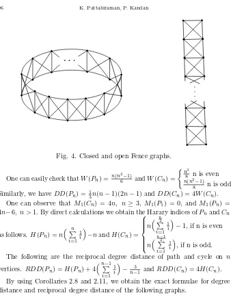
r2_RDD₍_G_{) + 2}_r₍_r₋₁₎_H₍_G_{) + 2}_r₍_r₋₁₎_m₊_n₍_r₋₁₎2_. As an application we present formulae for degree distance and reciprocal degree distance of open and closed fences,Pn⊠K2andCn⊠K2,see Fig.4.

(10)

b b b b b b b b b b b b b b b b b b b b b b

b b b

b b b b b b b b b b b b b b b b b b b b b b b

Fig. 4. Closed and open Fence graphs.

One can easily check thatW(Pn) = n(n

2

−1)

6 andW(Cn) =

(_n3

8 n is even

n(n2−1)

8 n is odd. Similarly, we haveDD(Pn) = 1₃n(n−1)(2n−1) andDD(Cn) = 4W(Cn).

One can observe that M1(Cn) = 4n, n≥ 3, M1(P1) = 0, and M1(Pn) =

4n−6, n >1.By direct calculations we obtain the Harary indices ofPnandCn

as follows. H(Pn) =n

n P i=1 1 i

−nandH(Cn) =          n n 2 P i=1 1 i

−1,if n is even

n n−1

2 P i=1 1 i

,if n is odd.

The following are the reciprocal degree distance of path and cycle on n

vertices. RDD(Pn) =H(Pn) + 4 n−1

P i=1 1 i − 3

n−1 andRDD(Cn) = 4H(Cn). By using Corollaries 2.8 and 2.11, we obtain the exact formulae for degree distance and reciprocal degree distance of the following graphs.

Example _2.12. ₍_i₎_DD₍_P_n_⊠_K₂_{) =}4 3

5n3₋₆_n2_{+ 31}_n₋₂₄_. (ii)DD(Cn⊠K2) =

(

5n(n2_{+ 2) n is even} 5n(n2_{+ 1) n is odd}_. (iii)RDD(Pn⊠K2) = 16

n P i=1 1 i + 32

n−1

P

i=1 1

i

−6n−_n24₋₁ −8.

(iv)RDD(Cn⊠K2) =

        

10n1 + 4

n 2 P i=1 1 i

−40 n is even

10n1 + 4

n−1 2 P i=1 1 i

n is odd.

(11)

Acknowledgments

The authors wish to thank the refrees for their recommendations to publish this article.

References

1. Y. Alizadeh, A. Iranmanesh, T. Doslic, Additively Weighted Harary Index of Some Com-posite Graphs,Discrete Math.,313_{, (2013), 26-34.}

2. S. Chen , W. Liu , Extremal Modified Schultz Index of Bicyclic Graphs,MATCH Com-mun. Math. Comput. Chem.,64_{, (2010), 767-782.}

3. J. Devillers, A. T. Balaban,Topological Indices and Related Descriptors in QSAR and QSPR, Gordon and Breach, Amsterdam, The Netherlands, 1999.

4. A. A. Dobrynin, A. A. Kochetova, Degree Distance of a Graph: a Degree Analogue of the Wiener Index,J. Chem. Inf. Comput. Sci.,34, (1994), 1082-1086.

5. T. Doslic, A. Graovac, F. Cataldo, O. Ori, Notes on Some Distance-Based Invariants for 2-Dimensional Square and Comb Lattices,Iranian Journal of Mathematical Sciences and Informatics,2_{(5), (2010), 61-68.}

6. B. Furtula, I. Gutman, Z. Tomovic, A. Vesel, I. Pesek, Wiener-Type Topological Indices of Phenylenes,Indian J. Chem.,41A_{, (2002), 1767-1772.}

7. I. Gutman, Selected Properties of the Schultz Molecular Topological Index, J. Chem. Inf. Comput. Sci.,34_{, (1994), 1087-1089.}

8. I. Gutman, O.E. Polansky, Mathematical Concepts in Organic Chemistry, Springer-Verlag, Berlin, 1986.

9. I. Gutman, A Property of the Wiener Number and Its Modifications,Indian J. Chem., 36A, (1997), 128-132.

10. I. Gutman, A. A. Dobrynin, S. Klavzar. L. Pavlovic, Wiener-Type Invariants of Trees and Their Relation,Bull. Inst. Combin. Appl.,40, (2004), 23-30.

11. I. Gutman, D. Vidovic, L. Popovic, Graph Representation of Organic Molecules. Cayley’s Plerograms vs. His Kenograms,J.Chem. Soc. Faraday Trans.,94, (1998), 857-860. 12. A. Hamzeh, A. Iranmanesh, S. Hossein-Zadeh , M.V. Diudea, Generalized Degree

Dis-tance of Trees, Unicyclic and Bicyclic Graphs, Studia Ubb Chemia., LVII,4_{, (2012),} 73-85.

13. A. Hamzeh, A. Iranmanesh, S. Hossein-Zadeh, Some Results on Generalized Degree Distance,Open J. Discrete Math.,3, (2013), 143-150.

14. B. Horoldagva , I. Gutman , On Some Vertex-Degree-based Graph Invariants,MATCH Commun. Math Comput. Chem.,65, (2011), 723-730.

15. H. Hua, S. Zhang, On the Reciprocal Degree Distance of Graphs,Discrete Appl. Math., 160, (2012), 1152-1163.

16. O. Ivanciuc, T. S. Balaban, Reciprocal Distance Matrix Related Local Vertex Invariants and Topological Indices,J. Math. Chem.,12_{, (1993), 309-318.}

17. A. Iranmanesh, Y. Aliazdeh, Computing Wiener Index ofHAC5C7[p, q] Nanotubes by Gap program,Iranian Journal of Mathematical Sciences and Informatics,1_{(3), (2008),} 1-12.

18. O. Khormali , A. Iranmanesh , I. Gutman , A. Ahamedi , Generalized Schultz Index and Its Edge Versions,MATCH Commun. Math Comput. Chem.,64, (2010), 783-798. 19. S. C. Li, X. Meng, Four Edge-Grafting Theorems on the Reciprocal Degree Distance

of Graphs and Their Applications,J. Comb. Optim., (2013), DOI 10.1007/s 10878-013-9649-1.

20. A. Mamut, E. Vumar, Vertex Vulnerability Parameters of Kronecker Products of Com-plete Graphs,Inform. Process. Lett.,106, (2008), 258-262.

(12)

21. K. Pattabiraman, M. Vijayaragavan, Reciprocal Degree Distance of Some Graph Oper-ations,Transactions on Combinatorics,2, (2013), 13-24.

22. K. Pattabiraman, M. Vijayaragavan, Reciprocal Degree Distance of Product Graphs, Discrete Appl. Math.,179, (2014), 201-213.

23. G. F. Su, L.M. Xiong, X.F. Su, X.L. Chen, Some Results on the Reciprocal Sum-Degree Distance of Graphs,J. Comb. Optim., (2013) DOI 10.1007/s 10878-013-9645-5. 24. I. Tomescu, Some Extremal Properties of the Degree Distance of a Graph,Discrete Appl

Math,98, (1999), 159-163.

25. I. Tomescu, Properties of Connected Graphs Having Minimum Degree Distance,Discrete Math,309, (2008), 2745-2748.

26. H. Wang, L. Kang, Further Properties on the Degree Distance of Graphs, J. Comb Optim., DOI 10.1007/s10878-014-9757-6.

27. H. Y. Zhu, D.J. Klenin, I. Lukovits, Extensions of the Wiener Number,J. Chem. Inf. Comput. Sci.,36_{, (1996), 420-428.}