Influences of magnetic field in viscoelastic fluid

ISSN: 2008-6822 (electronic)

http://dx.doi.org/10.22075/ijnaa.2017.1451.1367

Influences of magnetic field in viscoelastic fluid

Kashif Ali Abroa,∗, Mirza Mahmood Baigb, Mukarrum Hussainc

a_{Department of Basic Sciences and Related Studies, Mehran University of Engineering and Technology, Jamshoro, Pakistan} b_{Department of Mathematics, NED University of Engineering Technology, Karachi, Pakistan}

c_{Institute of Space Technology, Karachi, Pakistan}

(Communicated by M. Eshaghi)

Abstract

This communication influences on magnetohydrodynamic flow of viscoelastic fluid with magnetic field induced by oscillating plate. General solutions have been found out for velocity and shear stress profiles using mathematical transformations (integral transforms). The governing partial differential equations have been solved analytically under boundary conditions u(0, t) = A0H(t)sin(Ωt) and u(0, t) = A0H(t)cos(Ωt) with t ≥ 0. For the sake of simplicity of boundary conditions are verified

on the analytical general solutions and similar solutions have been particularized under three limited cases namely (i) Maxwell fluid without magnetic field if γ 6= 0, M = 0 (ii) Newtonian fluid with magnetic field if γ = 0, M 6= 0 and (iii) Newtonian fluid with out magnetic field if γ = 0, M = 0. Finally various physical parameters with variations of fluid behaviors are analyzed and depicted graphical illustrations.

Keywords: MHD Maxwell fluid, Laplace and Fourier transforms, rheological Parameters.

2010 MSC: Primary 26A25; Secondary 39B62.

Nomenclature: M Magnetic parameter,A0 Non-zero constant, γ Relaxation time, H(t) Heaviside

function, Q Cauchy stress tensor, N Extra-stress tensor,B Rivlin Ericksen tensor, −pI Spherical stress, Ω Frequency, ν Kinematic viscosity, µ dynamic Viscosity, ρ Density, t Time, T Transpose,

η Fourier sine transform parameter, δ Laplace transform parameter, u(y, t) Velocity Field, τ(y, t) Shear Stress.

∗_{Corresponding author}

Email addresses: kashif.abro@faculty.muet.edu.pk(Kashif Ali Abro), baig@neduet.edu.pk(Mirza Mahmood Baig),mrmukkarum@yahoo.com(Mukarrum Hussain)

1. Introduction

The analysis of non-Newtonian fluid flows in magnetohydrodynamics (MHD) has diverted attention of mathematician, engineers and researchers. Because such phenomenon usually arises among various fields for instance, nuclear fuel debris treatment, the geothermal sources investigation, metal alloys, optimization of solidification processes of metals and many others. Newtonian fluids are subtle in contrast with non-Newtonian fluids. Due to this fact, most of resultant governing equations arise from non-Newtonian fluid when magnetohydrodynamics (MHD) flow is considered, these equations becomes very complex to solve due to their appearance of nonlinearity. Magnetohydrodynamic non-Newtonian fluid flows have been studies with various aspects which can be found in recent references [3], [10], [11], [12], [13]. Due to several applications in engineering and science, flow of electrically conducting (magnetohydrodynamics) viscoelastic fluids has diverted the interest of researchers. In geophysics, magnetohydrodynamics is applicable to study and measure the velocities and positions of frame of reference on the earth’s surface that gets rotations towards the frame of inertial along with magnetic field. In the geophysical and astrophysical dynamics, magnetohydrodynamics is used for the analysis of inter planetary and inter stellar matter, solar storms and flares, stellar and solar structure and several others. MHD in engineering point of view finds its usefulness in industrial equipment such as MHD boundary layer control of reentry vehicles, MHD generators, MHD pumps, magnetic drug targeting, MHD bearings, ion propulsion and many others. Keeping the above motivations in mind, many researchers are busy for sharing valuable contributions regarding magnetohydrodynamics [1], [2], [4], [5], [6], [7], [8], [9], [14], [15], [16]. However, this article explores the influences on magnetohydrodynamic flow of viscoelastic fluid with and without magnetic field induced by oscillating plate. General solutions have been found out for velocity and shear stress profiles using mathematical transformations (Integral transforms). The governing partial differential equations have been solved analytically under boundary conditions u(0, t) = A0H(t)sin(Ωt) and u(0, t) = A0H(t)cos(Ωt) with t≥0. For the sake of simplicity of boundary conditions are verified on the analytical general solutions and similar solutions have been particularized under three limited cases namely (i) Maxwell fluid with out magnetic field ifγ 6= 0, M = 0 (ii) Newtonian fluid with magnetic field if γ = 0, M 6= 0 and (iii) Newtonian fluid with out magnetic field if γ = 0, M = 0. Finally various physical parameters with variations of fluid behaviors are analyzed and depicted graphical illustrations.

2. Formulation of Flow Equations

The electrically conducting flows of an incompressible fluid due to body forces are

∇.W = 0,∇.Q={Wt+ (W.∇)W}ρ+σM02W, (2.1)

where, W is the velocity field, ∇ represents the dell operator, Q is Cauchy stress, ρ is density of fluid, M0 is the applied magnetic field and t is the time. The assumption of Reynolds number for

small magnetic field is induced uniformly. The Cauchy stress Q in an incompressible Maxwell fluid is given by

Q=−pI+N,N+λ( ˙N−PN−NPT) =µB, (2.2)

where, Q is Cauchy stress,−pI denotes the indeterminate spherical stress, N is extra-stress tensor,

γ is relaxation time, P is the velocity gradient, B=P+PT is the first Rivlin Ericksen tensor, µis the dynamic viscosity of the fluid, the superscript T indicates the transpose operation. Velocity is assumed as Wand having an extra-stress tensor N

If we consider the fluid is at rest up to the moment t= 0, then

W= (y,0) = 0,N= (y,0) = 0, (2.4)

and equations (2.2), (2.3) and (2.4) imply Nyz =Nyy =Nxz =Nzz = 0,

γ ∂ ∂t+ 1

τ(y, t)−µ∂u(y, t)

∂t = 0. (2.5)

Without body forces, the balance of linear momentum lessens to

∂p

∂x +σM 2

0u(y, t)−

∂τ(y, t)

∂t +ρ

∂u(y, t)

∂t = 0, σM 2

0u(y, t) =− ∂p ∂y, σM

2

0u(y, t) =− ∂p

∂z. (2.6)

Eliminating τ between equations(2.5) and (2.6), then the equation are

γ ∂ ∂t+ 1

∂u(y, t)

∂t =−

γ ∂ ∂t + 1

1

ρ ∂p ∂x +ν

∂2u(y, t)

∂t2 − σM₀2

ρ

γ ∂ ∂t + 1

u(y, t);y, t >0. (2.7)

The governing equations corresponding to an incompressible MHD Maxwell fluid are

γ ∂ ∂t+ 1

∂u(y, t)

∂y +ν

∂2u(y, t)

∂t2 +M

γ ∂ ∂t+ 1

u(y, t) = 0, (2.8)

γ ∂ ∂t+ 1

τ(y, t) =µ∂u(y, t)

∂y , (2.9)

where M = σM02 ρ .

3. Initial and Boundary Conditions of the Probelem

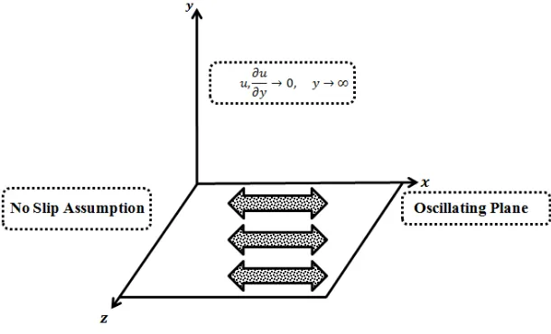
Let incompressible MHD Maxwell fluid possessing the space lying over an infinitely oscillating plane which is positioned in the xz plane and perpendicular to the y-axis. Initially, the fluid is at rest and at the moment t = 0+ _{the plane is impulsively brought to velocity u(0, t) = A}

0H(t)sin(Ωt) or u(0, t) = A0H(t)cos(Ωt) in its own plane. Due to the shear, the fluid above the plane is gradually

moved. Its velocity is of the form (2.4) and appropriate initial and boundary conditions are as sketched in Fig. 1.

u(y,0) = ∂u(y,0)

∂t = 0, τ(y,0) = 0, y >0, (3.1)

u(0, t) = A0H(t)sin(Ωt), u(0, t) = A0H(t)cos(Ωt), t≥0, (3.2)

naturally

u(y, t),∂u(y, t)

∂t →0, as y→ ∞ and t >0, (3.3)

Figure 1: Geometry of the problem under the oscillations of a plate.

4. Solution of Sine Oscillations

4.1. Velocity Field

Employing Fourier sine transform on (2.8) and taking conditions (3.1), (3.2), (3.3). We have

∂us(η, t) ∂t +γ

∂2_u s(η, t)

∂t2 =−νη 2_u

s(η, t) +νη

r

2

πA0H(t)cos(Ωt)−M

γ ∂ ∂t + 1

us(η, t), (4.1)

whereus(η, t) is Fourier sine transform, H(t) is the Heaviside function and Fourier sine transform is

defined by

us(η, t) =

r

2

π

Z ∞

0

sin(yη)u(y, t)dy. (4.2)

The following initial conditions are satisfied by Fourier sine transform,

us(η,0) =

∂us(η,0)

∂t = 0, η >0. (4.3)

Applying the Laplace transform to (4.1), we find that

¯

us(η, δ) =

r

2

π

A0 ν η Ω

(δ2_{+ Ω}2_)[γδ2_{+ (1 +γM)δ+M +νη}2_], (4.4)

breaking (4.4) in below expression as in equivalent form

¯

us(η, δ) =

A0 ν η Ω

(M +νη2₎

r

2

π

1

(δ2_{+ Ω}2₎ −

δ(1 +γδ+M γ)

(δ2_{+ Ω}2_)[γδ2_{+ (1 +γM)δ+M +νη}2_]

. (4.5)

Inverting (4.5) by Fourier sine transformation, we can write ¯us(η, δ)

¯

u(y, δ) (4.6)

= 2A0νηΩ_π

q

2 π

R∞

0

ηsin(yη) (M+νη2₎

1 (δ2_+Ω2₎ −

δ(1+γδ+M γ)

(δ2_+Ω2_)[γδ2_{+(1+γM)δ+M+νη}2_]

Finally we apply the inverse Laplace transform and its convolution theorem to (4.6), having the below fact

Z ∞

0

ηsin(yη) (q2_+η2₎ =

2

πe

−qy_{, q >0. (4.8)}

Velocity field is expressed in multiple integral form as,

u(y, t) =A0H(t)sin(Ωt)e− √

M

νy− 2A0H(t)Ων

πγ(δ1−δ2)

Z ∞

0

Z t

0

ηsin(yη)

(M+νη2₎cosΩ(t−z)

×

(1 +γδ1)eδ1z−(1 +γδ2)eδ2z

dη dz+ 2A0H(t)ΩνM

π(δ1−δ2)

Z ∞

0

Z t

0

ηsin(yη) (M +νη2₎

×cosΩ(t−z)(eδ1t−eδ2t) dη dz, (4.9)

where,δ1, δ2 =

−(1+γM)±√(1+γM)2_{−4γ(M+νη}2₎

2γ are the roots of the algebraic equation γδ2_{+ (1 +γM)δ+ (M +νη}2_{) = 0.}

4.2. Shear Stress

Applying Laplace transform to equation (2.9) the expression takes place as,

¯

τ(y, δ) = µ (1 +γδ)

∂u¯(y, δ)

∂y . (4.10)

Solving (4.6) for partial differentiation, with respect to y, we get

∂u¯(y, δ)

∂y

= 2A0νΩ

π

Z ∞

0

η2cos(yη) (M +νη2₎

1 (δ2_{+ Ω}2₎−

δ(1 +γδ+M γ)

(δ2_{+ Ω}2_)[γδ2_{+ (1 +γM)δ+M +νη}2_]

dη.

(4.11)

Substituting equation (4.11) in (4.10), we have

¯

τ(y, δ) = µ (1 +γδ)

×

2A0νΩ

π r 2 π Z ∞ 0

η2cos(yη) (M+νη2₎

1 (δ2_{+ Ω}2₎−

δ(1 +γδ+M γ)

(δ2_{+ Ω}2_)[γδ2_{+ (1 +γM)δ+M+νη}2_]

dη.

(4.12)

Simplifying (4.12) for suitable expression of shear stress as

¯

τ(y, δ) =− µ

(1 +γδ)

r

M ν

A0Ω

(δ2_{+ Ω}2₎e −√M

νy− 2A0νΩµ

π

Z ∞

0

η2cos(yη) (M +νη2₎

δ

(δ2_{+ Ω}2₎

×

1

δ−δ1

− 1

δ−δ2

dη+2M A0µΩν

π(δ1−δ2)

Z ∞

0

η2cos(yη) (M +νη2₎

δ

(δ2_{+ Ω}2₎

×

1

(δ−δ1)(1 +δ1γ)

− 1

(δ−δ2)(1 +δ2γ)

+ γ

2_(δ

1−δ2)

(1 +δ1γ)(1 +δ2γ)(1 +δγ)

Finally, applying inverse Laplace transform on equation (4.13), we get shear stress in integral form

τ(y, t) =−A0H(t)µ

γ

r

M ν e

−√M νy

Z t

0

sinΩ(t−z)ezγdz −2A0H(t)νΩµ

πγ(δ1−δ2)

Z ∞

0

η2cos(yη) (M +νη2₎

×cosΩ(t−z)(eδ1z−eδ2z) dη dz+2M A0H(t)µΩν

π(δ1−δ2)

Z ∞

0

η2cos(yη)

(M+νη2₎cosΩ(t−z)

×

eδ1z

(1 +δ1γ)

− e

δ2z

(1 +δ2γ)

+ γ

2_(δ

1−δ2)e −z

γ

(1 +δ1γ)(1 +δ2γ)

dη dz. (4.14)

Solution for cosine oscillations: Solution of cosine oscillation is obtained by utilization of similar algorithm

u(y, t) =A0H(t)cos(Ωt)e− √

M

νy − 2A0H(t)Ων

πγ(δ1−δ2)

Z ∞

0

Z t

0

ηsin(yη)

(M +νη2₎sinΩ(t−z)

×

(1 +γδ1)eδ1z−(1 +γδ2)eδ2z

dη dz+ 2A0H(t)ΩνM

π(δ1−δ2)

Z ∞

0

Z t

0

ηsin(yη) (M +νη2₎

×sinΩ(t−z)(eδ1z−eδ2z) dη dz, (4.15)

τ(y, t) =−A0H(t)µ

γ

r

M ν e

−√M νy

Z t

0

cosΩ(t−z)ezγ_dz− 2A0H(t)νΩµ

π

Z ∞

0

ηcos(yη) (M+νη2₎

×sinΩ(t−z)

eδ1z−eδ2z

dη dz+2M A0H(t)µΩν

π(δ1−δ2)

Z ∞

0

η2_cos(yη)

(M +νη2₎sinΩ(t−z)

×

eδ1z

(1 +δ1γ)

− e

δ2z

(1 +δ2γ)

+ γ

2_(δ

1−δ2)e −z

γ

(1 +δ1γ)(1 +δ2γ)

dη dz. (4.16)

5. Particular Cases

5.1. Solutions of Maxwell Fluid M = 0 (Absence of Magnetic Field)

Solutions of Maxwell fluid are obtained when limit M → 0 into equations (4.9), (4.14), (4.15) and (4.16)

uM S(y, t) =A0H(t)sin(Ωt)−

2A0H(t)Ων π(δ1−δ2)

Z ∞

0

Z t

0

sin(yη)

η cosΩ(t−z)

×[(1 +γδ1)eδ1z−(1 +γδ2)eδ2z] dη dz, (5.1)

τM S(y, t) = −

2A0H(t)νΩ π(δ1−δ2)

Z ∞

0

Z t

0

cos(yη)cosΩ(t−z)[eδ1z−eδ2z]dη dz, (5.2)

uM C(y, t) =A0H(t)cos(Ωt)−

2A0H(t)Ων π(δ1−δ2)

Z ∞

0

Z t

0

sin(yη)

η sinΩ(t−z)

×[(1 +γδ1)eδ1z−(1 +γδ2)eδ2z] dη dz, (5.3)

τM C(y, t) =−

2A0H(t)νΩ π

Z ∞

0

Z t

0

cos(yη)

η sinΩ(t−z)[e

5.2. MHD Newtonian Fluid γ = 0 (Presence of Magnetic Field)

Solutions of MHD Newtonian fluid are obtained when limit γ = 0 into equations (4.9),(4.14),(4.15) and (4.16) along with usage of following facts

limγ→0δ1 =−(M +νη2), limγ→0δ2 =∞, limγ→0γ(δ1−δ2) = 1

uM N S(y, t)

=A0H(t)sin(Ωt)e− √

M

νy − 2A0H(t)Ων

π

Z ∞

0

Z t

0

ηsin(yη)

(M +νη2₎cosΩ(t−z)e

−(M+νη2_)z

dη dz,

τM N S(y, t) =−µA0H(t)

r

M

ν sin(Ωt)e

−√M

νy − 2A0H(t)νΩµ

π

Z ∞

0

Z t

0

η2_cos(yη)

(M+νη2₎

×cosΩ(t−z)e−(M+νη2)z dη dz,

uM N C(y, t)

=A0H(t)cos(Ωt)e− √

M

νy− 2A0H(t)Ων

π

Z ∞

0

Z t

0

ηsin(yη)

(M+νη2₎sinΩ(t−z)e

−(M+νη2_)z

dη dz,

τM N C(y, t) =

2A0H(t)νΩµ π

Z ∞

0

Z t

0

ηcos(yη)

(M +νη2₎sinΩ(t−z)e

−(M+νη2_)z

dη dz.

5.3. Newtonian Fluid γ = 0 and M = 0 (Absence of Magnetic Field)

Solutions of Newtonian fluid are obtained when limit γ = 0 and M = 0 into equations (4.9), (4.14), (4.15) and (4.16)

uN S(y, t) = A0H(t)sin(Ωt)−

2A0H(t)Ω π

Z ∞

0

Z t

0

sin(yη)

η cosΩ(t−z)e

−νη2z _{dη dz,}

τN S(y, t) =−

2A0H(t)νΩµ π

Z ∞

0

Z t

0

cos(yη)cosΩ(t−z)e−νη2z dη dz,

uN C(y, t) =A0H(t)cos(Ωt)−

2A0H(t)Ω π

Z ∞

0

Z t

0

sin(yη)

η sinΩ(t−z)e

−νη2_z

dη dz,

τN C(y, t) = −

2A0H(t)Ωµ π

Z ∞

0

Z t

0

cos(yη)cosΩ(t−z)e−νη2z dη dz.

6. Conclusion

In this portion, the characteristics of magnetohydrodynamic flow of viscoelastic fluid with and with-out magnetic field induced by oscillating plate are shown. General solutions have been found with-out for velocity and shear stress profiles using mathematical transformations (Integral transforms) under the sine and cosine boundary conditions u(0, t) = A0H(t)sin(Ωt) and u(0, t) =A0H(t)cos(Ωt) with t ≥0. For the sake of simplicity of boundary conditions are verified on the analytical general solu-tions and similar solusolu-tions have been particularized under three limited cases namely (i). Maxwell fluid with out magnetic field if γ 6= 0 and M = 0 (ii). Newtonian fluid with magnetic field if γ = 0 and M 6= 0 and (iii). Newtonian fluid with out magnetic field if γ = 0 and M = 0. The bunch of graphs has been prepared with typical values at different situations for rheological parameters to reveal some relevant physical aspects. Finally various outcomes are discussed below:

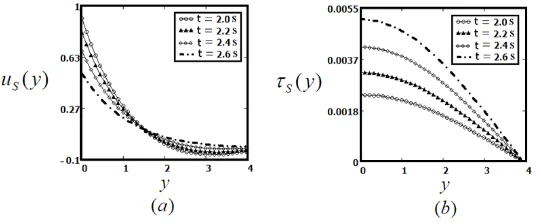
The influence on fluid motion is displayed in Fig. 2 for the sine and cosine oscillations. It is noticed that by increasing various values of time t = 2.0,2.2,2.4,2.6 the velocity of fluid is increasing on the entire boundary region which indicates that as time progresses fluid velocity is monotonically enhanced.

Fig. 3 represents the relaxationγ phenomenon of fluid between 1≤γ ≤4, both velocity field as well as shear stress have strong effects on decreasing fluid behavior as expected.

The viscous effects ν are shown in Fig. 4 in which velocity field is thickening and shear stress is scattering when viscosity? increases, such phenomenon is termed as shear thinning and shear thickening.

Impacts of magnetic field M on fluid motion are displayed in Fig. 5 in which velocity field and shear stress decreases when magnetic parameter increases. As we expected in MHD flow, wall regions will be balanced if fluid velocity decreases.

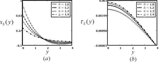
Fig. 6 is prepared to analyze the impact of oscillations, It is noted that increase in fluid oscillations Ω approaches to zero and decays away from the oscillating plate. Meanwhile, Fig. 7 show the behavior of plate in terms of helical oscillations.

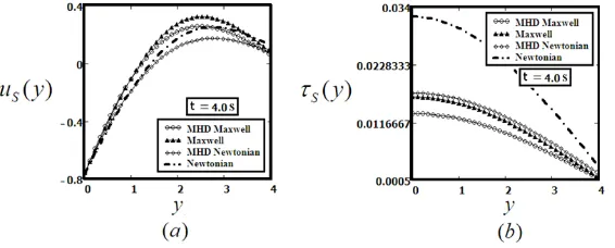
Figs. 8 and 9 are depicted for comparison of four kinds of models i-e Maxwell fluid in presence of magnetic field, Maxwell fluid in absence of magnetic field, Newtonian fluid in presence of magnetic field and Newtonian fluid in absence of magnetic field, the motion of fluid flow is contrasting, i-e velocity field is increasing and shear stress is scattering with respect to different increasing effects of time parameter t.

Figure 3: Profiles of the velocity field u(y, t) and the shear stress τ(y, t) for MHD Maxwell fluid given by equations (4.8) and (4.13), forA0= 1, ν= 0.63, µ= 1.52, t= 2s, M = 0.5, Ω = 1 and different values ofγ.

Figure 4: Profiles of the velocity field u(y, t) and the shear stress τ(y, t) for MHD Maxwell fluid given by equations (4.8) and (4.13), forA0= 1, ρ= 2.41, µ= 1.52, γ= 2, M= 0.5, Ω = 1 and different values ofν.

Figure 5: Profiles of the velocity field u(y, t) and the shear stress τ(y, t) for MHD Maxwell fluid given by equations (4.8) and (4.13), forA0= 1, ν= 0.63, µ= 1.52, γ= 2, t= 2s, Ω = 1 and different values ofν.

Figure 7: Profiles of the velocity field u(y, t) and the shear stress τ(y, t) for MHD Maxwell fluid given by equations (4.8) and (4.13), forA0= 1, ν= 0.63, µ= 1.52, γ= 2, M = 0.5,Ω = 1, and different values ofy.

Figure 8: Profiles of the velocity fieldu(y, t) and the shear stressτ(y, t) for MHD Maxwell fluid, Maxwell fluid, MHD Newtonian fluid and Newtonian fluid given by equations (4.8), (4.13), (5.1), (5.2), (5.5), (5.6), (5.9) and (5.10) for

A0= 1, ν= 0.63, µ= 1.52, γ= 2, M = 0.5,Ω = 1, and fixed value fort= 2.5s.

Figure 9: Profiles of the velocity fieldu(y, t) and the shear stressτ(y, t) for MHD Maxwell fluid, Maxwell fluid, MHD Newtonian fluid and Newtonian fluid given by equations (4.8), (4.13), (5.1), (5.2), (5.5), (5.6), (5.9) and (5.10) for

A0= 1, ν= 0.63, µ= 1.52, γ= 2, M = 0.5,Ω = 1, and fixed value fort= 4.0s.

Acknowledgments

The author Kashif Ali Abro is highly thankful and grateful to the Mehran University of Engineering and Technology, Jamshoro, Pakistan for facilitating this research work.

References

[1] K.A. Abro,Porous effects on second grade fluid in oscillating plate, J. Appl. Environ. Biol. Sci., 6 (2016) 71–82. [2] A. Borrelli, G. Giantesio and M.C. Patria,An exact solution for the 3D MHD stagnation-point flow of a micropolar

fluid, Commun. Nonlinear Sci. Numer. Simul., 20 (2015) 121–135.

[4] M. Jamil, K.A. Abro and N.A. Khan, Helices of fractionalized Maxwell fluid, Nonlinear Engineering., 4 (2015) 191–201.

[5] M. Khan, M. Arshad and A. Anjum, On exact solutions of Stokes second problem for MHD Oldroyd-B fluid, Nucl. Eng. Des., 243 (2012) 20–32.

[6] N.A. Khan, A. Mahmood, M. Jamil and N.U. Khan,Traveling wave solutions for MHD aligned flow of a second grade fluid, Int. J. Chm. React. Engg., 8 (2010) A163.

[7] K.A. Abro, M. Hussain and M.M. Baig,Impacts of Magnetic Field on Fractionalized Viscoelastic Fluid, J. Appl. Environment. Bio. Sci., 6 (2016) 84–93.

[8] Y. Liu, L. Zheng and X. Zhang, Unsteady MHD Couette flow of a generalized Oldroyd-B fluid with fractional derivative, Comput. Math. Appl.-A., 61 (2011) 443–450.

[9] Y. Liu, L. Zheng, X. Zhang and F. Zong,The oscillating flows and heat hransfer of a generalized Oldroyd-B fluid in magnetic field, IAENG Int. J. Appl. Math., 40 (2010) 04–08.

[10] A. Mehmood, A. Ali and T. Mahmood,Unsteady magnetohydrodynamic oscillatory flow and heat transfer analysis of a viscous fluid in a porous channel filled with a saturated porous medium, J. Porous Media., 13 (2010) 573–577. [11] S. Nadeem, Rizwan Ul Haq, N.S. Akbar and Z.H. Khan,MHD three-dimensional Casson fluid flow past a porous

linearly stretching sheet, Alexandria Eng. J., 52 (2013) 577–582.

[12] T.M. Nabil, G.M. Moatimid and S.M. Hoda, Magnetohydrodynamic flow of non-Newtonian visco-elastic fluid through a porous medium near an accelerated plate, Can. J. Phys., 81 (2003) 1249–1269.

[13] T.M. Nldabe and S.N. Sallam,Non-Darcy couette flow through a porous medium of magnetohydrodynamic visco-elastic fluid with heat and mass transfer, Can. J. Phys., 83 (2005) 1241–1263.

[14] K.D. Singh, Exact solution of MHD mixed convection periodic flow in a rotating vertical channel with heat radiation, Int. J. of App. Mech. and Engg., 18 (2013) 853–869.

[15] H. Zaman, Z. Ahmad and M. Ayub,A note on the unsteady incompressible MHD fluid flow with slip conditions and porous walls, ISRN Mathematical Physics.Volume 2013, Article ID 705296.