Volume 6 | Issue 1
Article 9
Single Image Super-Resolution
Yujing Song
University of Minnesota - Morris
Follow this and additional works at:
https://digitalcommons.morris.umn.edu/horizons
Part of the
Graphics and Human Computer Interfaces Commons
This Article is brought to you for free and open access by the Journals at University of Minnesota Morris Digital Well. It has been accepted for inclusion in Scholarly Horizons: University of Minnesota, Morris Undergraduate Journal by an authorized editor of University of Minnesota Morris Digital Well. For more information, please [email protected].
Recommended Citation
Song, Yujing () "Single Image Super-Resolution,"Scholarly Horizons: University of Minnesota, Morris Undergraduate Journal: Vol. 6 : Iss. 1 , Article 9.
Single Image Super-Resolution
Yujing Song
Division of Science and Mathematics University of Minnesota, Morris Morris, Minnesota, USA 56267
[email protected]
ABSTRACT
Super-Resolution (SR) of a single image is a classic problem in computer vision. The goal of image super-resolution is to produce a high-resolution image from a low-resolution im-age. This paper presents a popular model, super-resolution convolutional neural network (SRCNN), to solve this prob-lem. This paper also examines an improvement to SRCNN using a methodology known as generative adversarial net-work (GAN) which is better at adding texture details to the high resolution output.
1.
INTRODUCTION
Image super-resolution is a concept based on the human visual system. David Hubel, Torsten Wisel, the winners of 1981 Nobel Prize in medicine, found that information pro-cessing in the human visual system is hierarchical [8]. Us-ing convolutional neural networks to deal with SR problems mimics the processing of the human visual system. There-fore, computer vision is a good applications of neural net-works. Super-resolution is a classic application of computer vision, and tends to produce images that people find either realistic or aesthetically pleasing.
This paper looks into the working processes of super-resolution using convolutional neural networks (SRCNN) and the improvements that result from a modification to the process using a generative adversarial network known as SR-GAN. Section 2 gives the background knowledges. Section 3 introduces each step for establishing a SRCNN model. Sec-tion 4 discusses, SRGAN, a recent popular method, that has some improvement over SRCNN. Section 5 explains the relationship between SRCNN and SRGAN.
2.
BACKGROUND
In this section, we introduce some significant concepts re-lated to understanding the use of convolutional neural works for image problems, including classical neural net-works, convolutional neural netnet-works, and loss functions. We also discuss recognizing images’ construction.
2.1
Images
Two concepts are important for understanding an image, one is channels, the other is pixels.
This work is licensed under the Creative Commons Attribution-NonCommercial-ShareAlike 4.0 International License. To view a copy of this license, visit http://creativecommons.org/licenses/by-nc-sa/4.0/. UMM CSci Senior Seminar Conference, November 2018Morris, MN.
A color image usually is an RGB image, which means it is composed of red, green and blue components. If an image is split into its components, then we have three channels, one for each color. There are other ways, than RGB, to store color information for an image. Another common approach is YCbCr– which also uses 3 channels, but in this encoding Y represents luminance (brightness) while Cb and Cr are a more complicated way to represent colors (see [1] for details). Pixels are the smallest unit of a digital image. For the images used by SRCNN and SRGAN these pixel values are numbers from 0 to 255. If we have an image with sizew×l, this means that the image is divided evenly intowrows of pixels, and each row haslpixels. Each channel has its own pixel value in every pixel position. Every pixel position in a channel corresponds to the same positions in the other channels. When these pixel values are put together, a spe-cific color shows up in spespe-cific position in the image. In short, a pixel is a location in an image in an RGB image it takes 3 values (one for each channel) to indicate the color associated to that pixel.
Patches of an image means a part of an image, which contains the specific size of pixel values of an image. For example, the original image will be cut into as many 33×33 patches to set as inputs in the convolutional neural network. Image upscaling is trying to express an image using more pixels. For example, if an image is expressed by 10×10 pixels in the beginning, after 2 times upscaling, it is expressed by 20×20 pixels. Since pixels are the smallest unit of an image, the size of each pixel stays the same, so the upscaled image is enlarged by the process of image upscaling. The popular two algorithms to upscale are bicubic interpolation and sparse-coding base method [1].
Bicubic interpolation is the most commonly used inter-polation method in two-dimensional space. In this method, the value of the function at a specific point can be obtained by the weighted average of the nearest 16 sampling points in the rectangular grid, where two polynomial interpolation cubic functions are needed, one in each direction [4]. Sparse-coding method is trying to represent an image as a linear combination of patches, and to require only a few patches to represent the image [9].
These two methods are also the two classical models for images super-resolution. Similarly, image down-scaling is trying to express an image using fewer pixels.
that are consistent with the image being upscaled. High-frequency means the High-frequency changes fast. The High-frequency in an image represent the difference between adjacent color blocks. Details in images can be described using terms like low-frequency or high-frequency. The first refers to proper-ties that change slowly– for example in a picture of a grassy hill and a clear blue sky, the blue pixels that are part of the sky may have similar values that don’t change quickly from pixel to pixel. However the pixels that make up the grass on the hill will have edges and shadows where the values of the pixels will change rapidly over short distances. The first type of detail I called low-frequency, and the second is called high-frequency. When an image is down-scaled, low-frequency details tend to be preserved, but high-low-frequency details are often lost, or blurred.
2.2
Classical Neural Network
Neural networks are a mathematical model that estimates the working process of human brains to recognize potential relationship within a set of data. Here in our case, the neural network is used as the most important part of a process that produces a high-resolution image from a low-resolution image.
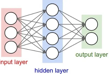
Figure 1: Basic structure of a neural network with one hid-den layer.
Figure 1 illustrates the main components of any neural network. The circles are called nodes and represent numeric values. The edges between nodes also have a numeric value called a weight. The red area on the left is the input layer, the green area on the right is the output layer, and the blue one in the middle is the hidden layer. Input layer above has 3 nodes, output layer has 2 nodes, hidden layer has 4. Note that when designing a neural network, the number of nodes are usually fixed in the input layer and output layer, but hidden layer are free. That is to say, we can set one or more hidden layers, and two or more nodes for each hidden layer. The topology and arrows in the structure of neural network diagram represent the flow of values during the calculations that transform input to output. The point of the diagram is not the nodes, but the weights. These weights need training to determine their values. Training values of the weights will be mentioned in Section 2.2.4, here we focus on understanding the structure of a neural network. We call the network fully-connected neural network because for each node in any layer, it is connected to every node in the next layer.
For every pair of adjacent layers, the nodes in a previ-ous layer,{x1, x2, ..., xn}, pass their values to the next layer
through the edges, each edge contain a weight{w}. Associ-ated to each node is both a value and a function. The value in each node, except for the values in the input layer, are produced by a calculation explained below:
y=f(b+
n
X
i=1
xi·wi)
The function associated to a node, known as the activation function, is part of the calculation that determines a nodes value. It is the functionf in the equation above. In all our neural networks, all nodes in the same layer use the same activation function. The bias b in each hidden layer is an extra weight that does not connected to any previous layer. It is added after the previous calculating process to scale a linear output up and down.
There are three types of input and output in this paper. The input will be an image and the output will be an image in the convolutional neural network (see Section 3 for details on how images are represented as the kind of numeric values that can be represented by the nodes in Figure 1). When the neural network is used in the generative network of GAN (see Section 4), the input will be a set of random numbers and the output will be an image. Whereas when the neural network is used in the discriminator network of GAN, the input will be an image and the output will be a probability (see Section 4 for details).
2.2.1
Activation function
The activation function is used to introduce the non-linearity in the neural network. Though there are a lot of activation functions, rectified linear unit (ReLU) is the only activation function we will use in this paper. The definition of ReLU is:
R(z) = max(0, z)
2.2.2
Training for neural network
Before introducing the training processes of neural net-works, we need to distinguish supervised methods and un-supervised methods. Supervised methods are “learning algo-rithms that learn to associate some input with some output, given a training set of examples of inputs and outputs” [2]. Unsupervised methods are those “that experience only ‘fea-tures’ but not a supervision signal” and try to group inputs based on their features [2]. The neural network used in CNN is a supervised method because we provide a training set for input, that are the low-resolution images, and outputs that are our original images.
image.
2.2.3
Loss function
The loss function is a method for evaluating how closely the actual output of a neural network matches the desired output. Two loss functions are used in this paper: Peak signal-to-noise ratio (PSNR) and mean square error (MSE). MSE calculates the deviation from the original values by averaging the squared difference between the estimated val-ues,Xciand the original valuesXi:
MSE = 1
n
n
X
i=1
(Xi−Xci)2
The lower the MSE value, the better the weights that have been chosen.
If we say MSE is used to judge the quality of a specific technique, PSNR is used to evaluate the quality of recon-struction of these techniques. It is an engineering term for the “ratio between the maximum possible power of a signal and the power of corrupting noise that affects the fidelity of its representation” [6]. The formula expression is the follow-ing:
PSNR = 10 log10
maxI2
MSE
where maxI is the maximum possible pixel value of the
im-age. When the pixels are represented by 8-bits per sample, its value is 255 [6]. Different with MSE, the higher value of PSNR get, the better super-resolution results a method will get.
2.2.4
Stochastic gradient descent
Since MSE evaluates the difference between the true image values and our neural networks predicted values, we want this difference as little as possible, which means we need to minimize the error. Stochastic gradient descent with back-propagation is a technique for modifying the weights in the neural network to realize this goal. These gradients will lead us to a minimum in our loss function.
In the classic neural network, the values are calculated from left to right, from input layer to output layer. But we want to minimize the mean square error by adjusting the values of weights, we need to update weights layer by layer from the output layer back to the input layer. This backward process is called back-propagation. The method that we used in back-propagation process is called stochastic gradient descent. It is called stochastic is because the sample weight value that will be updated is chosen randomly. The formula is expressed as following:
Wj+1=Wj+η·
∂L ∂Wj
where L is a loss function, and it is MSE in our case. j
represents the iteration times.Wj+1andWj are the sets of
all weights at iteration j. Wj+1is the new weight vector, it
is set to the original weight vectorWjplus the learning rate
ηtimes a partial derivative ∂W∂L j.
Learning rate, is a parameter that influences how the training occurs. The value of η controls how much ∂L
∂Wj changes the weight. The partial derivative is the fraction in the equation that displays how much the loss function will
change for every unit of original weight has changed. Note that if a weight is near its optimal value then changing the weight does not have much influence on the loss function so
∂L
∂Wj is near 0.
2.3
Convolutional Neural Network
The architecture of a neural network refers to the way in which the different layers are connected to each other. Two common ways to connect layers produce convolutional layers and fully connected layers.
2.3.1
Convolutional layer
The core of a convolutional neural network is its convolu-tional layer. To understand the details, three important con-cepts are defined: kernel, feature maps, and convolutional calculation.
Features represent some specific characteristics in an im-age. Extracting features, for example, can extract edges of an image. Kernels in convolutional network represent a fea-ture extracting method, which constrains a set of weight. A set of kernels form a filter. The number of filters in a convolutional layer is called the depth of this layer. Like each node has its own weight in neural network, each chan-nel has its own kerchan-nel in each filter. The kerchan-nel is a small array of values (in our example in Figure 2 it is 3x3). These values are treated like a sliding window and moved over the surface of the image. A sliding window is used in each chan-nels. A sliding window usually starts from the left top of the original channel, then doing convolutional calculation with its kernel. The convolutional calculation will be ex-plained in next paragraph. After the convolutions, we slide our window right-side with one pixel length. Repeat the convolutional process and slide the window again, until the end of this line. Then we move to the second row and con-tinue to do so until the window scans all the pixels in the original channels. The three sliding windows associated to a filter move across each channel at the same time and in the same fashion. At each different location a new convolutional calculation is performed.
The convolutional results are stored in the feature map. That is to say, feature map is the collection of outputs for a given filter. In our description above the sliding window was moved one pixel at a time, but often the window is moved more than one pixel– the number of pixels by which the window is moved is called the stride. In our example the stride is one, but it could be any reasonable number, it depends on the question.
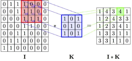
for each position. Summing up all these results, we got 4. Notice the similarity to the process of calculating the value of a node in the neural network process outlined in Section 2.2 This occurs for each position ofKas it is slid across the imageI.
Figure 2: The convolutional process example. Left is the original input channelI, the middle part is a convolutional kernelK, and right sideI∗Kis the feature map.
When calculating convolution in multi-channel input, say we have three channelsC1,C2,C3, for an RGB image, and
we know the convolutional kernels corresponding to each channel. Suppose two filters (F1andF2) and their biases (b1
andb2) are set. Let’s call the kernelsKmn, wheremstands
for the index of the filter andn stands for the index of the channel. For example,K21means it is the kernel forC1 in
F2. So the outcome will have two feature maps. The first
feature map is obtained byC1∗K11+C2∗K12+C3∗K13+b1.
The second feature map is thenC1∗K21+C2∗K22+C3∗
K23+b2, where∗represents the convolutional operation.
2.3.2
Fully connected layer
Fully connected layer acts like a generator in our case, it is trying to collect all the features in the previous layers. The fully connected layer in this case will be used in solving SR problem by CNN (details in Section 3.2), and used in the generator network of GAN (details in Section 4).
3.
SRCNN
This section discusses how convolutional neural networks are applied to the SR problem, the proposed model is called SRCNN. Given a single low-resolution image, the final high-resolution image is the output resulting from three stages of operation: patch extraction and representation (section 3.1), non-linear mapping (section 3.2), and reconstruction (section 3.3). An overview of the procedure can be seen in Figure 3.
Before we get started there is some pre-processing that must occur. To the single low-resolution image, we upscale it to the desired output resolution by first using a conven-tional technique such as bicubic interpolation. This upscaled image will be used as an input for our SRCNN. Denote the upscaled low-resolution image as input Y. We are trying to findF(Y) that is as similar as possible to the true high-resolution imageX. So F(Y) is what we obtain through SRCNN fromY,X is the original image that set as a label for adjusting weights in CNN.
3.1
Patch extraction and representation
Suppose our input image Y has size A×B, where A, B
represent the length and width respectively. Y is convolved
with kernels with sizef1×f1. The depth of this layer isn1,
that is to say,n1 filters are set in this layer. The structure
of this layer looks like what we showed in Figure 1, input layer contain the input image, then1hidden layers aren1
fil-ters, and the output layer contains the feature maps. ReLU is applied on the filter response, so we have the following equation:
F1(Y) = max(0, W1∗Y +B1),
whereW1andB1stand for the kernels in filters and the
bi-ases respectively, and∗is the convolutional operation. The value inWi, as a kernel, represents a large number of edges.
All of which share the same weights, and training occurs on this small, shared, set of weights, so it’s much more efficient to train the weights in the kernel then to train a large col-lection of independent weights. After this step, we haven1
feature maps with size (A−f1+ 1)×(B−f1+ 1), and have
removed all the negative values. [1]
The feature maps that are produced by this layer are what we mean by patch extraction and representation. The input image is the patch because it is not the original whole image but a firstly down-scaled then up-scaled sub-image, which we will introduce in Section 3.4. It is extracted byn1 kernels,
and the representations of these extractions form the feature maps.
3.2
Non-linear mapping
The second step converts then1-dimensional features into
n2 dimensions by setting n2 filters and kernels with size
f2×f2 in this layer. The operation of the second layer is:
F2(Y) = max(0, W2∗F1(Y) +B2)
W2 and B2 are the kernels and biases in the second layer,
F1(Y) is the feature maps from the last layer. Again, the
size of feature maps in F1(Y) is (A−f1+ 1)×(B−f1+
1). In order to express easily, we set A1 = (A−f1 + 1)
and B1 = (B−f1 + 1). W2 has n2 filters and B2 is n2
-dimensional. The output we get are n2 feature maps with
size (A1−f2+1)×(B1−f2+1). Similarly, we set (A1−f2+1)
asA2, (B1−f2+ 1) asB2.
Researchers inImage Super-Resolution Using Deep Con-volutional Networks [1] setf2= 1 in this layer. So we have
A2=A1, B2 =B1. It is equal to fully connected layer but
utilized 1×1 filters, which makes every position of the last layer’s feature maps share their parameters.
3.3
Reconstruction
The operation applied by the third layer produces the final high-resolution image:
F(Y) =W3∗F2(Y) +B3
W3responds to a filter that hasn3 kernels of sizef3×f3.
B3is the bias for this reconstruction layer. This layer is from
then2×1 vector produced by the previous layer. To rebuild
f3×f3image, the final high-resolution image is realized by
taking the averages of these overlapped image patches.
3.4
Training
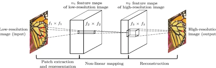
Figure 3: “Given a low resolution imageY, the first convolutional layer of the SRCNN extracts a set of feature maps. The second layer maps these feature maps non-linearly to high-resolution patch representations. The last layer combines the predictions within a spatial neighbourhood to produce the final high-resolution imageF(Y)”[1]
X are down-scaled to low-resolution samples first, and then upscaled to the target resolution using bicubic interpolation. Settings used by the researchers [1] were f1 = 9, f2 =
1, f3 = 5, n1 = 64, n2 = 32. These values were determined
by experiments and chosen to be a good balance between high-resolution quality and efficiency. MSE is used as loss functionL(Θ), Θ ={W1, W2, W3, B1, B2, B3}.:
L(Θ) = 1
n
n
X
i=1
(F(Yi; Θ)−Xi)2
wherenis the number of training samples, andXis the orig-inal image. The high-resolution imagesF(Yi; Θ) are created
by taking low-resolution imagesY as input and go through mapping functionF(Θ).
Stochastic gradient descent with back-propagation is used to minimize the loss function:
∆i+1= 0.9·∆i+η·
∂L ∂Wil
,
Wi+1l=Wil+ ∆i+1
where l ∈ {1,2,3} is the index of the channels, i is the iterations,η is the learning rate. ∆ is a parameter that its initial number is ∆0= 0.
The weights in filters are initialized by random selection. The weights will be updated by hundred of millions times via back-propagation. The learning rate is 10−4 for the first two layers but is 10−5 for the third layer.
3.5
Advantages
When the neural network is sufficiently trained, the qual-ity of the SR image is measured using the Peak Signal-To-Noise Ratio (PSNR) discussed in Section 2.2.3. The higher of PSNR, the closer the SR image is to the original. The fol-lowing table shows SRCNN is achieving better results than traditional methods in different magnifications [1]:
Eval. Mat Scale Bicubic SC SRCNN
PSNR
2 33.66 - 36.66
3 30.39 31.42 32.75
4 28.42 - 30.49
Here “Bicubic” stands for bicubic interpolation, “SC” stands for sparse-coding base method. “Scale” means the factor of
upscaling.
The table implies when upscaled two to four times of low-resolution images, SRCNN had the best PSNR values in comparison to bicubic interpolation and sparse coding base methods. That is to say, in mathematical perspective, the high-resolution images through SRCNN are closer to the original images.
4.
GAN
Study [5], uses generative adversarial network (GAN) to address the SR problem, the method is abbreviated as GAN. Based on the article, although the results of the SR-CNN process can have high PSNR values when MSE is used as the loss function, the resulting super-resolution images usually lose high-frequency details.
SRGAN is a neural network architecture composed of two competing networks, generator network and discriminator network.
The generator network creates an image by taking a set of random numbersZ. Therefore, we have two datasets in GAN, one is the true data set and the other is the fake dataset. The true data set contains original images while the fake dataset is created by the generator network.
The discriminator network is a classifier that determines if a given image is a real image from the dataset or an im-age made by generator network. Discriminator network is a binary classifier in the form of a CNN where the input is an image and the output is a probability. If the probability is greater than 0.5, the input is classified as belonging to the true dataset while a probability less than 0.5 classifies the input as belonging to the fake dataset.
The aim for the generator is to create a high-resolution image that will trick the discriminator network into classify-ing it as true. When the output of the discriminator network is close to 0.5, it means that the discriminator cannot distin-guish the difference. At this point the high-resolution image is considered to be good enough.
4.1
Training for SRGAN
processes is similar to what we have introduced in CNN (Section 2.3).
Training a generator network also requires a discriminator network. This discriminator network is put after the gener-ator network so that we can have errors to calculate the loss function. Here the labels are not important but the errors are important. The significant operation is when training the generator network, the parameters of the discriminator network should remain unchanged so that in the training process only the weights of generator network are updated. [5]
In contrast to the training process used by the generator network, which must have a discriminator network in order to calculate the error, the training discriminator network only need the discriminator network itself.
Z is a set of random numbers, andD(X) represents the probability thatXcame from the data. We train the weights ofD,WD, to maximize the probability of assigning the
cor-rect label to both training examples and samples from G. We simultaneously train the weight ofG,WG, to minimize
log(1−D(G(Z))). [3] The value function is:
min
WG max
WD
([logD(X)] + [log(1−D(G(Z)))])
The aim function above can be divided into two parts, one is for discriminator network and the other is for the generator network.
Optimizing the discriminator does not directly involve the generator network, so we only care about maximum logD(X). X is the images in the true data set, for all the images from the true dataset, the result of discriminator net-workD(X) should as close to 1 as possible. So we want to find the weights of discriminator network when the result of
D(X) is maximum.
When training the generator network, minimum log(1−
D(G(Z))) is the goal. G(Z) is equivalent to the existed fake samples. Since the samples created byG(Z) are not the real ones, we wantD(G(Z)) closer to 0.
4.2
Relationship with conventional neural
net-work
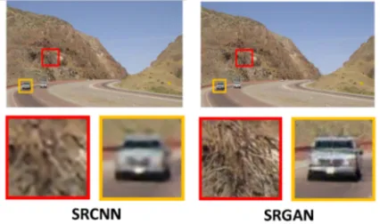
The PSNR for SRGAN is less than SRCNN, but the high-resolution image from SRGAN is visually closer to the orig-inal image, as showed in Fig.4. The car and tree in SRGAN looks more clear than that in SRCNN, though the left has PSNR 24.83db and right side SRGAN has 23.36db [7].
Figure 4: The results of high-resolution image from SRCNN and SRGAN
SRCNN used MSE as loss function, which ensured a high value for the PSNR, but a lack of high-frequency information in the image, so it over-smooths the image in a way that is obvious to people. However, SRGAN insists that the created high-resolution images should be closer to the true original images not only in the pixel values but also in the abstract characteristics. Therefore, it uses a discriminator network to judge the created images. If the discriminator network cannot distinguish if a high-resolution image is one of the true original ones, people visually cannot distinguish as well.
5.
CONCLUSION
This paper has introduced two methods to solve SR prob-lems. SRCNN is a forerunner of deep learning used in SR reconstruction. SRCNN’s network structure is very simple, using only three convolutional layers, but it improves the efficiency of the SR process and produces better PSNR than traditional methods. However, SRCNN is not perfect, it in-spired many of other methods to improve that. Every work is a great step forward but we chose SRGAN in Section 4 in this paper because it not only focus on increase the value of PSNR, but try to enhance more details in the images to improve human visual perception.
6.
REFERENCES
[1] C. Dong, K. He, C. Change Loy, and X. Tang. Image super-resolution using deep convolutional networks.
IEEE Transactions on Pattern Analysis and Machine Intelligence, 38:30–52, February 2016.
[2] I. Goodfellow, Y. Bengio, and A. Courville.Deep Learning. MIT Press., Cambridge, MA, USA, 2016. [3] I. Goodfellow, J. Pouget-Abadie, M. Mirza, B. Xu,
D. Warde-Farley, S. Ozair, A. Courville, and Y. Bengio. Generative adversarial nets.NIPS’14 Proceedings of the 27th International Conference on Neural Information Processing Systems, 2:2672–2680.
[4] R. Keys. Cubic convolution interpolation for digital image processing.IEEE Transactions on Acoustics, Speech, and Signal Processing, 29:1153 – 1160, December 1981.
[5] C. Ledig, L. Theis, F. Huszar, J. Caballero, A. Cunningham, A. Acosta, A. Aitken, A. Tejani, J. Totz, Z. Wang, and W. Shi. Photo-realistic single image super-resolution using a generative adversarial network.2017 IEEE Conference on Computer Vision and Pattern Recognition (CVPR), November 2017. [6] A. T. Nasrabadi, M. A. Shirsavar, A. Ebrahimi, and
M. Ghanbari. Investigating the PSNR calculation methods for video sequences with source and channel distortions.2014 IEEE International Symposium on Broadband Multimedia Systems and Broadcasting, August 2014.
[7] X. Wang, K. Yu, C. Dong, and C. C. Loy. Recovering realistic texture in image super-resolution by deep spatial feature transform.
[8] T. Wiesel. The neural basis of visual perception. [9] J. Yang, J. Wright, T. S. Huang, and Y. Ma. Image