Evaluation of the Centre Manifold Method for Limit
Cycle Calculations of a Nonlinear Structural Wing
Morteza Dardeli, Firooz Bakhtiari-Nejadii
i M. Dardel is with the Department of Mechanical Engineering, Amirkabir University of Technology, Tehran, Iran (e-mail: [email protected]). ii Corresponding Author, F. Bakhtiari-Neajd is with the Department of Mechanical Engineering, Amirkabir University of Technology, Tehran, Iran (e-mail: [email protected]).
ABSTRACT
In this study the centre manifold is applied for reduction and limit cycle calculation of a highly nonlinear structural aeroelastic wing. The limit cycle is arisen from structural nonlinearity due to the large deflection of the wing. Results obtained by different orders of centre manifolds are compared with those obtained by time marching method (fourth-order Runge-Kutta method). These comparisons show zero, third and fifth order manifolds are very good approximation of this system. The aeroelastic model is a low aspect ratio rectangular cantilevered wing in a low subsonic flow which is structurally modeled by the Von Karman plate theory. A continuous time reduced order modified vortex lattice aerodynamics model is utilized in aerodynamics modeling.
KEYWORDS
Centre manifold, Limit cycle, Nonlinear aeroelasticity, Von Karman plate, Domain of Attraction
1. INTRODUCTION
Aeroelastic systems represent different types of nonlinear behaviors such as chaotic, bifurcation, resonance and limit cycle. These nonlinear behaviors are due to the high nonlinearities present in aerodynamics or structural models. A good review of nonlinear aeroelasticity field and related topics is given in [1]. Among these different types of nonlinearities, special attention is given to the structural nonlinearity. An aeroelastic system with this type of nonlinearity results a pair of complex conjugate eigenvalues. The centre manifold method can be used for determining limit cycle amplitude and stability analysis of such systems.
Many researchers used centre manifold for determining stability, and predicting amplitude and frequency of limit cycles. Liu et al. investigated application of the centre manifold theory in predicting limit cycle amplitude and frequency of a two degrees of freedom airfoil with cubic nonlinearities in pitching and plunging motions [2]. A comparison between harmonic balance approach, centre manifold and the time response solution of the Runge-Kutta method is given by Shahrzad and Mahzoon for predicting limit cycle of airfoils with nonlinear pitching stiffness [32]. Dessi et al. investigate the limit cycle stability reversal of a two and three degrees of freedom airfoils with nonlinear cubic pitching moment [4,5]. They used singular perturbation technique based on the normal
form method in their analysis. Grzedzinski, investigated limitations in the application of the centre manifold method for limit cycle calculations of a three-dimensional thin airfoil with cubic structural force of the aileron in an incompressible flow [6]. He showed, the centre manifold based on polynomial approximations cannot accurately predict limit cycle amplitude of the aeroelastic system for different types of nonlinearities. Also Qian and Li [7], investigated the flutter of a two dimensional airfoil in a supersonic flow with cubic structural and aerodynamic nonlinearities. They used a normal form algorithm, which combines the normal form theory and the centre manifold together. Their algorithm is a symbolic procedure developed by Bi et al [8].
third and fifth order manifolds are good approximation of the original system.
2. AEROELASTIC WING MODEL
A schematic diagram of the wing model with a vortex lattice model of the unsteady flow is shown in Fig.1. The rectangular wing has span L, chord c, and thickness of h. The aeroelastic state space equations are derived from Lagrange's equations based on the Von-Karman plate theory [12] using the total kinetic and elastic energies and the work done by applied aerodynamics force.
Figure 1: Aeroelastic model.
Approximate modes are substituted into the energy expressions and then into Lagrange’s equations to yield equations of motion for each structural modal coordinate (Rayleigh – Ritz method).
For a plate, the stretching energy US and bending
energy UB are as follows:
(1)
dxdy y
w x w
x v y u y
w y
v
x w x
u y
w
y v x
w x
u Eh
US
⎪⎭ ⎪ ⎬ ⎫ ⎥ ⎦ ⎤ ∂ ∂ ∂ ∂ +
⎢ ⎣ ⎡
∂ ∂ + ∂ ∂ − + ⎥ ⎥ ⎦ ⎤ ⎢
⎢ ⎣ ⎡
⎟⎟ ⎠ ⎞ ⎜⎜ ⎝ ⎛ ∂ ∂ + ∂ ∂
⎥ ⎥ ⎦ ⎤ ⎢
⎢ ⎣ ⎡
⎟ ⎠ ⎞ ⎜ ⎝ ⎛ ∂ ∂ + ∂ ∂ + ⎥ ⎥ ⎦ ⎤ ⎟⎟ ⎠ ⎞ ⎜⎜ ⎝ ⎛ ∂ ∂ +
⎢ ⎣ ⎡ ∂ ∂ ⎪⎩
⎪ ⎨ ⎧
+ ⎥ ⎥ ⎦ ⎤ ⎢
⎢ ⎣ ⎡
⎟ ⎠ ⎞ ⎜ ⎝ ⎛ ∂ ∂ + ∂ ∂ −
=
∫∫
2 2
2 2
2
2 2
2
2 1 2
1
2 1 2
2 1
2 1 1
2 1
ν ν ν
(2)
dxdy y
x w y
w x
w
y w x
w Eh
UB
⎥ ⎥ ⎦ ⎤ ⎟⎟ ⎠ ⎞ ⎜⎜ ⎝ ⎛
∂ ∂
∂ − + ∂ ∂ ∂ ∂ +
⎢ ⎢ ⎣ ⎡
⎟⎟ ⎠ ⎞ ⎜⎜ ⎝ ⎛ ∂ ∂ + ⎟⎟ ⎠ ⎞ ⎜⎜ ⎝ ⎛ ∂ ∂ −
=
∫∫
2 2
2 2
2 2
2
2 2 2
2 2
2 3
) 1 ( 2 2
) 1 ( 12 2 1
ν
ν
ν
where of u, v are in-plane and w is transverse displacements of plate. E, h an
v
are Young module, thickness and Poisson's ratio of plate, repectively.With neglecting the in-plane inertia terms due to their small values, the kinetic energy is given by:
(3)
∫∫
=
A
dxdy
w
m
T
22
1
The in-plane and transverse displacements can be expressed as follows:
(4)
∑∑
=
i j
j i
ij
t
u
x
u
y
a
u
(
)
(
)
(
)
(5)
∑∑
=
r s
s r
rs
t
v
x
v
y
b
v
(
)
(
)
(
)
(6)
∑∑
=
m n
n m
mn
t
w
x
w
y
q
w
(
)
(
)
(
)
where aij and brs and qmn are generalized coordinates, and
ui,, uj, vr, vs, wm, and wn are appropriate mode functions
which satisfy geometric boundary conditions.
Therefore, the Lagrange's equations are as follows [13]:
(7)
0
=
∂
∂
ij
a
L
(8)
0
=
∂
∂
rs
b
L
(9)
0
=
+
∂
∂
−
⎟⎟
⎠
⎞
⎜⎜
⎝
⎛
∂
∂
Aero mn mn
Q
q
L
q
L
dt
d
where L=T-U and
Q
Aero is the aerodynamics force.(10)
∫∫
∆
∂
∂
=
dx
dy
q
w
p
Q
mn Aero
With substituting energies into the Lagrange's equation, the aeroelastic equations of this model are as follows [10]:
(11) ij
gf g f
ij gf kp
k p ij
kp
a
C
b
C
C
+
∑∑
=
∑∑
(12) rs
gf g f
ij gf kp
k p ij
kp
a
D
b
D
D
+
∑∑
=
∑∑
(13)
[
+
]
+
+
Aero=
0
∑∑
ij ijN
m n mn
ij mn mn ij
mn
q
B
q
F
Q
A
where,
C
kpij andD
gfrs are stretch stiffness matrices of wing in span-wise and chord-wise directions, andC
gfija polynomial of order two and three in terms of inplane and transverse generalized coordinates.
2.1 Discrete Aerodynamics Model
An unsteady vortex lattice method is used for modeling flow and calculating the aerodynamic forces [9]. The flow is assumed incompressible, inviscid, and irrotational. As shown in Fig.1, vortex ring panels are used in aerodynamics modeling. The wing is modeled with Km×Kn vortex ring panels, with Km and Kn panels in
stream-wise and span-wise directions, respectively. For aerodynamics modeling of wake Kmn×Kn vortex ring
panels are used, with Kmn is stream-wise and Kn in
span-wise directions.
The aerodynamics equations based on the vortex lattice model as given in [9] are in discrete time domain as follows:
(14) 1
1 +
+
+
Γ
=
Γ
td t t
B
w
A
where A and B are aerodynamics matrices and wd is the
downwash arises from the unsteady motion of the wing.
Γ
is a vector containing vortex strengths. Behbahani-Nejad et al. [11] investigation show the aerodynamics equation in the form of (14) has some zero eigenvalues which makes some problem in constructing the reduced order aerodynamics model. They modified this model and named it as the modified vortex lattice model. In according to their work, Eq.(14) can be partitioned as:(15) 1
22 21
12 11
1
22 21
12 11
0 + +
⎭ ⎬ ⎫ ⎩ ⎨ ⎧ = ⎭ ⎬ ⎫ ⎩ ⎨ ⎧ Γ Γ ⎥ ⎦ ⎤ ⎢
⎣ ⎡ +
⎭ ⎬ ⎫ ⎩ ⎨ ⎧ Γ Γ ⎥ ⎦ ⎤ ⎢
⎣ ⎡
t d t
wake wing t
wake wing
w B
B B B
A A
A A
where
Γ
wing andΓ
wake are the wing and wake vortices, respectively. For vortex lattice aerodynamics model A21,B11 and B12 are equal to zero and A22 is a unity matrix. Hence Eq. (15) can be rewritten as:
(16) 1
1 t wake 12 1 t wing
11
Γ
Γ
+ +
+
+
=
td
w
A
A
(17)
0
Γ
Γ
Γ
twake 22 t
wing 21 1 t
wake
+
+
=
+
B
B
With calculating
Γ
twing from Eq. (16) in terms ofΓ
twakeand
w
t and substituting into Eq. of (17), the following equation will be obtained:(18)
[
]
t d
-w A B A A B B
1 11 21
t wake 12 1 11 21 22 1 t
wake Γ
Γ
− = − +
+
2.2 Continuous Aerodynamics Model
Since centre manifold theory is well developed in the continuous time domain, but the presented vortex lattice
aerodynamics mode is in discrete time domain, hence it is necessary to convert the related equation to the continuous time form.
From Taylor series:
(19)
+
⎟⎟
⎠
⎞
⎜⎜
⎝
⎛ Γ
+
Γ
=
Γ
+1
1
dt
dt
d
twake t
wake t
wake
By substituting Eq.(19) into (18), the following equation will be obtained,
(20)
[
]
t d
-t wake
-t wake
w
A
B
A
A
B
B
I
dt
dt
d
1 11 21
12 1 11 21 22 1
−
=
Γ
−
+
+
Γ
With dropping the superscript
t
from Eqs.(20) and (16), the aerodynamics equations in continuous time domain are obtained and given as follows:(21)
d -wake
-wing
A
A
A
w
1 11 12
1
11
Γ
=
+
Γ
(22)
d -wake
-wake w
dt A B dt
A A B B I
1 1 11 21
1 12 1 11 21
22− Γ =−
+ + Γ
The step time
dt
1 can be chosen in terms ofaerodynamics grid, as
∞
=
c
K
V
dt
r m1 , where
V
∞canbe assigned to be
1
m
/
s
.Aerodynamics calculations need a lot of mesh grids which increase computation cost. Reduced order aerodynamics model can be used for suppressing these high calculations. Hall presented the eigenanalysis method for constructing reduced order model of the unsteady flow [9]. This method is modified by Behbahani-Nejad et.al. [11]. As proposed in [11], the reduced order aerodynamics model can be obtained from the equation governed to the wake vortices Eq.(22). Therefore
Γ
wing can be obtained from Eq.(21) in terms of this reduced aerodynamics model. This reduced aerodynamics model is as follows [6 and 9]:(23)
wake wake
=
X
C
Γ
(24)
d -T wake
wake
w
dt
A
B
Y
C
λ
d
τ
C
d
1 1 11 21
−
=
−
Where X and Yare right and left eigenvectors of the homogenous part of Eq.(22) and
λ
is a vector containing related eigenvalues. TheC
wake is modal wake vortex strength. The aerodynamics force on each panel [14] and related generalized aerodynamics work are given in the following form [10]:(25)
⎥
⎥
⎦
⎤
⎢
⎢
⎣
⎡
∂
∂
+
−
=
−
∞
t
c
U
ρ
p
ij ij
j i, wing j
1, i wing j
i,
wing
Γ
(26)
∫∫
=
A
n m
d
x
d
y
p
φ
hD
c
Q
∆
ϕ
6
4 mn Aero
where
φ
m andϕ
n are admissible mode functions for describing transverse displacement and c, h and D are chord, thickness and flexural stiffness of wing, respectively.3. CENTRE MANIFOLD THEORY
The centre manifold reduction include following steps [16]:
a) Identification of the bifurcation point (linear flutter velocity
U
F).b) Substituting the free-stream of
U
∞ with flutter and difference velocity ofU
=
U
∞−
U
F, and rearranging the equation of motion in terms of difference velocity of U.c) Separating the dynamics of the system in two parts, a part with linear hyperbolic eigenvalues, and the other part with linear negative real part. d) Calculation of the centre manifold. For this
purpose successive approximation of the centre manifold can be obtained from solving a system of partial differential equations. In this step, the difference velocity of
U
is not important. e) Reducing dynamics of the system to the centremanifold. For this purpose the obtained centre manifold is used in the dynamics of the .The difference velocity of
U
is included in this section.According to the centre manifold theory, at first the nonlinear system must be transformed to Jordan form as follows:
(27)
)
,
(
1 0
w
f
w
v
J
w
=
+
(28)
)
,
(
2 1
v
f
w
v
J
v
=
+
In which
J
0 andJ
1 contain purely imaginary and real negative eigenvalues. The centre manifold ofv
=
V
(
w
)
is defined as follow:(29)
,
0
)
0
(
,
0
)
0
(
),
(
=
∂
∂
=
=
i j
w
V
V
w
V
v
)
,
,
1
;
,
,
2
,
1
(
i
=
…
n
0j
=
n
0+
…
n
where no and n are dimension of Jo and total system. The centre manifold will satisfy the following condition:
(30)
[
]
))
(
,
(
)
(
)
(
,
(
)
(
2 1
1 0
w
V
w
f
w
V
J
w
V
w
f
w
J
w
V
D
w+
=
+
The analytical solution of the Eq.(30) is not possible, but a polynomial approximation of this equation can be obtained.
4. PRESENTATION OF RESULTS
An aluminum cantilevered plate with aspect ratio of AR=1, L=c=0.3 m, thickness of h=0.001m, and Poisson's ratio of
ν
=
0
.
3
is used as a structural model. For aerodynamics modeling, 800 vortex ring panels, with Km=20, Kn=20, and Kmn=140 elements are used.Twenty mode functions are used for describing in-plane displacements, ten in stream-wise and two in span-wise. The transverse displacement is modeled with eight mode functions, four in span-wise and two in stream-wise [5].
4.1 Aerodynamics and Aeroelastic Results
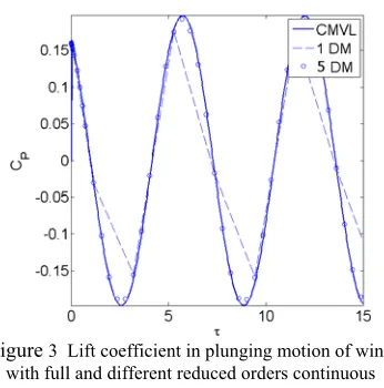
At first, the validity of aerodynamics model, in continuous time form is investigated. For this purpose the non-dimensional lift coefficient of wing in plunging motion calculated from discrete and continuous form of the full order modified vortex lattice aerodynamic models (Eqs. 18 and 22) are shown in Fig. 2. In this figure, results obtained form discrete and continuous time equations are shown with solid and dash lines, respectively. As seen from this figure, there is good conformity between these results.
Figure 2 Lift coefficient in plunging motion of wing with full order discrete (solid line) and continuous
time (dash line) modified vortex lattice models.
Figure 3 Lift coefficient in plunging motion of wing with full and different reduced orders continuous
time modified vortex lattice models.
After examinations of the continuous time modified vortex lattice model for simple calculations, the aeroelastic characteristics of the model are considered here.
With excluding the nonlinear structural term of
F
Nijfrom Eq.(13), and its combination with Eqs. 22 and 24 linear aeroelastic models will be obtained. Calculation of eigenvalues of these linear equations with increasing free stream velocity, determines the stability of the linear aeroelastic system. Figs. 4 and 5 show these eigenvalues for continuous time full and reduced order modified aerodynamics models, respectively. There are two intersections of
Re(
λ
i)
with the velocity axis. One at UF= 42m/s for critical flutter velocity and the other is Ud=
54.3m/s for divergent velocity. As seen from these figures, results obtained from reduced order aerodynamics model are similar with full state aerodynamics model. The results of this section are in complete agreement with results given by [10].
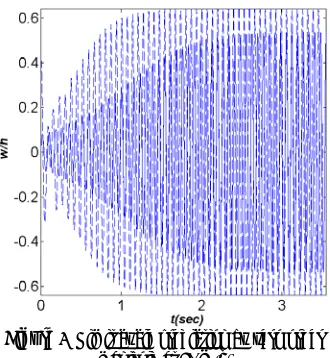
Now the validity of the nonlinear aeroelastic equation of motion in full and reduced order aerodynamic cases are investigated (Eqs. 13, 22 and 24). For this purpose, the transverse displacement of the aeroelastic model with full and reduced order aerodynamics models at a velocity of
60m/s (greater than the flutter velocity) is shown in Fig.6. As seen from Fig.6, the nonlinear aeroelastic model at this velocity undergoes a limit cycle oscillation and the results obtained from full and reduced order aerodynamics models are completely the same. This result is in conformity to the result given in [10].
4.2 Centre Manifold Results
After investigating the validity of the aeroelastic model, the results obtained by applying the centre manifold method are presented.
Figure 4 Eigenvalue solution of open loop linear aeroelastic model with full order continuous modified vortex lattice model.
Figure 5 Eigenvalue solution of open loop linear aeroelastic model with reduced order modified continuous vortex lattice model.
Figure 6 Transverse displacement at 60m/s with full (-) and reduced (--) order continuous time
modified aerodynamics model.
4.2.1 Zero Order Centre Manifold
this approximation all dynamics which are corresponded to J1 dynamics of Eqs.(27 and 28) will be ignored and
only the Jo dynamics with related variables are retained in
the approximation. The obtained zero order centre manifold is given in appendix 6-a.
A comparisons between aeroelastic responses of the original aeroelastic system (obtained by fourth order Runge-Kutta method) [10] and that obtained from zero order centre manifold approximation is shown in Figs.(7). As seen from this figure, there is relatively good conformity between these two results and this simple approximation present very good approximation of this highly nonlinear system.
Figure 7 Limit cycle prediction by zero order manifold at 50m/s.
4.2.2 Third Order Centre Manifold
After using a zero order centre manifold approximation it is reasonable to incorporate second order manifold, but because of the form of the nonlinearity presented in this aeroelastic model these manifolds are not applicable here. Hence here a third order approximation of the centre manifold is used in continuo. In this case, the reduced order system will be in the form given in appendix 6-b. The limit cycle predictions obtained from these manifolds and their comparison with those obtained from time response analysis of Ref.[10] are shown in Figs.(8) and (9).
In [6] Grizedzinski investigated limitations in the application of the polynomial approximation of the centre manifold for predicting limit cycle amplitudes. He showed formal power series expansion used in the method of centre manifold reduction will diverge or cannot predict the occurrence of a stable limit cycle for some cases.
In continuo higher order centre manifold will be used for investigating this limitation. For this purpose a fifth order manifold is used.
4.2.3 Fifth Order Centre Manifold
For fifth order manifolds, the reduced system will be in the form given in appendix 6-b.
Figure 8 Limit cycle prediction by third order manifold (dash line) and original aeroelastic system
(solid line) at 55m/s.
Figure 9 Limit cycle prediction by third order manifold (dash line) and original aeroelastic system
(solid line) at 60m/s.
Figure 10 Limit cycle prediction by fifth order manifold (dash line) and original aeroelastic system
The aeroelastic response obtained from fifth order manifold approximation and its comparison with those obtained from original aeroelastic equations are shown in Figs.(10). As seen from this figure, there are very good approximation between two results. Also, these results are in agreement with those results obtained from third order manifold. These results show in current aeroelastic model the limitation stated by Grizedzinski [6] is not presented.
The bifurcation diagram obtained from zero, third and fifth order centre manifold and its comparison with the bifurcation diagram of the original aeroelastic [10] system is shown in Fig.11. As seen from this figure, zero order centre manifold has relatively good accuracy in comparison with higher order manifolds of third and fifth orders, and with increasing manifold orders convergence of the results are obtained.
Figure 11 Comparison between different bifurcations diagrams of zero (o), third (×) and fifth (□) order
centre manifolds.
5. CONCLUDING REMARKS
In this study, the centre manifold is used for predicting limit cycle amplitude of a highly nonlinear system. Zero, third and fifth order manifolds are used for this purpose and since second and forth order manifold does not give proper results, they are excluded from calculations. Results obtained from calculations show, the zero order manifolds is a nearly good approximation of this highly nonlinear system, and results obtained from higher order manifold, i.e., third and fifth order manifolds give reduced models which completely describe the original very highly nonlinear model. Results obtained from this study can be used for further analysis such as determination of the domain of the attraction of limit cycles and controller design.
6. APPENDIX
a) Reduced model by zero order centre manifold
3 2 2 2 1 2 2 1 3 1 5 2 2 1 3 2 2 1 2 1 21827 0 030496 0 0019018 0 10 1897 4 ) 10 30252 0 10 10535 0 ( ) 29417 0 010645 0 ( 5803 5 w . w w . w w . w . w . w . U w . w . U w . w -− − − × − × + × + + + − = − 3 2 2 2 1 2 2 2 1 3 3 1 6 2 3 1 5 2 2 1 1 2 032114 0 10 45355 0 10 27609 0 10 6975 6 ) 10 53734 0 10 5897 2 ( ) 054743 0 0040673 0 ( 5803 5 w . w w . w w . w . w . w . U w . w . U w . w − × − × − × − × + × + + + = − − − − −
b) Reduced model by third order centre manifold
7. REFERENCES
Periodicals:
[1] E. H. Dowell, J. Edwards, and T. W. Strganac, Nonlinear Aeroelasticity, J. Aircraft, 40 (5) (2003) 857-874.
[2] Liu, L., Wong, Y. S., and Lee, B.H.K, Journal of Sound and Vibration 2002, 234(4), 641-659, Application of the centre manifold theory in non-linear aeroelasticity.
[3] Shahrzad, P. and Mahzoon, M., Journal of Sound and Vibration 2002 256(2), 213-225, Limit cycle flutter of airfoils in steady and unsteady flows.
[4] Dess, D., Mastroddi, F., and Morino, L., Journal of Sound and Vibration 2002 256 (2) 347-365, Limit cycle stability reversal near a Hopf bifurcation with aeroelastic applications.
[5] Dess, D., Mastroddi, F., Journal of Fluids and Structures 2004 19, 765-783, Limit cycle stability reversal via singular perturbation and wing flap flutter.
[6] Grzedzinski, J., Journal of Fluids and Structures 2005, 21, 187-209, Limitation of application of the centre manifold reduction in aeroelasticity
[7] Qian , D., and Li, W. D., Aerospace Science and Technology 2006, 10, 427-434, The flutter of an airfoil with cubic structural and aerodynamic nonlinearities.
[8] Bi, Q.S., Yu, P., Journal of Computer and Applied Mathematics 1999, 102, 195-220, Symbolic computation of normal forms for semi-simple cases.
[9] K.C. Hall, AIAA Journal, 1994, 32 (12) 2426-2423 Eigenanalysis of Unsteady Flows About Airfoils, Cascades, and Wings. [10] D. Tang, E.H. Dowell and K.C. Hall, AIAA Journal, 1999, 37 (3)
364-371 Limit Cycle Oscillation of a Cantilevered Wing in Low Subsonic Flow.
[11] M. Behbahani-Nejad, H. Haddadpour, and V. Esfahanian, Journal of Aircraft 2005, 42 (4) 882-886, Reduced-Order modeling of unsteady flows without static correction requirement
Books:
[12] Dowell, E.H., Aeroelasticity of Plates ans Shells, Kluwer/Noordhoff International Publishing, Leyden, 1975.
[13] Meirovitch, L., Principles and Techniques of Vibrations, Prentice-Hall International INC. 1997.
[14] J. Katz and A. Plotkin 1991, Low Speed Aerodynamics, From Wing Theory to Panel Methods, MCGRAW – HILL ,New York. [15] J. Carr 1981 Application of Centre Manifold Theory, New York,