Two essays on the predictability of asset prices: "Benchmarking problems and long horizon abnormal returns" and, "Low R square in the cross section of expected returns"

University of New Orleans University of New Orleans

ScholarWorks@UNO

ScholarWorks@UNO

University of New Orleans Theses and

Dissertations Dissertations and Theses

5-18-2007

Two essays on the predictability of asset prices: "Benchmarking

Two essays on the predictability of asset prices: "Benchmarking

problems and long horizon abnormal returns" and, "Low R square

problems and long horizon abnormal returns" and, "Low R square

in the cross section of expected returns"

in the cross section of expected returns"

Benito Sanchez

University of New Orleans

Follow this and additional works at: https://scholarworks.uno.edu/td

Recommended Citation Recommended Citation

Sanchez, Benito, "Two essays on the predictability of asset prices: "Benchmarking problems and long horizon abnormal returns" and, "Low R square in the cross section of expected returns"" (2007). University of New Orleans Theses and Dissertations. 1080.

https://scholarworks.uno.edu/td/1080

This Dissertation is protected by copyright and/or related rights. It has been brought to you by ScholarWorks@UNO with permission from the rights-holder(s). You are free to use this Dissertation in any way that is permitted by the copyright and related rights legislation that applies to your use. For other uses you need to obtain permission from the rights-holder(s) directly, unless additional rights are indicated by a Creative Commons license in the record and/ or on the work itself.

Two essays on the predictability of asset prices:

"Benchmarking problems and long horizon abnormal returns"

and,

"Low R square in the cross section of expected returns"

A Dissertation

Submitted to the Graduate Faculty of the University of New Orleans in partial fulfillment of the requirements for the degree of

Doctor of Philosophy in

Financial Economics

by

Benito A. Sanchez

B.S., University of Carabobo, 1993 M.B.A., IESA, 1995

M.A., Tulane University, 2001 M.S., University of New Orleans, 2005

Dedication

This dissertation would not exist without the support of my loved wife, Irma. She supported me not only during the intellectual demanding work that is to write a dissertation, but also during the whole Ph.D. program. For more than 12 years, she has literally lived my previous master degrees and my entire academic career. Irma, this is for you.

Dedicatoria

Acknowledgement

Table of

C

ontents

Abstract ... vi

Essay I: Benchmarking problems and long horizon abnormal returns...1

I. Introduction ...1

II. Literature review ...6

A. Benchmarks for Measuring Abnormal Returns ...6

A.1. Characteristics Based Models ...7

A.2. Factor Models ...9

A.3. Stochastic Discount Factor Models...11

B. Statistical corrections for current methods...13

B.1 Carefully constructed portfolios and skewness-adjusted t statistics ...13

B.2. Bootstrapping ...14

B.3 Calendar time portfolios...15

B.4. Bayesian approach...16

C Seasoned Equity Offerings performance...18

III. Methodology ...19

A. Asset Pricing Benchmarks ...20

A.1 The Stochastic Discount Factor ...20

A.2 Alternative Asset Pricing Benchmarks ...23

A.3 Restricted Asset Pricing Model...24

B Data Description...27

IV. Results...32

A CRSP Sample Distributions ...32

A.1 The Fundamental Benchmarking Problem ...38

A Seasoned Equity Offerings performance ...41

C Predictability of alphas...44

V. Conclusions...56

Appendix A: Derivation of the Restricted Asset Pricing Model (RAPM) ...62

Appendix B: Alternative CAR estimation ...65

Essay II. Low R square in the cross section of expected returns...74

I. Introduction ...74

II. An Empirical Model of the Cross-Section of Expected Returns ...76

A. Time Series and Cross-Sectional R2s ...77

B. Expected return and market return variance ...78

II.2 The error in variable problem...80

C. Data description and estimation procedure ...81

III. Empirical Results ...83

A. Explaining the cross-sectional R2 volatility ...89

B. Time series and cross-sectional R2 in portfolios ...92

List of Tables

Essay I’s Tables.

Table 1. Summary of abnormal returns tests ...17

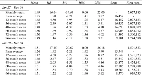
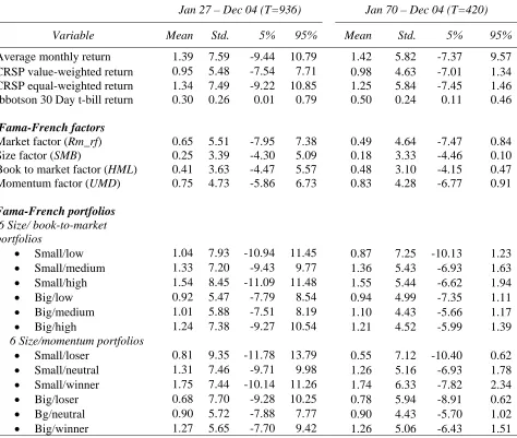
Table 2. Return Descriptive Statistics...30

Table 3. Benchmark model performance...34

Table 4. Sample and SEO pricing with selected Benchmark models...42

Table 5. SEOs’ average CAR decomposition...44

Table 6. Alpha statistics...47

Table 7. Predictability of Jensen’s alphas...47

Table 8. Average Alpha by decile (period: Jan 1970 – Dec 2004)...50

Table 9. Predictability of Jensen’s alphas by decile ...52

Table 10. Alpha Predictability (Transition Table)...54

Table 11. Percentage of SEO events by decile ...55

Essay II's tables Table 1. Monthly statistics and Fama MacBeth cross-sectional regression results ...87

Table 2. Overall and firm level sample statistics with cross-sectional regression results ...88

Table 3. R squares comparison for individual firms...91

Table 4. R squares comparison for portfolios...94

Table 5. Monthly statistics and Fama MacBeth cross-sectional regression results ...97

Table 6. Overall and portfolio level sample statistics with cross-sectional regression results ....98

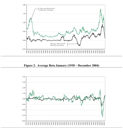
List of Figures Essay I’s figures Figure 1. Average alphas (%, January 1930 – December 2004) ...39

Figure 2. Average Beta January (1930 – December 2004)...39

Essay II’s figures Figure 1. Securities average time series R2 and cross sectional R2 ...84

Figure 2 Market and security average return volatility...85

Figure 3 Behavior of time series and cross-sectional R2 (securities) ...89

Abstract

This dissertation consists of two essays on predictability of asset prices. "Benchmarking

problems and long horizon abnormal returns" and, "Low R-square in the cross section of

expected returns". Long run abnormal returns following Initial Public Offerings (IPOs),

Seasoned Equity Offers (SEO) and other firm level events are well documented in the finance

literature. These findings are difficult to reconcile in an efficient markets world. I examine the

seriousness of potential benchmarking errors on the measurement of abnormal returns. I find

that the simpler, more parsimonious models perform better in practice and finds that excess

performance is not predictable regardless of the APM. Thus, the long run underperformance

following SEOs found in the literature is consistent with market efficiency because excess

performance itself is not predictable.

In the other essay, "Low R-square in the cross section of expected returns", I examine the

“low R-square” phenomenon observed in the literature. CAPM predicts exact linear relationship

between return and betas (SML). This means that estimated time series betas for firms should be

related with firms’ future returns. However, the estimated betas have almost no relationship with

future returns. The cross-sectional R2 are surprising low (3% average) while time series R2 are

higher (around 30 % average). He develops a simple asset pricing model that explains this

phenomenon. Even in a perfect world where there are no errors in the benchmark measurement

or estimation of the price of market risk the difference in R-squares can be quite large due to the

difference in variance between the “market” and average returns. I document that market

variance exceeds the variance of average returns, with few exceptions, for the last 74 years

Keywords: Asset pricing, predictability, cross sectional R square.

Essay I: Benchmarking problems and long horizon abnormal returns

I. Introduction

Most empirical tests of long-run abnormal returns demonstrate anomalous returns behavior.

Long-run is usually defined as a three to five year horizon following an event or set of events

impacting a firm. Abnormal returns are defined as deviations from either a benchmark asset

pricing model or a reference portfolio of matched firms. Negative cumulative abnormal returns

(CARs) indicate “underperformance” and positive cumulative abnormal returns show “superior

performance”.

The phenomenon of long-run underperformance of firm equity returns following a

variety of events such as mergers (Asquith, 1983; Agarawal, Jaffe and Mandelker, 1992),

dividend omissions (Michaely, Thaler, and Womack, 1995), Initial Public Offerings (IPOs) and

Seasoned Equity Offerings (SEOs) (Ritter, 1991; Loughran and Ritter, 1995), and more recently

bond ratings changes (Dichev and Piotroski, 2001) is well-documented in the literature.

Research also documents long-run superior performance following another set of events,

such as, dividend initiations (Michaely et al., 1995), earning announcements (Ball and Brown,

1968; Bernard and Thomas, 1990), open-market share repurchases (Ikenberry et al., 1995;

Mitchell and Stafford, 2001), tendered share repurchases (Lakonishok and Vermaelen, 1990;

Mitchell and Stafford, 2001), and stocks split (Dharan and Ikenberry, 1995; Ikenberry et al.,

1996).

The preponderance of long-run underperformance and superior performance of equity

returns has become a stylized fact in the literature, but these empirical findings challenge the

market efficiency paradigm and are difficult to reconcile with an equilibrium asset pricing

model. Market efficiency (ME) is essential to well-functioning financial markets and is a

fundamental tenant of standard finance models. In a well-functioning financial market,

mis-pricing should not exist for long periods of time. However, empirical findings seem to indicate

there are indeed long periods of misaligned prices. Long periods of mis-pricing violate any

concept of investor rationality.

Long-run abnormal returns studies are plagued with benchmarking errors that raise

doubts about the validity of their findings. Fama (1998) calls using the wrong benchmark asset

pricing model (APM) used to calculate abnormal returns. Under ME, the mean cumulative

abnormal return should be zero, but in the literature this depends on the APM under study.

While Kothari and Warner (1997) find a positive bias in mean cumulative abnormal returns from

the APMs they study, Barber and Lyon (1997) find a negative bias in mean cumulative abnormal

returns for the APM they study. The bias in mean cumulative abnormal returns biases t-tests if

the researcher assumes the asset pricing model is correct (i.e., a mean zero abnormal return).

I examine the seriousness of potential benchmarking errors on an exhaustive set of

benchmark APMs using an expansive collection of individual equity returns from the Center for

Research in Securities Prices (CRSP) from January 1927 through December 2004. The APM’s

performance is measured by computing out of sample mean cumulative abnormal returns over

12, 36, 60 month horizons. I also look at the performance of APMs out of sample under the asset

pricing restriction that intercepts (i.e, “alpha” a measure of ex post excess performance) are zero.

I judge the goodness of fit alternative APMs by looking at the variance of prediction errors

relative to a simple random walk model. The best APMs are selected based on mean and

goodness of fit and studied further. The selected APMs are used to assess SEO performance

reported by Securities Data Corporation (SDC) from January 1970 because SEOs have proven

the most difficult for APMs to price.

This research examines the long run performance of 13 asset pricing benchmarks. The

simplest APMs are the single index models including the Capital Asset Pricing Model (CAPM)

and Market Models (without a risk free rate) using equally weighted and value-weighted CRSP

market indices. The performance of ad-hoc Fama and French three (market, size,

book-to-market) and four (market, size, book-to-market and momentum) factor models that have become

common place in the finance literature are also examined.

In addition to the standard finance models, I study the long-run abnormal return

properties of a benchmark “free” model based on Hansen and Jagannathan (1991)’s stochastic

discount factor (SDF). The main advantage of the SDF is that it encompasses all rational asset

pricing models (e.g., it does not require a specific asset pricing model to estimate expected

returns). The SDF is the least subject to the bad model problem as it imposes the least

restrictions on the behavior of asset prices. Similar to Arbitrage Pricing Theory, the number of

believed to convey pricing information are used to form six different SDF benchmarks. The

underlying assets are the same assets used in forming Fama and French factors.

The last model I study is created as part of this research. This is a variant of the CAPM

which avoids what I call the “fundamental benchmarking problem.” This model imposes a

natural condition found in most principles of finance texts. This condition states that there is no

idiosyncratic risk in the aggregate. For a given set of assets defined as “the market” this is

tautological, where the average market beta must be one and average market excess performance

(alpha) must be zero. In other words, the market cannot outperform the market. However in

most studies a sub-set of assets are of interest and this condition does not hold by definition.

Using the large collection of assets in the study, I impose the restriction that guarantees there is

no market wide miss-pricing and examine its performance along with other APMs.

The simpler, more parsimonious models perform better in practice. The relative mean

square error indicates that models which use an equally weighted index perform better than those

that use a value-weight index. The CAPM (equally –weighted) marginally outperforms the other

single index models including the restricted CAPM I propose. The out of sample performance of

these models indicates that the CAPM-EW can reduce prediction variance relative to a naïve

random walk model by 15-20%. The more complicated SDF benchmarks perform miserably out

of sample. Even though the SDF benchmark uses the same information that is contained in

assets forming the Fama and French factors, the Fama and French three and four factor models

perform much better. The Fama French 3-factor model seems to outperform its four factor

counterpart.

For every APM tested, imposing the asset pricing restriction that APM predictions

exclude their intercepts results in better performance than assuming excess performance

continues into the future. This indicates that excess performance may not be predictable

regardless of the APM.

Excluding the SDF benchmarks, all of the common APMs suffer from the “bad model

problem” as the average excess performance in these models is positive. That is the average

security outperforms the market! I show this is because low performing firms (negative alpha)

do not survive in the dataset as long as higher performing firms.

Based in lowest absolute mean cumulative abnormal return predictions, the equally

cumulative abnormal returns using intercepts in prediction also perform better than those that do

not. If a researcher uses intercepts in their prediction then the population mean cumulative

abnormal return should be assumed to be slightly negative and if a researcher does not use

intercepts in their predictions then the population mean should be assumed positive.

Of all the APMs, the restricted APM I propose does best on balance considering mean

and variance of predictions.

Next I use the selected models, CAPM-EW the restricted CAPM, Fama French three and

Fama French four factor models to study the long run performance of SEOs. While the degree of

mis-pricing among models is very similar, the degree of mis-pricing with and without the asset

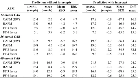
pricing restriction in benchmark predictions is striking. At 12 months after an SEO, using

intercepts in predictions reveals that SEOs under perform by 14% or more. With the asset

pricing condition in place, the degree of underperformance drops to about 5%. At 36 months

after an SEO, the mis-pricing under the asset pricing restriction is about 16% which is half as

much as with using intercepts in benchmark predictions. These results indicate SEOs are

initiated by firms with disproportionately high ex post excess performance (i.e., high alpha

firms). As SEOs demonstrate, investors expecting high excess performance to continue will be

badly mistaken.

The true degree of miss-pricing is not contained in the mean abnormal returns, but in the

measure of excess performance. As firms issue equity, leverage declines and firms’ betas also

decline. Thus some of the abnormal returns difference can be explained by changes in risk

sensitively over the horizon under examination. Indeed, I do find a decline in betas of SEO firms

after issuance, however underperformance still exists.

I examine the predictability of excess performance. The evidence presented thus far

would suggest that SEOs are overpriced, but if in the months after an SEO, a securities excess

performance is not predictable there would be no way to take advantage of any overpricing. I

find very weak predictability from relating measures of excess performance of selected APMs to

their past. The R2 from these regressions are under 2%. Given there has been an SEO, the future

excess performance is significantly lower, but it is extremely uncertain as demonstrated by the

2% R2. I also find that SEO firms are high alpha firms; however this is not a homogenous group.

Firms in the lowest deciles of performance also participate in the SEO process and have higher

the lowest decile 36 month later. Like the population of CRSP securities under study, SEO

excess performance appears independent of its past. The negative mean abnormal returns of

SEOs seem to be related to some extreme negative performing securities in months after

issuance, but not a characteristic of SEOs themselves.

The remainder of this study is divided as follow. Section II reviews the literature of

measuring long-run abnormal returns and summarizes the SEO literature. Section III describes

the data and presents the methodology used to compute cumulative abnormal return for the set of

II. Literature review

Measuring abnormal returns is difficult as they are defined as deviation from a “true” asset

pricing model. Market Efficiency (ME) rejections may be caused by a misspecified model and

have little to do with ME itself. Fama (1998) calls using the wrong benchmark asset pricing

model to assess ME the “bad model problem.” The bad model problem is especially severe in

long run abnormal returns because model errors are cumulative. Fama (1998) states that

consistent with the ME predictions, most long-term anomalies tend to disappear “with reasonable

changes in technique.”

Long run tests of ME are not only plagued with potentially severe benchmarking error, but also

with statistical difficulties. For example, standard inference using t-statistic depends on

normality and independence. Long abnormal return studies show abnormal returns are positively

skewed and suffer both contemporaneous correlation and time series dependence. Whether these

statistical properties are part of the nature of abnormal returns or arise from “bad” models is an

open question.

This section reviews the different approaches to test long-run abnormal performance.

Specifically, it reviews all benchmarks models used in the literature as well as the statistical

difficulties and proposed solutions to current tests of long-run abnormal return.

A. Benchmarks for Measuring Abnormal Returns

In the literature, abnormal returns are pricing errors or return deviations from a well defined

benchmark. The benchmark is either an asset pricing model or a reference portfolio of firms

with similar characteristics as the set under study. The abnormal return:

ARi = Ri – Bij (II.1)

is the difference between firm i’s return Ri and the return of the benchmark Bij (time subscript

suppressed for clarity), where j is either a reference portfolio (mp), a control firm (cf), or an asset

pricing model (APM). The benchmark for firm i, B_ij =

{

(

)

}

Define abnormal performance by cumulative abnormal returns (CAR):

∑

∑

=

τ τ

τ ( , )

, i i ij

i AR R B

or by differences in returns from buy and hold strategies:

∏

∏

τ τ

τ (1 ) (1 )

, i ij

i R B

BHAR , (II.2.b)

over the performance period τ.

The significance of abnormal performance uses the t-statistic:

N S

CAR t

CAR

= , or

N S

BHAR t

BHAR

= . (II.3.a, II.3.b)

where CAR and BHAR are the cross-sectional means of N event firms, and, S_CAR and S_BHAR

are their respective standard deviations. Statistical inference based on this test requires that

abnormal returns are independently distributed normal variables.

A.1.Characteristics Based Models

Characteristics based models have a long tradition in long horizon studies. The main advantage

of the characteristics based approach is that it does not rely on a particular asset pricing model to

define benchmark returns. The benchmark for measuring abnormal returns for each event firm

uses returns from either a single or set of “like” firms. A “match” for each event firm is found

by selecting firm(s) based on similar “characteristics.”

Admittedly, characteristics based models are ad hoc and do not have to be risk based.

Characteristics are any set of criterion that produces separation in average returns.1 The most common approaches are “reference portfolio” and “control firm”.

a) Reference portfolios

Characteristics based portfolios are commonly used benchmarks that have evolved. The earliest

studies used equally or value weighted market indices as benchmark portfolios. After the

seminal works by Fama and French (1992, 1993), reference portfolios became more refined by

matching on size and book-to-market ratios. After Jegadeesh and Titman (1993), momentum

1

became an additional criterion. The benchmark return becomes the realized return of the

characteristics based portfolio for event firm i: Bij = Ri,mp.

However, Barber and Lyon (1997), and Kothari and Warner (1997) identify potential

biases of using reference portfolios. The new listing bias arises because the sample firms under

study usually have a long pre-event return record, whereas the benchmark portfolio may include

recent IPOs which are known to have abnormally low returns (Ritter, 1991; Loughran and Ritter,

1995). Second, the rebalancing bias arises because the compounded return on the benchmark

portfolio implicitly assumes periodic rebalancing of the portfolio weights, whereas it is not

possible to rebalance single event firm returns. Finally, the skewness bias arises because

abnormal returns are not normally distributed. The single event firm return cannot take

advantage of the Central Limit Theorem properties that apply to firms combined into the

reference portfolio. The consequence is that event firm returns are skewed to the right while

portfolio returns converge to normality. Those biases reduce the size of t-test of abnormal

returns resulting in more frequent rejections than expected under the conventional t-distribution.2

b) Control Firm

In the control firm approach, event firms are matched to a particular “control” firm based on

characteristics such as size, book-to-market ratio, and –more recently– momentum. The

benchmark return becomes the realized return of the control firm for event firm i: Bij = Ri,cf.

Barber and Lyon (1997) show the control firm approach alleviates reference portfolio

biases. The control firm benchmark eliminates the new listing bias because the control firm must

exist during the performance period. This approach also eliminates the need for rebalancing

because a single control firm return is the benchmark instead returns of a portfolio. Finally, this

approach mitigates the skewness bias because both the event firm and the control firm are

equally likely to experience large positive returns.

The control firm approach is not a panacea free of empirical difficulties. Lyon, Barber

and Tsai (1999) provides evidence that the control firm approach does not work well if event

firms appear multiple times in the same performance period, if event firms are large, if event

firms are from the same two (or three)-digit SIC industry, or if event firms have large pre-event

2

momentum. This is problematic because most firm events under study (i.e., IPOs, SEOs, Stock

Repurchases, and other corporate events) are likely to satisfy one or more conditions under

which the control firm approach suffers shortcomings. Additionally, the criteria to choose the

control firm are subjective resulting in potentially different results when choosing different firms

to study the same event.

Furthermore, most firm level events are neither cross-sectional nor time independent and

that causes statistical inference problems. Corporate events empirically tend to bunch together in

“hot” periods introducing cross-sectional correlation. Also, empirically firms have multiple

events in short periods; violating time-independence. Thus, the control firm approach is very

limited in its application: it is only appropriate if the arrival of firm events is random and firms

do not have multiple events in the same performance period, which is not the case on many

corporate events.

A.2.Factor Models

An alternative to using matched firms returns, as a benchmark for abnormal returns is to define

benchmark returns as predictions of an asset pricing model (APM). Matched firm returns are

“model free” in the sense that these benchmarks do not need the parameterization of particular

APM, but they do require the characteristics of matched firms to be specified. The advantage of

parameterizing a specific APM is that a consistent set of restrictions on asset pricing behavior

can be imposed (i.e., in the cross section of returns). An APM is attractive not only because of

its theoretical appeal, but also because of the universality of its application. Abnormal

performance in the context of a particular APM is defined intuitively as the difference between

an event firm returns and its predicted return given an event firm’s exposure to systematic risk.

Essential to the APM approach is the implicit assumption that the asset price model under

consideration correctly price assets (see for example, Davis, Fama and French, 2000, and Daniel,

Titman and Wei, 2001). In other words, the implied assumption is that factors and or

characteristics chosen by researchers do indeed describe the cross-section of expected returns.

Fama (1998) argues that most tests for long-run abnormal return suffer from the “bad” model

problem where the magnitude of abnormal returns is rarely robust to alternative methodologies.

Moreover, Fama emphasizes that APMs, by their nature, are necessarily incomplete descriptions

The Fama-French (FF, 1993) three factor model is the most widely used APM in the

literature where expected returns are generated by a market factor, a size factor, and a

book-to-market factor.3 The FF regression model as applied to post event monthly returns is,

( ) 1...

it ft i i mt ft i t i t it

R −R =α β+ R −R +s SMB +h HML +ε i= n, (II.4)

where Rit is the return of event firm i, Rft is the risk free rate, Rmt is the value-weighted market

index return, SMBt is the return of arbitrage portfolio that is long in valued-weighted small stocks

and short in a valued-weighted portfolio of big stocks, HMLt is the return of arbitrage portfolio

that is long in valued-weighted high book-to-market stocks and short in a valued-weighted

portfolio of low book-to-market stocks.4 The factor loading are βi, si, and hi. The error term is

εit. Regressions are run separately for a set of n event firms to obtain a set of αi’s which are

Jensen’s measures of abnormal performance.5

The cross-sectional average of alphas is calculated and a t statistic is used to test the null

hypothesis of no abnormal return. Thus,

1

/

N i i

N

α α

=

=

∑

N S t

/ α

α

= , where

Sα is the cross-sectional standard error.

As Barber and Lyon (1997) emphasize, this method has two advantages. First, it does not

require book-to-market data for the sample firm, allowing firms without available data for size

and book-to-market ratio to enter the analysis. Second, because the model does not require an

explicit measure of size and book-to-market, it can capture patterns that would otherwise be

miss-categorized (e.g., large firms that behave like small firms).

More recently, a fourth “momentum factor” has been added to the FF specification.

Jegadeesh and Titman (1993) show that an arbitrage portfolio that is long on past winners and

short in past losers earns a positive return that is not captured by FF’s three factors. Thus, the

amended FF model includes an additional factor risk; the momentum effect. The regression

setup is the same as above,

3

Womack (1996) used this method to study long-run analyst recommendations, and Loughran and Ritter (1995) used it to study Initial Public Offerings and Seasoned Equity Offering.

4

Fama-French factors have become a standard in the finance literature. A detailed description of how this factor are constructed can be found in Fama and French (1993) and the K. French’s website:

http://mba.tuck.dartmouth.edu/pages/faculty/ken.french/ 5

( ) 1 1...

it ft i i mt ft i t i t i t it

R −R =α β+ R −R +s SMB +h HML + p PR YR +ε i= t (II.5)

with an additional regressor PR1YR that accounts for momentum. PR1YR is the Jegadeesh and

Titman (1993) arbitrage portfolio. Studies of long-run abnormal returns follow Carhart (1997) in

constructing the momentum factor. Carhart constructs this variable first by computing the

average return on all firms in the last eleven months. The arbitrage portfolio return is then

formed by taking the difference between equally weighted portfolios of firms with the highest

(top 30%) past returns and firms with the lowest (bottom 30%) past returns. The testing

procedure using cross-sectional alphas follows the same manner as in the three-factor case.

The FF three and four factor versions have disadvantages beyond the “bad” model

problem. These APMs assume parameter stability that could be a problem in studying long-run

horizons (5 years). Over longer horizons, there are more opportunities for a firm to change size,

book-to-market ratios and other characteristics. In addition, the time-dependence and/or

cross-sectional correlation of abnormal returns can bias the inferences.6

A.3.Stochastic Discount Factor Models

The stochastic discount factor (SDF) approach to benchmarking returns was first suggested by

Chen and Knez (1996) who built on the work of Hansen and Jagannathan (1991). The SDF is

model free in the sense that it requires only that the law of one price holds. Expected returns can

be computed with the first two moments of return data without assuming a specific utility

function, complete markets, normality of returns or that a particular benchmark portfolio is a

tangency portfolio. Therefore the SDF model is well suited to address the bad model problem as

it imposes the least restrictions on the behavior of asset prices.

Early theoretical development of the SDF is credited to Ross (1978), Rubinstein (1976),

and Harrison and Kreps (1979). The SDF is constructed on the principle that the law of one

price holds. The law of one price is the familiar present value relation,

[

]

= t t t E m x

p (II.6)

where p is a vector of today’s prices on n assets and m is the discount factor that applies to

tomorrows payoffs, x. The law of one price simply states that if two assets have the same set of

6

payoffs they must sell for the same price. This implies there is only one discount factor at each

date.

Hansen and Jagannathan (1991) show that a valid discount factor, m, can be formed as a

linear combination of the returns, mt =b′Rt, where b is a vector of parameters and R is the

vector of gross returns on n assets. Divide (6) through by prices to get:

[

]

E , (II.7)

and substituting the expression for m we obtain

[

]

E . (II.8)

It is straightforward to compute b. The resulting SDF m will exactly price the assets used

in its construction. Hansen and Jagannathan (1991) further prove that the resulting SDF has the

lowest variance of any candidate discount factor and shows there is a duality of the Hansen and

Jagannathan bounds that they develop and the mean variance frontier. The SDF approach

guarantees that resulting portfolios used as benchmark assets will in fact lie on the mean variance

frontier. There are other representations of the SDF that are equivalents. Specifically, discount

factors, betas representations and mean-variance efficient frontier are equivalents, as all of them

carry the same information (Cochran, 2001, p. 101).7 In the SDF context over and under pricing is defined by,

$

1−E mR( _p)=α (II.9)

where Rp is the event firm portfolio and α$ is the parameter of interest. If alpha is greater than

zero there is over pricing and if alpha is negative there is underpricing. Ahn, Cliff, and

Shivdasani (2003) study the long-run performance of SEOs using the moment conditions:

, $

1 '

1 '

t t

p t t

R R b E

R R b α

−

⎡ ⎤

=

⎢ _{− −} ⎥

⎣ ⎦ 0. (II.10)

The discount factor is formed from the set of basis assets. The second moment condition uses

this discount factor to price an event firm portfolio (i.e., α$ =0). The parameter of interest is

7

alpha, which is zero under the null hypothesis. Moreover, GMM can be used to estimate the

parameters.

The main disadvantages are that the approach as presented assumes parameter stability and that it

also is estimated in sample, forcing the pricing errors to be zero by construction.

B. Statistical corrections for current methods

Several approaches exist in the literature to deal with the biases in abnormal return estimation,

the cross-sectional/time series dependence of abnormal returns, and the non-normality of the

abnormal return distribution. These approaches include “carefully constructed portfolios”,

“adjusted test statistics”, “generated empirical distributions”, and “calendar time portfolios”.

B.1.Carefully constructed portfolios and skewness-adjusted t statistics

Lyon, Barber and Tsai (1999) advocate the use of “carefully constructed portfolios” (CCP)

where firms matched by characteristics (size and book-to-market, etc.) are purged of new listings

and portfolios are constructed to avoid rebalancing. The benchmark CCP return is computed by

averaging the compounded individual security returns over the performance period given by:

Bij=

,

1

[ (1 ) 1]

s

s

n i t

bh t s

i s R B n τ + = = + −

=

∑

∏

where ns is the number of stock trade at the beginning of month s. The return of this portfolio is

a passive equally weighted investment in the stocks that constitute the reference portfolio. There

is no investment in new listed stocks after s, nor is there a need to rebalance the portfolio. The

abnormal return in this context is the difference between the buy and hold return of an event firm

i and the CCP return Bij.

Skewness bias will remain even when using CCPs. A researcher may try to correct this

bias using the conventional skewness-adjusted t statistic (Johnson, 1978):

2

1 1

ˆ ˆ

3 6

sa

t n S S

n

γ γ

⎛ ⎞

= _⎜ + + _⎟

⎝ ⎠, (II.12)

where, ( ) AR S AR τ τ σ

= and

However, Lyon et al. (1999) find that, while better than the conventional t-statistic, the

adjusted t-statistic is negative biased, resulting in more rejection of the null hypothesis than

expected. Thus, using the skewness-adjusted t statistic with CCP will not yield well-specified

tests.

B.2.Bootstrapping

Most tests of abnormal performance are based on the normality and independence of abnormal

returns. Bootstrapping procedures can mitigate errors in statistical inference caused by

non-normality of abnormal returns. A researcher may bootstrap the skewness-adjusted t statistics or

the average cumulative abnormal return.

a) Bootstrapped skewness-adjusted t statistic

Lyon et al. (1999) advocate the use of bootstrapped adjusted t statistics to deal with the

skewness bias, regardless the reference portfolio used. They find that “only the bootstrapped

application of the skewness- adjusted t-statistic yields well-specified test statistics.”8

Specifically, take 1,000 bootstrapped re-samples from the original sample of size nb = n/4. In

each resample calculate the skewness-adjusted t statistic (equation II.12). Take the bootstrapped

distribution of tsa and estimate the critical values xl and xu for a significant level α by solving:

( ) ( )

2

b b

sa l sa u

P t ≤x =P t ≥x =α . (II.13)

This method alleviates the non-normality of abnormal return and yields well specified

test. However, as Lyon et al. (1999) recognize, this method fails when there are overlapping

events, which is the case in most long-run abnormal return studies.

b) Bootstrapped empirical distribution of abnormal return from pseudo portfolios

Some researchers have bootstrapped an empirical distribution of average long run abnormal

returns.9 The work of Ikenberry, Lakonishok, and Vermaelen (1995) and latter amended by Lyon et al. (1999), propose replacing every event firm in the original sample with a control firm

8

They mention that these results are consistent with Sutton’s (1993) recommendation. 9

drawn randomly from a set of non-event firms with the same size and book-to-market ratio.

Next, calculate the abnormal return on each control firm as the difference between its holding

period return and the buy and hold return of a CCP (equation II.11). Take the average of

abnormal returns across control firms and record this value. Finally, generate a distribution of

long run average runs by repeating this procedure 1000 times. The researcher compares the

average abnormal return with the percentiles from the empirical distribution.

Bootstrapping the empirical distribution of abnormal return results in more powerful tests

than using a conventional t-statistic. However, as emphasized by Brav (2000), this approach has

two shortcomings. If the two samples (sample of test assets and sample of control assets) have

different variance, the generated empirical distribution will be biased. Second, if the original

sample of event firm returns are cross-sectional correlated, which is most likely the case, the

replacement with random samples may lead to false inferences because the latter assumes

independence by construction. Mitchell and Stafford (2001) present simulation evidence that the

bootstrapped empirical distribution method fails in the presence of cross-sectional and time

series dependent abnormal returns. They find that bootstrapped estimated t statistics could be as

much as four times too large in the presence of zero abnormal return.

B.3.Calendar time portfolios

One shortcoming of using any of the above approaches to testing abnormal returns is the

potential for cross sectional dependence among event firms. Brav (2000) argues that due to

industry effects or other contemporaneous cross firm connections abnormal returns are

cross-correlated. However, most tests of abnormal returns assume independence. Fama (1998)

suggests the use of calendar time portfolios (CTP) to resolve the problem. Sample firms enter

the CTP in the month following the event of interest and are held in this portfolio CTP for five

years, depending on the definition of the long run. The concerns about cross-sectional

dependence are alleviated because this approach eliminates the need to compute and test average

abnormal returns. Instead, the researcher examines the properties of the CTP. Any APM or

characteristic model can serve to benchmark CTP returns.

The most commonly used benchmark for CTP returns is the FF three factor model

Brav and Gompers (1997), and Jegadeesh (2000)]. The CTP return, Rctp, is used to estimate the

three factor regression:10

(

)

p p f

ctp R R R s SMB h HML

R − =α +β − + + +ε , (14)

where the parameter alpha, αp, is the measure of abnormal performance. Lyon, Barber and Tsai

(1999) show that the CTP work well when cross-sectional dependence is severe. However,

because the benchmark itself is subjects to its own problems miss-pricing can persist.

Loughran and Ritter (1999) criticize the use of calendar-time regressions. Through

simulations, Loughran and Ritter find the CTP approach has low power to detect abnormal return

because this approach does not treat “hot” and “cold” event periods differently. In contrast,

Mitchell and Stafford (2000) revisit Loughran and Ritter (1999), accounting for

heteroskedasticity caused by calendar clustering, and find the CTP approach is more powerful in

detecting abnormal return than using bootstrapped reference portfolios.

B.4.Bayesian approach

Brav (2000) proposes a methodology to test long run abnormal return that confronts both

non-normality and cross-sectional dependence of abnormal return. Using a Bayesian approach in a

seemingly unrelated regression (SUR) setting, an empirical testing distribution is generated.

Specifically, given an asset pricing model and a researcher’s prior belief regarding the

distribution of a firm residual, the asset pricing model’s parameters are estimated through Bayes’

theorem. Then, given the estimated parameters, long-run returns for all firms are simulated

taking into account the variance-covariance of the residuals. These steps are repeated a large

number of times, and the simulated averages are used to build the empirical distribution of the

sample mean. Finally, the observed abnormal return is compared with the null distribution.

This approach solves both the non-normality and independence assumption of earlier

approaches. Also, it is neither subject to the new listing bias nor the rebalancing bias because

Brav uses CCPs. However, as Brav (2000) recognizes, it still relies on an asset pricing model or

a particular set of characteristics.

Table 1 shows a summary of current approaches and their advantages and disadvantages.

10

Table 1. Summary of abnormal returns tests

Panel A. Early Approaches

Approach Advantages Shortcomings

Reference Portfolio and

t-statistics

Does not need an asset pricing model Subject to new listing bias, rebalancing bias, skewness bias.

Assume Normality and Independence of abnormal returns.

Control Firm and t-

statistic

Does not need an asset pricing model Works well in random sample

It does not work well when sample firms are large, are from the same set of 3 digit SIC, or have large-pre event momentum. The researcher chooses the reference firm making it depend on researcher

subjectivity.

Asset Pricing Models (regressions)

Neither factors nor characteristics of the test asset are needed to assess abnormal return. Only portfolios with the factors and/or characteristics are needed.

Assume factor loadings are constant over time.

Assume pricing errors are uncorrelated and independent.

An asset pricing model is needed.

Panel B. Improved approaches

Approach Advantages Shortcomings

Carefully constructed portfolios and adjusted t

statistic

Eliminates new listing bias and rebalancing bias.

The skewness bias remains.

Bootstrapped skewness- adjusted t statistic

Take into account the skewness bias Well- specified in random samples

Does not correct cross-sectional

dependence and neither does overlapping events

It is well specified for random events, but not for non-random events.

Bootstrapped empirical distribution of

abnormal return from pseudo portfolios

Well specified if carefully constructed portfolios are used and rebalancing is not allowed.

Underlying assumptions are that event firm and matched firm are similar in every dimension and there is no cross-sectional correlation in sample firms. Test misspecified because of the independency assumption.

Calendar time portfolios

Well specified when there is cross-sectional correlation

More statistical power after controlling for sample composition

Well specified for random sample, but not for non-random samples,

By averaging, it gives the same weights to high intensity events and low intensity events

An asset pricing model is required Bayesian approach Corrects non-normality of abnormal

returns, cross-sectional dependence and time-series dependence.

C Seasoned Equity Offerings performance

Studies of long-run performance following Seasoned Equity Offerings (SEO) have led to

intensive discussion in the literature whether the market efficiency holds or not. Ritter (1991),

Loughran and Ritter (1995), and Spiess Affleck-Graves (1995) find that Seasoned Equity

Offerings (SEOs) underperform market indexes after three and five years after the issuance.

(Loughran and Ritter, 1995). Loughran and Ritter (2000), and Jegadeesh (2000) confirm those

findings. This set of authors argues that the underperformance is due to the effect of investors’

sentiment on returns. Investors who purchase shares in IPOs and SEOs systematically over-value

the shares at the time of issuances.

In contrast, Brav and Gompers (1997), and Brav, Geczy and Gompers (2000) show that

stock returns after IPOs and SEOs follow a more pervasive return pattern for small stocks.

Specifically, Brav and Gompers (1997) find that documented “IPOs underperformance” is not an

IPOs effect, but a firm size effect. Non-issuing small firms tend to have the same

underperformance as issuing small firms (Brav and Gompers, 1997). Moreover, Brav et al (2000)

show that the SEO underperformance is primarily concentrated in small issuing firms with low

book-market ratios. This set of authors argues that the documented underperformance is not

evidence against the ME. Small firms’ issuances are more likely to be held by individual

investors (rather than institutional investors), who are more likely influenced by fads or are

victims of asymmetric information. Once size is taken into account by using valued weighted

returns in benchmark portfolios, the documented underperformance reduces substantially.

Brav et. al. (2000) and Mitchell and Stafford (2001) also show that the reported

underperformance is sensible to the benchmark model, agreeing with Fama (1998)’s bad model

problem. However, Loughran and Ritter (2000) argue that the benchmarks selected by Brav et

al. (2000) and Mitchell and Stafford (2000) incorporate miss-pricing proxies rather than true risk

factors and therefore those miss-pricing proxies bias the test statistics to find no abnormal return

III. Methodology

This dissertation examines the seriousness of potential benchmarking errors in the measurement

of abnormal returns in several methodologies that use a particular asset pricing model (APM),

(including the Stochastic Discount Factor (SDF), which does not assume a particular benchmark

asset-pricing model). The benchmarks use monthly-updated parameters versions of different

asset pricing models (APMs) out of sample. Cumulative abnormal returns (CARs) for all firm

months available from 1927 to 2004 are computed for each APMs. All firm months encompass

the CRSP’s available common stock with at least 37months of return.

Alternative APMs such as market models (MM), capital asset pricing model (CAPM),

Fama and French three factor model (FF3), the Fama and French four-factor (FF4) model, and

the restricted asset pricing model (RAPM), which is a method I propose to force the benchmark

to price itself, are examined herein to asses whether it is the nature of data that is driving

statistical complexities found in the literature. I also obtain CAR under the random walk (RW)

in order to compare the performance of the APMS and SDFs relative to the RW. The literature

has not yet examined the reliability of the RW, FF4, or SDF benchmarks in detecting long run

abnormal performance.11

This research contributes to the literature a study on the properties of the

monthly-updated parameters versions of APMs out of sample. A common critique of benchmark APMs is

that they are constant parameters. The literature has not yet examined the properties of the

monthly-updated parameters parameter versions of alternative APMs. In addition, most research

is conducted in sample with no verification of how alternative models actually perform out of

sample.12 Estimating parameters in sample has the potential problem of forcing pricing errors to be zero, whereas the average pricing error estimated out of the sample is not required to be zero.

I analyze long-run abnormal returns for a set of APMs from January 1930 to December

1999. Previous studies have used shorter periods13. There is no study –to my knowledge– that has investigated the properties of CAR statistics with data spanning this period. I estimate CAR

11

Some authors have used the four factor model as a benchmark to test abnormal return. For example, Brav, Geczy and Gompers (2000) use the Fama-French three factor model and the four factor model and find that the former can capture the joint covariation of IPO returns, whereas the latter is needed to capture the covariation of SEO returns. 12

With the exception of Kothari and Warner (1997) who studies the specification of the market model and FF three factor model with constant coefficients over the performance period. Kothari and Warner (1997) found these two models were severely misspecified.

13

for different sub-periods: 1930-1972, 1973-2004, and 1990-2004. The Center of Research in

Security Price started including NASDAQ common stocks, which are predominantly smaller

companies than the NYSE companies, at the beginning of 1973. Thus, I studied the CRSP

sample pre and post NASDAQ common stock inclusion in the database to see whether the results

are sensitive to this fact. I also calculate CAR statistics for the 1990s because it was

characterized by high volatility in the market.

I estimate CARs for 12, 36 and 60 months using return security data from all available

firms that have at least 37 month of consecutive return in the Center for Research in Securities

Prices (CRSP) database. Previous studies have calculated a random sample of CARS to infer the

CAR statistics. In contrast, I calculate CARs for every firm-month from securities’ returns

during the period January 1927 – December 2004 and report statistics. In other words, for every

firm, I calculate CARS for all valid returns in each firm. There is no study that has estimated

this large CRSP sample that certainly represents the population distribution of CARS. Knowing

the population distribution allows a researcher to use the population mean and standard deviation

to test abnormal return. I also, estimate CARs for under assuming fixed parameters and for

non-overlapping events.

The following sections explain the empirical implementation of SDFs and APMs

considered in this study as well as data sources.

A. Asset Pricing Benchmarks

A.1.The Stochastic Discount Factor

The SDF model is well suited to address the badmodel problem as it imposes the least

restrictions on the behavior of asset prices. This benchmark is considered a model “free” in the

sense that it requires only that the law of one price holds, and expected returns are generated

using the information contained in a set of basis assets rather than a model with pre-specified risk

factors. Furthermore, the SDF encompass all rational asset pricing models, while imposing

fewest restrictions on the ability of assets to price risk. Under the SDF benchmark, expected

returns are computed with the first two moments of the return data without assuming a specific

utility function, complete markets, normality of returns or any other typical assumptions found in

Ahn, Cliff, and Shivdasani (ACS, 2003) is the only other work that studies the long-run

abnormal return using an SDF methodology.14 They find a particular SDF using m=b R' where

m is a SDF, b is a vector of parameters and R is a matrix of basis assets. One shortcoming of

linking m to the data using m=b R' is the possibility that m becomes negative. A negative

discount factor would imply the existence of arbitrage opportunities. ACS impose a

non-negative condition on the discount factor (m>0) but this restriction decreases the robustness of

tests; especially as the number of assets increases. Additionally, they assume the vector b is

constant through time.

Instead of using m as linear combination of basis assets, I use the mean-variance frontier

to test abnormal return as it has the advantage of being intuitive and simple to use in estimation.

Hansen and Jagannathan (1991) prove that a discount factor SDF m=b R' has the lowest

variance of any candidate discount factor and show that there is a duality between the volatility

bounds that they develop and the mean variance frontier. Let Rp and Rop be the return series

from two distinct mean-variance efficient portfolios. The expected return on any event firm i is a

convex combination of any two efficient portfolios:

( )

( )

(

)

( )

E =β + 1−β . (III.1)

Based on this SDF benchmark, I compute long-run abnormal returns from a set of N

event firms over a horizon (T=1, 12, 36, or 60 months) in the following way:

i. Define time indices: Performance period for which abnormal returns is collected

is of length T. The event month is at time k. Define T estimation periods as 36

month windows [k-36, k-1] where k = {1, T} denotes both a particular estimation

period and a particular month when performance is measured.

ii. In each estimation period k, I obtain the vectors of portfolio weights (wp,k, wop,k) of

the efficient frontier assets, Rp, and Rop15

iii. For each estimation period k I obtain the weight β_i,kby running the regression:16

14

ACS apply the methodology to a set SEOs, but they do not study the statistical properties of CARs conditional on the SDF benchmark.

15

Rop is the orthogonal portfolio to Rp when no risk-free asset is assumed and is the 30 day Treasury bill yield when risk-free asset is assumed.

16

(

)

i t op t

i R R R

R, − , =β, , − , +ε t={k-36, k-1} (III.2)

iv. The weights from the tangency portfolios (vectors wp,k and wop,k) and βi,k are used

to obtain a new portfolio that mimics event firm i’s returns for one period ahead

out of sample. The realized return on the benchmark mimicking portfolio, Bi,k, is,

(

)

i k

i R R R

B, =β, , − , + , , k = {1, T} (III.3)

v. The abnormal return is,

k i k i k

i R B

AR_, = _, − _, , k = {1, T}. (III.4)

vi. The cumulative abnormal return for event firm i at time k is,

∑

=

= T

k k i T

i AR

CAR

1 ,

, .

vii. I compute CARs for all firm-months (e.g. all firms i and all months k) available

in the Center for Research in Securities Prices (CRSP) database.17

The SDF benchmark requires the formation of a mean variance frontier for each

estimation period. The choice of assets to be included in the construction of the mean variance

frontier remains an open question. Cochrane (2001) argues that this set of basis assets must be

well motivated because all the pricing information is contained in the variance-covariance

matrix. The literature finds that the market, size, book-to-market (Fama and French, 1992,

1993), and past returns (Jegadeesh and Titman 1993, 2001) are important and nearly independent

characteristics that prices equities. I introduce these characteristics into the covariance matrix of

returns by using the following set of portfolios:

a) The 3 Fama-French factors (market, size, and book to market).

b) The 4 Fama-French factors (market, size, book to market, and momentum)

c) Six size/book to market portfolios and the market portfolio.

d) Augmenting the above set by using six size/momentum portfolios. This means total a

total of 13 portfolios (6 size/book to market portfolios, 6 size/momentum portfolios, and

the market portfolios) to estimate the covariance matrix.

17

I estimate the SDF assuming the existence of a risk-free asset and assuming a zero beta

portfolio for the cases “c” and “d”. Finally, I use the value weighted market index as the market

portfolio.

A.2.Alternative Asset Pricing Benchmarks

The abnormal returns from the RW model, MM, CAPM, FF3 factor model, and FF4 factors

model are computed in a similar way as the SDF benchmark. The RW benchmark is a 36-month

moving average of returns. The RW benchmark,B_iRW_,k , is define as,

36 , 36 1 ,

∑

B , k = {1, T},

and the abnormal prices are measured using,

RW k i k i k

i R B

AR_, = _, − _, , k = {1, T}.

The MM benchmark, B_iMM_,k , uses the regression relation,

t t m k i k i t i R

R, =α, +β, , +ε , t={k-36, k-1},

to determine the benchmark return,

k m k i MM k i R

B, =β, , , k = {1, T}

where αi,k, and βi,k are parameter estimates and Rm is the market return. As in equation III.4,

abnormal returns are defined in excess of the MM benchmark.

The CAPM benchmark uses the regression:

t t f t m k i k i t f t

i R R R

R_, − _, =α _, +β_, ( _, − _,)+ε t={k-36, k-1},

where Rit-Rf is the excess return on the event firm i, Rmt- Rf is the excess return on the market.

The benchmark B_iCAPM_,k uses the estimated beta and the realized Rm and Rf:18

t f k f k m k i CAPM k

i R R R

B, =β, ( , − , )+ , , k = {1, T}.

Abnormal returns are computed as in equation III.4, but in excess of the CAPM benchmark.

18

The FF3 factor benchmark uses the regression specification, t t k i t k i t f t m k i k i t f t

i R R R s SMB h HML

R, − , =α, +β, ( , − ,)+ , + , +ε , t={k-36, k-1},

where Rit-Rf is the excess return on the event firm i, Rmt- Rf is the excess return on the market,

SMB is a zero investment portfolio that is long in small size firms and short in large size firms,

HML is a zero investment portfolio that is long in high book-to-market ratio firms and short in

low book-to-market ratio firms. The parameter estimates βi,k, si,k,and hi,k are the factor loadings.

The , 3

FF k i

B benchmark is:

t f k k i k k i k f k m k i FF k

i R R s SMB h HML R

B_, 3 =β_, ( _, − _, )+ _, + _, + _, , k = {1, T}.

Abnormal returns are computed as in equation III.4, but in excess of the FF3 benchmark.

The FF4 factor benchmark expands the FF3 factor version to include a momentum factor. The

expanded regression relation is,

t t k i t k i t k i t f t m k i k i t f t

i R R R s SMB h HML p PR YR

R_, − _, =α_, +β_, ( _, − _,)+ _, + _, + _, 1 +ε t={k-36, k-1},

where PR1YR is a zero investment portfolio of firms with the highest returns in the last eleven

months minus firms with the lowest returns in the last eleven months (Carhart, 1997). The

parameter, pi,k, is an additional factor loading. The FF4 benchmark returns, , 4

FF k i

B are given by,

k f k k i k k i k k i k f k m k i FF k

i R R s SMB h HML p PRYR R

B , , , , , , ,

4

, =β ( − )+ + + 1 + , k = {1, T}.

Abnormal returns are computed as in equation III.4, but using the FF4 benchmark.

A portfolio can be estimated using equally weighted return or value weighted return. All

benchmarks above use value weighted portfolios to minimize the rebalancing bias. However, I

also investigate the properties of the MM and the CAPM when the market portfolio is calculated

using equally weighted returns.

A.3.Restricted Asset Pricing Model

This dissertation provides evidence that classical asset pricing models used to test abnormal

returns do not price themselves. I call this fact “the fundamental benchmarking problem”.19 In order to alleviate this problem, I propose the restricted asset pricing model (RAPM), which

forces the benchmarking model to price itself.

19

Assume that MM (or CAPM) is an equilibrium model (and therefore market is an

equilibrium priced risk factor). This means that the market portfolio will contain both test assets

and control assets. If the market index is well constructed, the average alpha and beta will be

zero and one respectively. In other words, if firms in the estimation period are exactly the same

in the index (e.g., it is not allowed entering or delisting any firm), then the average alpha and the

average beta are zero and one, respectively.20 To see this let’s R_i be the i firm’s return. Then for each firm i, the market model states:

i m i i

i R

R =α +β +ε (III.5)

where

∑

= = n i i m R n R 1 1

is the market return, n is the number of firms, α and β coefficients, and ε

the error term. The beta coefficient is estimated in a regression as:

(

)

Summing across i , we have

(

)

1 2 1 , cov , cov m m n i i n i m m i n i i R R R R σ σ β ⎟ ⎠ ⎞ ⎜ ⎝ ⎛ = ⎟⎟ ⎠ ⎞ ⎜⎜ ⎝ ⎛ =

∑

∑

∑

dividing by n,

(

)

(

)

1 = = =

⎟ ⎠ ⎞ ⎜ ⎝ ⎛ = ⎟⎟ ⎠ ⎞ ⎜⎜ ⎝ ⎛ =

∑

∑

∑

Therefore, average beta is equal to one. Alpha can be found as:

m i i i R βR

α = −

Summing across i and dividing by n, we have:

(

)

1 1 1 1 1 1 = − = − = − =

∑

∑

∑

∑

i R R R

n R n R R n

n α β β

The results hold for value weighted market portfolio if the weights are fixed during the

estimation period. However, in practice, this will not be true because market value changes

through the estimation period.

20