Print ISSN: 2383-451X Online ISSN: 2383-4501 Web Page: https://jpoll.ut.ac.ir, Email: [email protected]
Capabilities of data assimilation in correcting sea surface
temperature in the Persian Gulf
Abbasi, M.R.1*, Chegini, V.1, Sadrinasab, M.2 and Siadatmousavi, S.M.3
1. Iranian National Institute for Oceanography and Atmospheric Science (INIOAS), Tehran, Iran
2. Graduate Faculty of Environment, University of Tehran, Tehran, Iran 3. School of Civil Engineering, Iran University of Science and Technology,
Tehran, Iran
Received: 22 Oct. 2016 Accepted: 20 Dec. 2016
ABSTRACT: Predicting the quality of water and air is a particular challenge for forecasting systems that support them. In order to represent the small-scale phenomena, a high-resolution model needs accurate capture of air and sea circulations, significant for forecasting environmental pollution. Data assimilation is one of the state of the art methods to be used for this purpose. Due to the importance of thermal structure in monitoring the variations of environmental phenomena, the present study has used Sea Surface Temperature (SST) in data assimilation method to optimize this parameter. SST is one of the most important factors to conduct researches on the ocean, the atmosphere, and their interaction, not to mention monitoring and forecasting air and ocean phenomena as well as commercial and fishing communities and weather forecasts. This study has aimed to present a satellite-derived SST based on pathfinder advanced very high resolution radiometer (AVHRR) data assimilating in FVCOM (finite volume community ocean model) on the Persian Gulf to examine the effect of data assimilation by using the Cressman scheme. The performance of this method has been compared to the optimal interpolation SST (OISST) data, via both visual comparisons and statistical parameters. Applying assimilation method improves correlation coefficient of the model from 0.92 to 0.99. Results demonstrate that the modeled SST has been completely reconstructed by the data assimilated experiment via the Cressman scheme for this region. The spatial and temporal pattern of SST reveals a significant improvement in the entire domain during the investigated period in the gulf.
Keywords: data assimilation, cressman, FVCOM, OISST, SST.
INTRODUCTION
Sea Surface Temperature (SST) has a diurnal range, just like the Earth's atmosphere above, though to a lesser degree thanks to its greater
Corresponding Author Email: [email protected], Tel: +98 9374024737
affect the temperature decrease with height and cloud depth. The lower the temperature, the taller the clouds and the greater the precipitation rate (Barale, 2010). SST is one of the most important factors to conduct a research on the ocean, the atmosphere, and their interaction (Kawai et al., 2006). It is also required to monitor and forecast ocean phenomena, not to mention for commercial and fishing communities (Castro et al., 2001; Li et al., 2010) .
Changes in the thermal structure of water bodies are consistent with changes in the SST in response to climate change and natural variability along with known physical and biogeochemical phenomena in the oceans. Near the coastline, offshore winds move the warm waters towards the surface offshore, replacing them with cooler water from below in a process, known as Ekman transport. This pattern increases nutrients for marine life in the region.
Studying these phenomena rely on accuracy and accessibility of SST maps. Processes such as sediment transport, nutrient distribution, and primary production highly depend on three-dimensional (3D) transport and mixing phenomena, for which the temperature distribution is an essential parameter. Although in situ measurements are the most exact method, scarcity of observational data, use of satellite monitored data is the only option in this regard. Satellite sensors such as Advanced Very High Resolution Radiometer (AVHRR) and
Moderate Resolution Imaging
Spectroradiometer (MODIS) can generate SST for a wide coverage of water surfaces (>1000 km2), involving suitable spatial (~1 km at nadir) and temporal (two times per day) resolutions that cover variations in water temperatures well (Kilpatrick et al., 2015).
Although state-of-the-art coastal models are able to simulate many of the characteristic features of these systems, as well as their statistical occurrence with a reasonable degree of accuracy, the model
simulations tend to contain some errors, due to uncertainty in the initial and boundary conditions and the intrinsic numerical and input data errors.
Inaccurate numerical simulation of the wind, dependent on phenomena like wind waves and wave-induced currents in the Persian Gulf, suffers from lack of offshore wind stations and heat flux data, which is a cause for error in this simulation.
In order to reduce the simulation errors, remotely observed data has been incorporated into the model, using data assimilation. The sparse in-situ surface observations have been complemented with huge amount of data coming from satellites.
the model by means of a nudged optimal interpolation technique.
She et al. (2007) and Larsen et al. (2007) preferred using satellite SST data reconstruction instead of in situ measurements data in the North and Baltic Sea, due to the former's temporal and spatial coverage.
A variety of data assimilation (DA) methods have been developed, such as optimal interpolation (OI), variational method, and ensemble schemes based on Kalman Filter (Chang et al., 2013; Dong et al., 2016). Manda et al. (2005) recognized the skill and feasibility of nudging method, compared to sophistical assimilation methods, such as the EnKF for estimating the upper mixed layer.
In this study, we have used nudging scheme to assess the ability of this assimilation scheme to improve the temperature field structure in a high-resolution setup of a FVCOM model. After the SST assimilation process, the modeled oceanic state variables have been compared with the observed data to evaluate the improvements, yielded by the assimilation procedure.
This paper is organized as the following: First, it briefly describes and evaluates the configuration and performance of the FVCOM model, then to briefly describe the observational data, providing an outline of the nudging in terms of its implementation and technical issues. Afterwards it examines the effects of the SST assimilation on the SST and subsurface temperature profiles. And at the end, it presents the summary and discussion.
MATERIALS AND METHODS
The model, used for this study, is Finite
Volume Community Ocean Model
(FVCOM), an unstructured grid, three-dimensional primitive equation fully coupled with current–wave–ice finite volume community ocean model. This model was originally developed by Chen et al. (2003)
and modified and upgraded by a joint effort of the University of Massachusetts-Dartmouth (UMASS-D) and Woods Hole Oceanographic Institution (Chen et al., 2006). FVCOM is governed by seven primitive equations of momentums, continuity, temperature, salinity, and density in the spherical coordinate; with turbulent mixing, parameterized by the general ocean turbulence model (Burchard, 2002) in the vertical and Smagorinsky turbulent closure scheme in the horizontal (Smagorinsky, 1963). The flux forms of the governing equations are discretized in the unstructured triangular mesh in the horizontal and in the generalized terrain-following coordinate in the vertical (Pietrzak et al., 2002). FVCOM is integrated with options of various mode split and semi-implicit schemes in time and the second-order accurate advection schemes in space. The unstructured grid finite volume methods combine the best attributes of the finite difference method, for simple discrete computational efficiency, and the finite element methods, for geometric flexibility. The flux computational approach provides an accurate representation of mass, heat, and salt conservation.
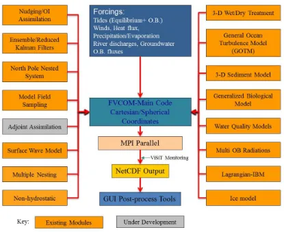
The FVCOM includes a number of options and components as shown in Figure 1.
river inflow used an annual mean transport of 1,576 m3/s with the high-flow season starting from March and continuing until May. The Mellor-Yamada level 2.5 turbulence closure (Mellor & Yamada, 1982) scheme is used for vertical mixing parameterization, while the horizontal diffusion is parameterized by means of Smagorinsky formulation. The external and internal mode time steps are 6.0 and 60.0 s, respectively.
Initially the model was spun up for five years with three hourly-observed wind stress and heat flux as forcing fields, obtained from the European Centre for
Medium Range Weather Forecasts
(ECMWF) reanalysis project, which is going to be referred to as the control run
hereafter. Then for the sake of assimilation, the model spun up with the same setup, though with daily AVHRR SST data.
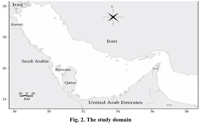
The study period is from 1998 to 2003 and the study area is the Persian Gulf (Fig. 2). The surface forces including daily surface wind, precipitation, evaporation, shortwave, long wave radiation, latent, and sensible heat fluxes, were prepared from ECMWF (European Centre for Medium-Range Weather Forecasts) setup data with 0.5 °C spatial and 6 h temporal resolutions available from 1998 to 2003, containing reanalysis product. To modify and localize the wind data set in the domain, the used results were those of Abbaspour and Rahimi (2011).
Fig. 2. The study domain
Five years of SST data, collected between 1998 and 2003, were selected for assimilation, which had been acquired from the processed AVHRR Oceans Pathfinder project of NASA Jet Propulsion Laboratory (JPL) as well as Physical Oceanography Distributed Active Archive Centre (PO DAAC) due to its low-spatial and high-temporal resolution. Ahmadabadi et al. (2009) showed that the maximum, minimum, and mean error rates for SST in the Persian Gulf were 0.77, -0.09, and ±0.43 respectively, which are acceptable amounts.
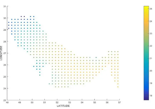
The NOAA Optimum Interpolation Daily SST Analysis 0.25 x 0.25-degree resolution gridded data (Reynolds et al., 2007) (OISST only available from 1982) (Shu et al., 2009) was used in order to verify the assimilation procedure (Fig. 3).
In order to assess the accuracy of the assimilation algorithm and model accuracy, statistical parameters such as the bias, root mean square error (RMSE), and standard deviation between both models were compared with satellite data to estimate the actual influence of the assimilation. This part of the validation process also covered data from different times in different locations of the Persian Gulf. The bias, root mean square error (RMSE) and standard deviation could be calculated as follows:
Bias x y (1)
1
2 2
1 1
n
i i
i
n n
i i
i i
x x y y
R
x x y y
(2)
21
n
i i ε
ε ε σ
N (3)
where, X and Y are the model and satellite data, respectively.
Fig. 3. Locations of the OISST data observation nodes
The Cressman method, as described in the Nowicki paper (Nowicki et al., 2015), is performed as follows: Firstly, the background state 𝑥𝑏 is set equal to the
previous forecast performed by the model. Then the satellite data, used for the assimilation, are stored in the matrix denoted by y. The data, suspected of being invalid because of clouds, the presence of ice, or any other reason, are masked out. The result of the analysis xais then calculated according to Equation (4).
12 1
.
.
nb i
a b n
i
w i j y i x j
x j x j
w i j E
(4)
where i and j represent the satellite and model data grid points respectively, and di j2. is the distance between points i and j. The main parameters of the Cressman method that need to be chosen are the influence radius R and the shape of the weight function w, which determine how the satellite data affect the model. One of the disadvantages of this method is that the influence radius has to be determined by trial and error, causing the parameterization of this method laborious.
After many trials with different sets of the parameters, the one that gave the best
results was chosen. The radius R of the influence was set to 20 grid-points. Beyond that distance, the satellite data weight equaled zero. The weight function in this case would be equal to:
2 2.2 2
. . max 0.
i j
i j
R d
W i j
R d
(5)
RESULTS AND DISCUSSIONS Impacts of SST assimilation
The test of the model was run on the five-year period, from 1998 until 2003. The model assimilation was performed with and without satellite SST respectively, referred to in this paper as assimilation and control run. Results of both runs are compared with each other as well as with satellite data. Validation of the satellite data assimilation with the FVCOM model contained two parts: Firstly, the results of both models were compared with the satellite data to check whether the assimilation algorithm was working properly and to examine the impact of the assimilation on the model results.
Spatial distribution results
Figures 4 and 5 demonstrate the improvement of the FVCOM mean spatial
SST modeling, throughout the study with regards to assimilating the SST data every 24 hours. They illustrate the ability of the DA system to correct SST pattern and systematic model errors, respectively.
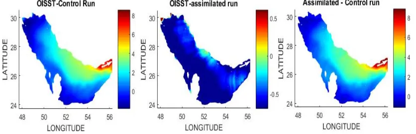
Figure 4 shows that the assimilation run produced a pattern much closer to the OISST. This qualitative consistency is a general feature of the whole SST of the domain. The left and middle of Figure 4 depict the mean difference of OISST and SST model solution from satellite data without and with data assimilation, respectively. The picture on the right shows the difference between the two model runs. The two corners of figure show that the model has difficulties reproducing the observed SST in the Hormuz Strait, while the assimilated model SST agrees much better with the satellite-derived data (middle of Fig. 5).
Fig. 4. Spatial distribution of SST: OISST (left), assimilated run (middle), and control run (right)
Apparently, with SST observational data assimilation, we have reduced the deviation of SST model from the satellite data by more than 7°C. In addition, it can be seen that over most of the northern part of area, the model SST is underestimated in control run, especially in the Strait of Hormuz, while it is overestimated in the southern and shallow region of the domain. In assimilated run, the difference has declined during the study time, even though it has not totally become zero.
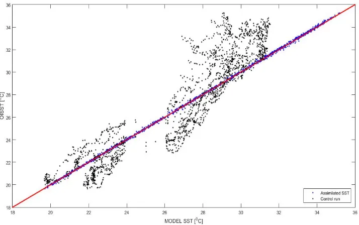
Figure 6 presents a correlation of model data from both cases with satellite measured SST. As can be seen, there is a very strong correlation between all the SST data products from assimilation run and OISST.
Table 1 lists the calculated statistical parameters as described before. The statistics clearly confirm that the assimilation algorithm does improve accuracy. Correlation of the model results with the assimilation makes the satellite data better, and the errors smaller.
Fig. 6. Correlation of SST from the assimilated and control run with OISST
Table 1. Statistical comparison of both models with OISST Run type Bias R 𝛔𝛆
Assimilation run 0.48 0.99 0.2
Control run -0.56 0.918 1.38
From this table it can be also concluded that there is a significant agreement between the SST, obtained from assimilation run and OISST data. This can also be observed from Figure 7, which shows the yearly mean SST for two runs and OISST.
Temporal evolution results
Figure 7 compares the temporal evolution of SST estimates, between 2000 and 2003, obtained by the FVCOM model with and without data assimilation and averaged over the full model domain and mean of their SST (straight lines). As can be seen, the anomalies of assimilated SST relative to the OISST over the 3-year period at the entire domain are very close to zero but these values for control run are quite large.
The figure shows that the mean differences are almost within 0.0 to +0.7°C in assimilation run. In contrast, the mean control run SST is considerably different from mean OISST with larger values during the entire run time [-2°C, 1.8°C]. This means that the data is dominated by the main seasonal signal.
SUMMARY AND DISCUSSION
One of the most important factors in relation to the accuracy of models' predictions is the model’s ability to represent physical processes correctly (e.g. thermocline depth, mixed layer). The quality of the model results in turn depends critically on the number, distribution, and quality of observations as well as on the methods, used to analyze them. NOAA’s satellite SST data and data assimilation methods feature these. This study applied Cressman scheme, which enables satellite SST observations assimilated into FVCOM model in the Persian Gulf. We demonstrate that, over the period of modeling, the agreement of the
assimilated SST with the satellite observation has improved significantly, in comparison with the regular SST without DA. Application of the Cressman assimilation algorithm into the FVCOM model has improved its accuracy along with the conformance of its results with satellite-measured SST. Result analysis gives a better view of the spatial and temporal error distribution in the investigated period. The correlation coefficient in this case has increased from 0.918 to 0.99.
The assimilated simulation also demonstrates significant skills in reproducing general spatial pattern of the SST. Assimilation has also increased the correction of SSTs, which is reflected in Table 1. The average differences of the control run SSTs and assimilation run SSTs is relative to the OISST, in whole modeling time, shown in Figure 7.
A significant improvement can be seen in the northern part of the area, especially near the Strait where the differences have become lower than 1°C (Fig. 5).
When the satellite-borne SST data is assimilated into the FVCOM ocean model through the Cressman, the assimilated model state showed improvements, compared to those in the non-assimilative model over all the simulation periods for most of the model domain. The errors throughout the year indicate that the largest errors on the interpolated product are found during winter periods. While the former is a consequence of elevated satellite errors, the latter is probably due to the existence of shallow thermoclines during the summer.
REFERENCES
Ahmadabadi, M.N., Arab, M. and Maalek-Ghaini, F.M. (2009). The method of fundamental solutions for the inverse space-dependent heat source problem. Eng. Anal. Bound. Elem., 33(10), 1231-35.
Barale, V. (2010). Oceanography from Space: Revisited. Springer. 237-238.
Behringer, D.W. (1994). Sea surface height variations in the Atlantic Ocean: A comparison of TOPEX altimeter data with results from an ocean data assimilation system. J. Geophys. Res. Oceans, 99(c12), 24685-90.
Burchard, H. (2002). Applied Turbulence Modelling in Marine Waters. Springer Science & Business Media.
Carton, J.A. and Hackert, E.C. (1990). Data assimilation applied to the temperature and circulation in the Tropical Atlantic, 1983-84. J. Phys. Oceanogr., 20(8), 1150-65.
Castro, C.L., McKee, T.B. and Pielk, R.A. (2001). The relationship of the North American Monsoon to Tropical and North Pacific sea surface temperatures as revealed by observational analyses. J. Climate,
14(24), 4449-73.
Chang, Y.S., Zhang, S.Q., Rosati, A., Delworth, T.L. and Stern, W.F. (2013). An assessment of oceanic variability for 1960–2010 from the GFDL ensemble coupled data assimilation. Climate Dyn., 40(3-4), 775–803, doi: 10.1007/s00382-012-1412-2. Chen, C., Beardsley, R.C. and Cowles, G. (2006). An Unstructured Grid, Finite-Volume Coastal Ocean Model, FVCOM User Manual. SMAST/UMASSD.
Chen, C., Liu, H. and Beardsley, R.C. (2003). An unstructured grid, finite-volume, three-dimensional, primitive equations ocean model: application to coastal ocean and estuaries. J. Aatmos. Ocean Tech., 20(1), 159-86.
Clancy, R.M., Harding, J.M., Pollak, K.D. and May, P. (1992). Quantification of improvements in an operational global-scale ocean thermal analysis system. J. Atmos. Ocean. Tech., 9(1), 55-66. Clancy, R.M., Phoebus, P.A. and Pollak, K.D. (1990). An operational global-scale ocean thermal analysis system. J. Atmos. Ocean. Tech., 7(2), 233-54.
Clifford, M., Horton, C., Schmitz, J. and Kantha, L.H. (1997). An oceanographic nowcast/forecast system for the Red Sea. J. Geophys. Res.: Oceans,
102(C11), 25101-22.
Derber, J. and Rosati, A. (1989). A global oceanic data assimilation system. J. Phys. Oceanogr., 19, 1333-47.
Dong, X., Lin, R., Zhu, J. and Lu, Z. (2016). Evaluation of ocean data assimilation in CAS-ESM-C: Constraining the SST field. Adv. Atmos. Sci.,
33(7), 795-807.
Horton, C., Clifford, M., Schmitz, J. and Kantha, L.H. (1997). A real-time oceanographic nowcast/forecast system for the Mediterranean Sea. J. Geophys. Res.: Oceans, 102(C11), 25123-56. Kawai, Y., Kawamura, H., Takahashi, S., Hosoda, K., Murakami, H., Kachi, M. and Guan, L. (2006). Satellite-based high-resolution global optimum interpolation sea surface temperature data. J. Geophys. Res., 111(c6), 1-17.
Kilpatrick, K.A., Podesta, G., Walsh, S., Williams, E., Halliwell, V., Szczodrak, M., Brown, O.B., Minnet, P.J. and Evans, R. (2015). A decade of sea surface temperature from MODIS. Remote Sens. Environ., 165, 27-41.
Larsen, J., Høyer, J.L. and She, J. (2007). Validation of a hybrid optimal interpolation and Kalman filter scheme for sea surface temperature assimilation. J. Marine Syst., 65(1), 122-33. Li, H., Dai, A., Zhou, T. and Lu, J. (2010). Responses of East Asian summer monsoon to historical sst and atmospheric forcing during 1950--2000. Clim. Dynam., 34(4), 501-14.
Manda, A., Hirose, N. and Yanagi, T. (2005). Feasible method for the assimilation of satellite-derived sst with an ocean. J. Atmos. Ocean. Tech.,
22(6), 746-756.
Mellor, G.L. and Yamada, T. (1982). Development of a turbulence closure model for geophysical fluid problems. Rev. Geophys., 20(4), 851-75.
Nowicki, A., Dzierzbicka-Głowacka, L., Janecki, M. and Kałas, M. (2015). Assimilation of the satellite SST data in the 3D CEMBS model. Oceanologia, 57(1), 17-27.
Pietrzak, J., Jakobson, J.B., Burchard, H., Vested, H.J. and Petersen, O. (2002). A three-dimensional hydrostatic model for coastal and ocean modelling using a generalised topography following co-ordinate system. Ocean Model., 4(2), 173-205. Reynolds, R.W., Smith, T.M., Liu, C., Chelton, D.B., Casey, K.S. and Schlax, M.G. (2007). Daily high-resolution-blended analyses for sea surface temperature. J. Climate, 20(22), 5473-96.
Saleh, D.K. (2010). Stream Gage Descriptions and Streamflow Statistics for Sites in the Tigris River and Euphrates River Basins, Iraq. US Department of the Interior, US Geological Survey.
Pollution is licensed under a "Creative Commons Attribution 4.0 International (CC-BY 4.0)"
observational networks in the Baltic Sea and North Sea. J. Marine Syst., 65(1), 314-35.
Shu, Y., Zhu, J., Wang, D., Yan, C. and Xiao, X. (2009). Performance of four sea surface temperature assimilation schemes in the South China Sea. Cont. Shelf Res., 29, 1489-1501.
Siegenthaler, J. (2003). Modern hydronic heating for residential and light commercial buildings. Cengage Learning. p. 84.