A peer-reviewed, open-access journal of population sciences
DEMOGRAPHIC RESEARCH
VOLUME 29, ARTICLE 39, PAGES 1039-1096
PUBLISHED 3 DECEMBER 2013
http://www.demographic-research.org/Volumes/Vol29/39/
DOI: 10.4054/DemRes.2013.29.39
Research Article
The age pattern of increases in mortality
affected by HIV:
Bayesian fit of the Heligman-Pollard Model to
data from the Agincourt HDSS field site in
rural northeast South Africa
David J. Sharrow
Samuel J. Clark
Mark A. Collinson
Kathleen Kahn
Stephen M. Tollman
c
2013 Sharrow, Clark, Collinson, Kahn & Tollman.
2. Background and significance 1042
2.1 Age-specific effect of HIV on mortality 1042
2.2 HIV and mortality in sub-Saharan Africa 1043
3. Methods and data 1046
3.1 The Heligman-Pollard mortality model 1046
3.2 Data 1049
3.3 Bayesian melding estimation 1052
3.4 Relationship between parameters and HIV prevalence over time 1055
3.5 Calculating uncertainty around life table columns 1055
4. Results 1056
4.1 Goodness of fit 1056
4.2 Child mortality 1060
4.3 Adult mortality 1060
4.4 HIV prevalence 1065
4.5 Life expectancy 1068
5. Discussion 1069
5.1 Summary 1069
5.2 R package 1071
6. Acknowledgements 1072
References 1073
A Observed person years and deaths 1079
B Predictivenqxschedule distributions 1081
C Predictiveexschedule distributions 1083
D Pairs plots of estimated Heligman-Pollard model parameters 1085
E Prior/Posterior densities for estimated Heligman-Pollard model parameters 1089
F Period aggregation 1093
G Likelihood specification for HP model 1095
The age pattern of increases in mortality affected by HIV:
Bayesian fit of the Heligman-Pollard Model to data from the
Agincourt HDSS field site in rural northeast South Africa
David J. Sharrow1
Samuel J. Clark2
Mark A. Collinson3
Kathleen Kahn4
Stephen M. Tollman5
Abstract
BACKGROUND
We investigate the sex-age-specific changes in the mortality of a prospectively monitored rural population in South Africa. We quantify changes in the age pattern of mortality efficiently by estimating the eight parameters of the Heligman-Pollard (HP) model of age-specific mortality. In its traditional form this model is difficult to fit and does not account for uncertainty.
OBJECTIVE
(1) To quantify changes in the sex-age pattern of mortality experienced by a population
1Department of Sociology, University of Washington.
2Department of Sociology, University of Washington, Institute of Behavioral Science (IBS), University of
Col-orado at Boulder, CO, USA; MRC/Wits Rural Public Health and Health Transitions Research Unit (Agincourt), School of Public Health, University of the Witwatersrand, Johannesburg, South Africa, INDEPTH Network, Accra, Ghana; ALPHA Network, London, UK. E-mail: [email protected].
3MRC/Wits Rural Public Health and Health Transitions Research Unit (Agincourt), School of Public Health,
University of the Witwatersrand, Johannesburg, South Africa; Centre for Global Health Research, Epidemiology and Global Health, Umeå University, Sweden; INDEPTH Network, Accra, Ghana.
4MRC/Wits Rural Public Health and Health Transitions Research Unit (Agincourt), School of Public Health,
University of the Witwatersrand, Johannesburg, South Africa; Centre for Global Health Research, Epidemiology and Global Health, Umeå University, Sweden; INDEPTH Network, Accra, Ghana.
5MRC/Wits Rural Public Health and Health Transitions Research Unit (Agincourt), School of Public Health,
with endemic HIV. 2. To develop and demonstrate a robust Bayesian estimation method for the HP model that accounts for uncertainty.
METHODS
Bayesian estimation methods are adapted to work with the HP model. Temporal changes in parameter values are related to changes in HIV prevalence.
RESULTS
Over the period when the HIV epidemic in South Africa was growing, mortality in the population described by our data increased profoundly with losses of life expectancy of
∼15 years for both males and females. The temporal changes in the HP parameters
re-flect in a parsimonious way the changes in the age pattern of mortality. We develop a robust Bayesian method to estimate the eight parameters of the HP model and thoroughly demonstrate it.
CONCLUSIONS
Changes in mortality in South Africa over the past fifteen years have been profound. The HP model can be fit well using Bayesian methods, and the results can be useful in developing a parsimonious description of changes in the age pattern of mortality.
COMMENTS
The motivating aim of this work is to develop new methods that can be useful in applying the HP eight-parameter model of age-specific mortality. We have done this and chosen an interesting application to demonstrate the new methods.
1.
Introduction
This work makes two contributions. The first is a detailed description of the likely impact of HIV on period-sex-age-specific, all-cause mortality as the HIV epidemic grows in a population living in rural northeast South Africa. This task is accomplished by reinter-preting the parameters of the eight-parameter Heligman-Pollard mortality model (Helig-man and Pollard 1980; Rogers and Gard 1991; Gage and Mode 1993; Congdon 1993) and fitting it to age-specific probabilities of dying. The second is a Bayesian fitting proce-dure developed to produce robust fits of the Heligman-Pollard mortality model that yield probability distributions for the parameters, the age-specific probabilities of dying, and the other columns of the corresponding life tables.
dramatic increases in mortality (Dorrington et al. 2001; UNAIDS and WHO 2009) and corresponding declines in life expectancy (UNAIDS 2008). Because the primary modes of transmission of HIV in those populations are heterosexual sex and mother-to-child transmission at birth or through breastfeeding, the majority of HIV positive people are either very young children or sexually-active adults. Consequently there is a characteristic age pattern of deaths resulting from AIDS: very young children who progress through the disease quickly and middle-aged adults who are HIV positive for roughly ten years before dying of AIDS. Adult women living with HIV are typically several years younger than HIV positive men because women tend to have sex with slightly older men.
Using prospectively collected data from people of all ages in a population of roughly 69,000 living in rural northeast South Africa (Kahn et al. 2007, 2012), we look for these signature effects of HIV on sex-age-specific mortality through time. Because we expect to see important changes in child mortality and a well-defined ‘hump’ in the age pattern of mortality for adults, we summarize the age pattern of mortality using the eight-parameter Heligman-Pollard mortality model (Heligman and Pollard 1980). This model decomposes the age pattern of mortality into three pieces, each with a small number of parameters to
control it. There are three parameters to describe child mortality (A,B &C), three to
describe a very flexible ‘accident’ hump typically occurring in young adulthood (D,E&
F), and finally two parameters to describe mortality at older ages (G&H). Recognizing
that the ‘accident’ hump could just as easily represent the much larger bulge in the age pattern of mortality for adults dying of AIDS, we reinterpret this as the ‘AIDS’ hump and apply the model with this interpretation in the South African setting.
The Heligman-Pollard model is fit to age-specific mortality schedules describing dif-ferent periods of the HIV epidemic to yield a time series of values for the parameters A-H. Because each parameter controls a specific component of the shape of the age pat-tern of mortality, the parameters have specific interpretations. As a result, the time series of parameter values describes changes in the age pattern of mortality in a succinct and
informative way. For example, different values ofD, E &F describe changes in the
location,level, andspreadof the adult mortality hump as HIV becomes more prevalent.
The Heligman-Pollard model is a natural choice in this application, and consequently
it is surprising that it has not already been used to describe HIV-related mortality.6 The
likely explanation is that it is hard to fit the Heligman-Pollard model using standard pro-cedures such as minimization of squared errors (Rogers 1986; Dellaportas, Smith, and Stavropoulos 2001). Our solution is to apply the Bayesian melding method (Poole and
6The HP is not alone in this respect. Despite numerous parametric configurations to capture the shape of human
Raftery 2000) that has the added advantage of properly quantifying uncertainty in the estimated parameters and the mortality age patterns output by the model. The resulting probability distributions of the parameters and mortality age patterns are used to argue that significant changes have occurred to the age pattern of mortality in ways that are consistent with the effects of HIV.
This paper is organized in the following way. We begin with the background and significance of the work and a review of the age-specific impact of HIV on mortality, followed by a detailed description of the data, model, and Bayesian estimation procedure. Next we describe the findings as well as make recommendations and detail future work in this area. Last, the Appendices contain the raw data and additional results.
2.
Background and significance
Our results contribute to the growing literature on the link between HIV prevalence and mortality. We identify age-specific increases in all-cause mortality that follow increases in HIV prevalence with a predictable lag. These results confirm our general understanding of how HIV epidemics work and corroborate and add to the specific findings of other researchers, briefly reviewed below.
2.1 Age-specific effect of HIV on mortality
mature HIV epidemic in a population without widespread treatment is that the bulk of the at-risk portion of the population is infected soon after becoming sexually active, and as a consequence the effect of HIV on mortality is relatively concentrated at the youngest possible ages, about ten years after the average age at infection. Finally, because women typically pair with slightly older men, the average age at infection for women is usually several years younger than for men, and hence the mortality effect of HIV is slightly younger for women compared to men. In general this leads to an age-profile of HIV-related mortality that affects infants and young children, women roughly aged 25-50, and men roughly aged 30-60. Although there is a lot of variation in this general pattern, de-pending on the specifics of HIV transmission and whether or not HAART is available, this general sex-age-pattern of HIV mortality is commonly observed in populations with high prevalence (Porter and Zaba 2004).
2.2 HIV and mortality in sub-Saharan Africa
In sub-Saharan Africa the HIV epidemic affects all parts of the population stretching be-yond high-risk groups and into the most rural communities (Poit et al. 2001). Rising HIV prevalence over the past 15 to 20 years has led to increases in child and adult mortality and dramatic decreases in life expectancy (Tollman et al. 1999; Hosegood, Vaenneste, and Timaeus 2004). Our understanding of the role of HIV in shaping mortality in sub-Saharan Africa is supported by information from a wide variety of data, including both direct and indirect estimates of mortality. Indirect evidence on adult mortality from national and regional statistics, including censuses and sample surveys, provide an understanding of trends in mortality at national or regional levels (Blacker 2004), while community-based and cohort studies offer more direct evidence on the role of HIV/AIDS by comparing the mortality experience of infected and non-infected individuals (Zaba, Whiteside, and Boerma 2004; Zaba et al. 2007).
Most of Africa does not have a functioning vital registration system that covers enough
of the population to produce indicators that are either representative or accurate.7 Instead,
population censuses and sample surveys have become the main source of representative information on demographic trends. These data reveal consistent large increases in adult
mortality,45q15, since the early 1990s for many countries in sub-Saharan Africa (Blacker
2004). Based on an analysis of sibling histories in Demographic and Health Surveys, Timaeus and Jasseh (2004) report that by the year 2000 an average 15 year old person
7Data on mortality in developing regions can often be of meager quality due to poor vital registration systems
living in sub-Saharan Africa faced a probability of dying before age 60 of between 0.3 and 0.6, up from 0.1 to 0.3 during the 1980s.
An important limitation of these data is that they do not describe the causes of death. Nonetheless, they still provide strong evidence that HIV is largely responsible for the recent upswing in mortality rates. The sibling history study reported by Timaeus and Jasseh (2004) reveals a sharp increase in adult mortality after countries develop a
gener-alized (at least 1% of the population infected8) epidemic. Likewise, the (United Nations
2004) report that in countries where adult mortality was either declining or stabilizing, HIV prevalence was 5% or lower, while countries with increasing mortality had a preva-lence between 7 and 33%. National-level data also suggest a strong effect of HIV on age-specific mortality. Blacker (2004) notes that an examination of the age pattern of mortality increases is useful in assessing the impact of HIV on adult mortality, specif-ically rapidly rising adult mortality that peaks at younger ages for women compared to men. Timaeus and Jasseh (2004) note that the excess mortality they observe in the DHS data is concentrated at ages 25-39 for women and 30-44 for men.
Complementing the ability of census and survey data to describe macro-level trends in mortality, community-based studies that collect data on the HIV serostatus of participants can compare the mortality of infected and uninfected individuals. The age profile of the effect of HIV on mortality is determined by the stage of the epidemic, the age profile of incidence in the past, and the average time between infection and death. Because com-munity studies have the ability to track the survival times of infected individuals, they are one of the only sources of data able to provide average times between infection and death. Studies like this that have prospectively monitored cohorts of HIV positive people esti-mate survival times in the range 9-11 years for individuals infected in their 20s and shorter survival times for people infected at older ages (Porter and Zaba 2004; Todd et al. 2007). Direct evidence from community-based studies provides the best understanding of the ef-fect of HIV on the level and age pattern of adult mortality (see for example: Porter and Zaba 2004; Groenewald et al. 2005; Adjuik et al. 2006; Nyirenda et al. 2007; Smith et al. 2007; Zaba et al. 2007; Marston et al. 2007). Data from health and demographic surveil-lance system (HDSS) field sites in Africa and Asia – all prospective community-level sites – identify seven age patterns of mortality, two of which likely reflect a substantial effect of HIV. Those two patterns have significant humps in the age pattern of mortality between ages 20 to 55 for males and 20 to 45 for females (Clark 2002).
South Africa is experiencing one of the most rapidly progressing HIV epidemics in the world (Hosegood, Vaenneste, and Timaeus 2004; Karim and Salim 1999; Department of Health, Republic of South Africa 2003). While there was virtually no HIV mortality
8A stationary population with an expectation of life of ten years, similar to the HIV-positive population, has a
at the beginning of the 1990s, by 2000 Dorrington et al. (2001) had identified signifi-cant HIV-related mortality. Hosegood, Vaenneste, and Timaeus (2004) report that AIDS was the most important single cause of death driving the steep increase in mortality rates in South Africa. As in other parts of sub-Saharan Africa, HIV prevalence among South African women is younger than among men, and the risk of dying from AIDS peaks at younger ages for women (25-39) compared to men (30-44) (Tollman et al. 1999; Hose-good, Vaenneste, and Timaeus 2004; Groenewald et al. 2005).
HIV is also affecting child mortality in sub-Saharan Africa, and again there are few data to describe this effect. The data that do exist come largely from small hospital-based studies and population-hospital-based projects that estimate HIV-related child mortality rates (Zaba, Whiteside, and Boerma 2004) using a variety of methods. Although the effect of HIV on under-five mortality varies broadly by region, the impact appears to be substantial in southern Africa where the worst affected countries are; in these popula-tions HIV may be causing up to half of all child deaths (Newell, Brahmbhatt, and Ghys 2004). Some 90% of pediatric HIV infections occur in sub-Saharan Africa and because many HIV-infected children die before their fifth birthday, childhood mortality overall can be greatly elevated by HIV (Dabis and Ekpini 2002; Foster and Williamson 2000; De Cock et al. 2000). Given the high rates of transmission from mother to child, we ex-pect that increases in HIV prevalence of adult women will increase child mortality. HIV may also indirectly affect child mortality through maternal HIV status because children of HIV infected mothers are more likely to die than those of uninfected mothers (Newell, Brahmbhatt, and Ghys 2004; Zaba, Whiteside, and Boerma 2004).
3.
Methods and data
3.1 The Heligman-Pollard mortality model
We use the Heligman-Pollard mortality model (Heligman and Pollard 1980) to assess mortality at all ages over a 14-year period, in equation 1 below. This model expresses the probability of dying as a function of age using a three-term expression that covers the entire age range. Hence:
qx=A(x+B)C+D×e−E(ln(x)−ln(F))2+ GH
x
1 +GHx, (1)
wherexindexes age9,qxis the probability of death at agex, andA, B, C, . . . , H (see
Table 1) are eight variable parameters that govern the shape of the mortality curve10.
Compared to non-parametric alternatives, the advantages of parametric models like the Heligman-Pollard are: 1) the ability to produce smooth curves, 2) the ability to in-terpolate and to extrapolate, 3) the possibility of formal manipulation, 4) parsimony, 5) interpretable parameters whose values can be compared easily, and 6) the ability to easily capture and reflect trends and mediate comparisons (Dellaportas, Smith, and Stavropoulos 2001; Debón, Montes, and Sala 2005). These last two advantages, along with the abil-ity of parametric models to succinctly summarize large amounts of data, are especially useful to us. The representation of mortality trends via parametric methods facilitates a time-series approach whereby the shape and intensity of age-specific mortality curves can be summarized and compared over time (Debón, Montes, and Sala 2005; Congdon 1993; Rogers and Gard 1991; Hartmann 1987).
The Heligman-Pollard model has been used to document changes in mortality in a variety of contexts (see for example: Heligman and Pollard 1980; Dellaportas, Smith, and Stavropoulos 2001; Debón, Montes, and Sala 2005; Congdon 1993; Forfar and Smith 1987; Hartmann 1987; Rogers 1986). In their original paper Heligman and Pollard (1980) describe Australian mortality over the 20th century, and Rogers and Gard (1991) docu-ment declining infant and young adult mortality over the 20th century in the U.S. There are few examples of this type of use for the Heligman-Pollard mortality model in the developing world, and we cannot find a previously published example of the
Heligman-9The HP cannot take 0 for age. For the youngest age one can use a very small number like 0.00001 or the
formula described in (Rogers and Gard 1991, p. 80). For simplicity we take the former approach and evaluate the model at agesx∈ {0.00001,1,5,10, . . . ,100}.
10The HP model expresses the probability of dyingqat some agex:q
x. In the discrete case we assumeqxis
Pollard mortality model being used to characterize mortality schedules affected by HIV over time.
Although originally conceived to capture the slight rise in mortality from accidents occurring in the late teens and early adult years, the so-called ‘accident’ hump contained in the Heligman-Pollard mortality model is flexible enough to represent the much larger bulges in adult mortality brought about by AIDS deaths. The ability of the Heligman-Pollard to reflect levels of mortality at all ages and in particular to characterize the level and shape of adult mortality makes it well suited to assess the increasing intensity of adult mortality over the 1990s and 2000s in sub-Saharan Africa. Moreover, because the model parameters have straightforward demographic interpretations (e.g. describe not only the level but also the shape and location of adult mortality), we can easily link the parameter changes to lagged HIV prevalence to begin understanding of specific effects of HIV on mortality.
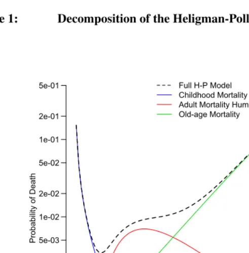
The eight parameters of the Heligman-Pollard model control three separate additive components corresponding to three age ranges of the mortality schedule (child mortality, young adult mortality, and late life mortality), and each parameter has a demographic interpretation (Heligman and Pollard 1980; McNown and Rogers 1989; Rogers and Gard 1991). Figure 1 displays each of these components and the sum of all three, i.e. the
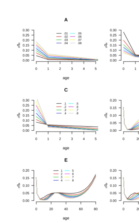
final curve.11 Table 1 provides interpretations for the parameters, and the eight panels of
Figure 2 illustrate the effects of each parameter individually. Each panel plots the modeled mortality schedule with variation in a single parameter while holding the others constant.
Table 1: Heligman-Pollard parameters
Parameter Description
A Level of child mortality, approximately the probability of dying
between ages 1 and 2,1q1
B Difference between age 0 and 1 mortality probabilities
C Decline in mortality during childhood
D Level (or height) of mortality hump
E Inversely related to the width of the mortality hump
F Location of the mortality hump on the age axis
G Late life mortality, intercept of Gompertz curve at age 0
H Late life mortality, slope of of Gompertz curve
11Figures 1 and 2 are plotted usingA= 0.06008,B= 0.31087,C= 0.34431,D= 0.00698,E= 1.98569,
F = 26.7107,G= 0.00022,H = 1.08800which correspond to the nearly 100nqxvalues in the Brass
The first three (A,B&C) control the first component and describe early child
mor-tality. A roughly approximates mortality at age one and can be taken as a measure of
the intensity or level of child mortality (McNown and Rogers 1989; Rogers and Gard
1991; Hartmann 1987).B is the age displacement variable (Rogers and Gard 1991) and
reflects the difference between mortality at ages 1 and 0. As the value ofB increases,
1q0 decreases below 0.5 and begins to approach1q1 (Rogers and Gard 1991). Finally,
Cindicates how quickly mortality decreases during childhood and into the young adult
years. ParametersA,B &Call have domain (0, 1). Declines inAare consistent with
decreasing child mortality (Hartmann 1987). Because of the potential direct impact of pediatric AIDS deaths and the indirect impact of adult AIDS mortality on child mortal-ity, we expect the level of child mortality to increase from period to period, leading to
increases inAfor both sexes as time goes on and the HIV epidemic grows.
Figure 1: Decomposition of the Heligman-Pollard model
0 20 40 60 80 100
5e-04 1e-03 2e-03 5e-03
1e-02
2e-02
5e-02
1e-01 2e-01
5e-01
Age (Years)
Pro
ba
bi
lit
y
of
D
ea
th
The second component of the model is designed to reproduce the ‘accident’ hump in many male mortality schedules, and possibly maternal mortality in female mortal-ity schedules (Heligman and Pollard 1980; Hartmann 1987; McNown and Rogers 1989; Rogers and Gard 1991). When it reflects accidents, the hump peaks in the (early) twen-ties. We reinterpret the hump to reflect AIDS mortality at young and slightly older adult
ages, so in our use the peak is older and taller. ParameterDcontrols the level or intensity
of young adult mortality,Eis inversely related to the spread of the hump, andF locates
its position along the age axis (Heligman and Pollard 1980; McNown and Rogers 1989;
Rogers and Gard 1991). ParametersDandEhave domains (0, 1) and (0,∞) respectively,
while the domain ofF is less clear. We restrictF to the domain (15, 55) because we do
not expect a large number of AIDS deaths at ages older than 55. With the hump reflect-ing AIDS mortality, we expect increasreflect-ing levels of adult mortality for both sexes as time
progresses, i.e. increases inD. As the epidemic matures we also expect a broadening and
aging of the adult mortality hump, i.e. decreases inEand increases inF. Note that if
Dis sufficiently small the other two parameters controlling this component of the curve
have no influence. Inspecting Equation 1 and the panel for parameterDin Figure 2, one
can see that the second component of the model is composed of the product ofDand the
effects ofEandF, so a smallDessentially negates the effect of the spread and location
parameters.
The last two parameters control the late life mortality section of the curve and describe
the steep increase in mortality at those ages.12 Parameter Gmeasures the base level of
mortality at these ages (x= 0) andHdefines the rate of increase (Rogers and Gard 1991).
ParametersGandH are the intercept and slope of the Gompertz curve respectively and
take domains (0, 1) and (0,∞) respectively.
The aim is to identify values for the eight parameters that produce a curve that matches a set of mortality measures at various ages. The set of eight parameter values is then the compact, interpretable description of mortality that we want, and the curve they represent is a smoothed version of the empirical data.
3.2 Data
We use data describing mortality and HIV prevalence. Mortality data come from the Ag-incourt health and demographic surveillance system (HDSS) site in South Africa (Kahn et al. 2007). The site is located in a rural area of Mpumalanga Province in the northeast of South Africa where HIV prevalence is a little less than 30% (Department of Health,
12Kotaski (1992) formulated a nine-parameter version of the HP with a Makeham functionK as the old-age term
Republic of South Africa 2006). Using time-sex-age-specific counts of deaths and person years for the period 1994-2007, we compute time-sex-age-specific probabilities of dying
(nqx) using standard life table methods. Our estimation procedure requires the
denomina-tor in the probability of dying (lx) to have approximately the same scale as the empirical
data.13 This requires us to rescale thelxcolumn of the life table, and we do this using MS
Excel’s ‘solver’ utility to find a value forl0that yields the same total number of person
yearsT0in the life table as there are in the observed data.
Because the annual data contain few deaths and are rather ‘noisy,’ we aggregate across time. Periods are chosen to contain years with similar mortality rates and to capture as much variability in the age pattern of mortality as possible. The four periods we use are:
1994-1997 (lmale
0 = 1,917,l
f emale
0 = 1,873), 1998-2001 (l
male
0 = 2,100,l
f emale
0 =
2,049), 2002-2004 (lmale
0 = 1,896,l
f emale
0 = 1,822) and 2005-2007 (l
male
0 = 1,974,
lf emale0 = 1,893). Figure 3 displays the aggregated and rescaled mortality schedules for males and females. Appendix A lists the data as used in our analysis and Appendix F details the process for aggregating into these periods.
Data describing the trend in HIV prevalence in Mpumalanga Province are taken from reports published by the South African Department of Health (Department of Health, Re-public of South Africa 1995, 1996, 1997, 1998, 2003, 2006). For the most part these estimates are made using anonymous HIV test results from pregnant women who attend antenatal clinics. See section 3.4 for further description of this data source. Antiretro-viral therapy became available in this population starting in 2007, and as of this writing coverage is still not complete (Gomez-Olive et al. 2013).
13We do not know the actual number of people left alive at each age,l
x, but we need to approximate it closely
Figure 2: Variation plots for the Heligman-Pollard mortality model
0 1 2 3 4 5
0.00 0.05 0.10 0.15 0.20 0.25 0.30 A age n qx .01 .02 .03 .04 .05 .06 .07 .08
0 1 2 3 4 5
0.00 0.05 0.10 0.15 0.20 0.25 0.30 B age n qx .1 .2 .3 .4 .5 .6 .7 .8
0 1 2 3 4 5
0.00 0.05 0.10 0.15 0.20 0.25 0.30 C age n qx .1 .2 .3 .4 .5 .6 .7 .8
0 20 40 60 80
0.00 0.05 0.10 0.15 0.20 D age n qx .01 .02 .03 .04 .05 .06 .07 .08
0 20 40 60 80
0.00 0.05 0.10 0.15 0.20 E age n qx 1 2 3 4 5 6 7 8
0 20 40 60 80
0.00 0.05 0.10 0.15 0.20 F age n qx 15 20 25 30 35 40 45 50
0 20 40 60 80
0.00 0.05 0.10 0.15 0.20 0.25 0.30 G age n qx .0001 .0002 .0003 .0004 .0005 .0006 .0007 .0008
0 20 40 60 80
0.00 0.05 0.10 0.15 0.20 0.25 0.30 H age n qx 1.05 1.06 1.07 1.08 1.09 1.10 1.11 1.12
Notes: nqxrefers to the probability of death in the intervalxtox+n. Each panel plots the age-specific
probabilities of death when varying a single parameter value in the HP model while holding all others
Figure 3: Age pattern of the probability of dying, Agincourt 1994-2007
●●
● ● ● ● ● ●
● ●
● ●
● ●
● ●
● ●
● ●
●
0.0 0.1 0.2 0.3 0.4 0.5 0.6
Male
age
n
qx
0 5 15 25 35 45 55 65 75 85
●94−97
98−01 02−04 05−07
●●
● ● ● ● ● ● ● ● ● ● ●
●
● ●
● ●
●
●
0.0 0.1 0.2 0.3 0.4 0.5 0.6
Female
age
n
qx
0 5 15 25 35 45 55 65 75 85
●94−97
98−01 02−04 05−07
Notes: nqxrefers to the probability of death in the intervalxtox+n
3.3 Bayesian melding estimation
We now turn to the Bayesian method used for parameter estimation. Bayesian melding searches the joint parameter space for sets of parameter values that are most likely given the data and what we know beforehand about the typical values for the parameters and the age patterns of mortality that we are modeling. Instead of identifying just the one most likely set of parameter values, it finds the most likely region of the parameter space and returns the sets of parameter values in that region. Each set of parameter values is associated with a probability corresponding to how well it reflects the data. These probabilities are used to construct joint distributions of the parameter values, which allow us to draw inferences about and characterize uncertainty around the parameter estimates themselves and the mortality patterns they represent.
The following discussion of Bayesian melding is adapted from Clark, Thomas, and Bao (2012). For a detailed discussion of Bayesian Melding see Poole and Raftery (2000). In the Bayesian framework parameters are treated as random variables. Prior beliefs about
the parameters are quantified in the form of a joint probability densityp(θ), whereθ is
a vector of parameters for which we will make inference. The datayare brought in by
specifying a likelihoodL(y|θ), which is the probability of the observed data for a given
dy-ing in each time-sex-age cell. We use the binomial likelihood because the observednqx
are probabilities describing a binary outcome (see appendix G for a full specification of the likelihood). Bayesian melding (Poole and Raftery 2000) is designed for problems in which a deterministic model – such as the Heligman-Pollard mortality model – is used in
the likelihood function. LetM represent the model which transforms a set of parameter
inputsθinto a set of model outputsφ =M(θ). The prior density for the model inputs
p(θ)and a likelihood for the outputs and the dataL(M(θ))are combined to produce the
posterior distribution for the model inputs. Using Bayes’ Theorem and the marginal
den-sity of the datap(y), we can update our prior beliefs to obtain the posterior distribution14
p(θ|y)∝ L(y|M(θ))p(θ) (2)
which is used to make inference forθ.
In our analysis of the Heligman-Pollald mortality model, we specify independent uni-form priors that are intended to be fairly uninuni-formative, placing most of the influence with the observed data. With these priors, our aim is to exert as little influence as possible on the parameter outputs while keeping the parameter output values in plausible ranges. The prior distributions are:
A∼U[0,0.25] D∼U[0,0.25] G∼U[0,0.01]
B∼U[0,1] E∼U[0,20] H ∼U[1,1.5]
C∼U[0,1] F ∼U[15,55].
Inference is performed by sampling fromp(θ|y)and summarizing the resulting
pos-terior sample. We can evaluate the model for each set of inputs in the pospos-terior sample
to obtain a posterior sample of the model outputsp(φ|y). Note that the posterior sample
reflects the distribution of model outputs, and thus the quantiles of the posterior sample
can be used to make probabilistic statements about the values of the model outputs (qx).
In this analysis, we use the Incremental Importance Sampling Algorithm (see ap-pendix H for a discussion of IMIS) to sample 400 sets of parameter values in the final resample from the posterior distribution, which can then be used to calculate 400 separate
nqxschedules, each covering the whole age range. The result is an approximation of the
posterior distribution ofnqx values, i.e. a distribution of the probabilities of dying,not
the number of deaths, which is what we used in the likelihood, and therefore what we want. To produce a predicted distribution of the number of deaths that we can compare
14Equation 2 arises from the fact that the marginal density of the data,p(y), does not depend onθ, so the
to the data, we simulate death counts from the posterior distribution ofnqxvalues. This
is accomplished using the binomial distribution with the observed number of people at
risk of dying and annqxvalue sampled at random from the posterior distribution ofnqx.
The number of deaths is then divided by the number of people at risk of dying to produce
a predictednqxvalue. This procedure is repeated many times to yield a distribution of
predictednqxvalues. Figure 4 plots thenqxvalues simulated from the posterior output
distribution for the first (flat hump) and the last (more intense and concentrated hump)
periods for males. The gray clouds are the simulatednqxvalues. This figure shows how
the simulated, predictednqxvalues cluster around the observed age-specific death
proba-bilities and that this model can closely fitnqxschedules at the beginning and peak of the
HIV epidemic. Appendix D presents the prior and posterior densities for each parameter by sex and year.
Figure 4: Predictive distributions of male age-specific probabilities of dying
for flat hump (’94-97) and intense hump (’05-07) periods
0 20 40 60 80 100
0.0 0.2 0.4 0.6 0.8
age
n
qx
●●
● ● ● ● ● ●
● ●
● ●
● ●
● ●
● ●
● ●
● ●
Male 1994−1997 Observed Median 95% CI 50% CI
Posterior Predictive Samplei of 400
0 20 40 60 80 100
0.0 0.2 0.4 0.6 0.8
age
n
qx
● ●
● ● ● ●
● ●
● ● ●
● ●
● ●
● ●
● ●
● ● ●
Male 2005−2007 Observed Median 95% CI 50% CI
Posterior Predictive Samplei of 400
Notes: nqxrefers to the probability of death in the intervalxtox+n
Dellapor-tas, Smith, and Stavropoulos (2001) use a different Bayesian approach and report that the over-parameterization issue is usually resolved by using informative priors (Congdon
1993). Even with our relativelyuninformativepriors, the Bayesian approach solves this
problem. One way to assess over-parameterization is to examine the correlation between parameters. We present pairs plots for each sex/year combination in Appendix C. The
parameters are essentially uncorrelated exceptGandH, and the correlation ofGandH
is expected since they act together as a product.
Another difficulty in estimating the Heligman-Pollard model occurs when adult mor-tality is somewhat flat and the estimated hump parameters can take values beyond a plau-sible range (Rogers and Gard 1991; Hartmann 1987; Heligman and Pollard 1980). In
this case, the level parameterDmay be large and the location parameterFon order 100,
essentially creating a very broad, flat hump whose upswing merges into the natural rise in mortality at older ages. Fixing one or more parameters and estimating the others tends to resolve this problem (Congdon 1993; Rogers and Gard 1991; Hartmann 1987). Instead,
we let all the parameters vary simultaneously while restricting the range on parameterF
to between 15 and 55, which keeps the hump parameters in plausible ranges and prevents the hump from merging into old-age mortality.
3.4 Relationship between parameters and HIV prevalence over time
We investigate the temporal relationship between trends in the values of the Heligman-Pollard parameters and HIV prevalence. For each sex we plot the median value of the
parameter distributions for parametersA,D,E andF by the mean HIV prevalence in
Mpumalanga Province with a five-year lag (Figure 11). We expect increases in HIV prevalence to be followed by increases in both child and adult mortality, so there should be a positive relationship between both child and adult mortality and the level parameters
AandD. Additionally we expect the spread and location parametersEandF to reveal
changes in the general age structure of adult mortality affected by HIV. Table 4 presents the mean HIV prevalence levels for the relevant five-year lagged periods.
3.5 Calculating uncertainty around life table columns
An advantage of the Bayesian approach is the ability to estimate uncertainty bounds
around both the model parameters and theoutputs. Following a similar method advanced
by Lynch and Brown (2005), we exploit this to generate uncertainty bounds around the
other columns of a standard life table, in particular around the life expectancy,ex,
For each period and sex, the predictivenqxdistributions (see Appendix B) contain
400 individualnqxschedules from which we calculate a ‘distribution’ of 400 individual
life tables. We present the medianexdistributions in Figures 12 and Appendix C and the
mediane0ande10with measures of uncertainty summarized from their distributions in
Tables 4 and 6. We use these to make statistically valid statements about changes in the expectation of life.
4.
Results
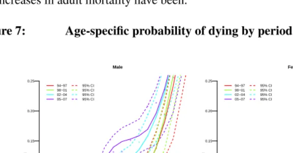
Figure 7 displays the period-specific fits, each period in a different color. For each period the light-colored dots in the background are the observed data, the solid lines are the median fitted curves, and the dashed lines define the 95% credible interval around the median, which are not required to be symmetric. The radical increases in age-specific mortality are obvious: massive increases for infants and very young children and for adults aged roughly 15-65. The increases are not uniform with age and peak for men in the early 40s and for women slightly younger. The corresponding decreases in life expectancy are listed in Table 4: men lost fifteen years of life expectancy, and women lost fourteen. The substantive objective of this work is to decompose these changes into their
constituent parts and relate those parts to changes in HIV prevalence.15
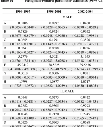
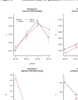
Table 5 presents the median parameter estimates and 95% credible intervals. Figure
8 plots the estimated values of parametersA,D,EandF over the four periods in our
study. The vertical dashed lines in this figure are the credible intervals around each point estimate.
4.1 Goodness of fit
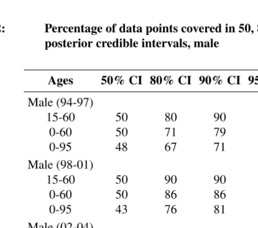
Before discussing the parameters themselves, we assess goodness of fit by calculating the percentage of data points contained within posterior credible intervals of varying lengths. Tables 2 and 3 contain the percentage of data points contained in the 50, 80, 90, 95, and 99 percent posterior credible intervals in three age ranges: 15-60 (adult mortality), 0-60 for males, and 0-95 for females. For each CI we should expect about the same percentage of data points to be contained within the interval. For virtually all years and both sexes, all of the data points in the adult ages are contained within the 99% CI with roughly 90 percent of data points in this age range in the 90 and 95% CIs. Adding in the childhood ages (rows labeled ‘0-60’) and oldest ages (rows labeled ‘0-95’) we see the model again does a good job of fitting these data for both sexes and all periods.
Numerous other parametric forms for the shape of human mortality have been pro-posed (Gage and Mode 1993; Wood et al. 2001), so in addition to showing how well the Heligman-Pollard model fits these data, we might also wish to know how well the HP model fits compared to other well-known parametric forms. We fit the four periods for both sexes with two other parametric models (using maximum likelihood), Gompertz-Makeham (Gompertz 1825; Gompertz-Makeham 1860) and Siler (Siler 1979, 1983), and show those fits with the median HP fit. Figures 5 and 6 plot these fits for all four periods. These plots make clear that the HP is able to best replicate all-age mortality in the presence of high HIV prevalence. During the first two periods when mortality is relatively flat in the adult years, all models do relatively well, but when the AIDS hump begins to grow, the other models do not have have the flexibility of the HP model with its three parameters govern-ing the adult hump, and consequently they miss the hump altogether.
Table 2: Percentage of data points covered in 50, 80, 90, 95 and 99%
posterior credible intervals, male
Ages 50% CI 80% CI 90% CI 95% CI 99% CI
Male (94-97)
15-60 50 80 90 90 100
0-60 50 71 79 86 100
0-95 48 67 71 86 100
Male (98-01)
15-60 50 90 90 90 100
0-60 50 86 86 86 100
0-95 43 76 81 81 90
Male (02-04)
15-60 60 90 90 90 100
0-60 57 86 86 86 93
0-95 48 71 81 81 86
Male (05-07)
15-60 50 80 90 90 100
0-60 50 79 86 86 100
Figure 5: Median HP fit and maximum likelihood fit for Gompertz-Makeham and Siler models to Agincourt data: Female
Figure 6: Median HP fit and maximum likelihood fit for Gompertz-Makeham and Siler models to Agincourt data: Male
Table 3: Percentage of data points covered in 50, 80, 90, 95 and 99% posterior credible intervals, female
Ages 50% CI 80% CI 90% CI 95% CI 99% CI
Female (94-97)
15-60 40 90 90 90 90
0-60 36 93 93 93 93
0-95 33 76 81 81 81
Female (98-01)
15-60 50 70 100 100 100
0-60 43 57 93 100 100
0-95 38 48 76 81 90
Female (02-04)
15-60 60 90 90 90 100
0-60 50 86 93 93 100
0-95 48 81 86 90 100
Female (05-07)
15-60 50 60 80 90 100
0-60 50 64 86 93 100
0-95 52 76 90 95 100
4.2 Child mortality
The increase in child mortality during the period when the HIV epidemic grows is
re-flected by increases in parameterAwhich is roughly the probability of dying between
ages one and two,1q1. The upper-left panel of Figure 8 displays a clearly upward trend in
the value of parameterAfor both male and female children. A quick visual comparison
of the credible ranges (dashed vertical line in Figure 8) reveals unambiguous increases in
parameterAduring the first two intervals and a possible decrease during the last interval.
4.3 Adult mortality
ParametersD,E,F,GandH control adult mortality. We focus onD,EandF because
they control the hump whileGandHdefine underlying adult mortality. The plots in
Fig-ure 8 reveal striking changes in the hump parameters (upper right and lower two panels).
during the first interval for males with little to no overlap in the credible intervals from one period to the next. Figures 9 and 10 plot the period-sex-specific hump component of the model in isolation without the other components of the mortality schedule. Figure 9 plots the hump for each sex by period and clearly reveals the growth in the hump from period to period. Figure 10 displays the hump curves with the male and female humps in a single plot for each period, so that the sexes can be compared easily. This figure confirms that although men appear to have slightly higher humps in all periods, the differ-ences between the sexes are small and insignificant except for the last period when women
have a substantially lower hump. These movements in parameterDrelate directly to the
growth of the mortality bulge observed for adults, and the highly regular and significant changes (i.e. non-overlapping credible intervals) demonstrate how large and important the increases in adult mortality have been.
Figure 7: Age-specific probability of dying by period for Agincourt
0.00 0.05 0.10 0.15 0.20 0.25
Male
age
0 5 15 25 35 45 55 65 75 85
n
qx 94−97 98−01 02−04 05−07
95% CI 95% CI 95% CI 95% CI
0.00 0.05 0.10 0.15 0.20 0.25
Female
age
0 5 15 25 35 45 55 65 75 85
n
qx 94−97 98−01 02−04 05−07
95% CI 95% CI 95% CI 95% CI
Notes: Median fitted curves (solid lines) with 95% credible intervals (dashed lines). Observednqxvalues in
light-colored dots.nqxrefers to the probability of death in the intervalxtox+n.
Trends in the width parameterE(inversely related to the width of the hump) indicate
Changes in the location parameterF(location of the hump on the age axis) reveal that the hump has steadily become older for women and became younger and then older again for men. Figures 8 and 10 suggest that the hump is typically slightly older for males; i.e. the male humps usually peak at slightly older ages regardless of the height or spread of the hump. This is especially pronounced during the first period when the mortality effects of HIV are first being observed. Recall that women tend to be infected with HIV at younger ages compared to men and thus have high mortality at younger ages. The location param-eter accurately reflects this previously observed pattern with the male median estimate
ofFconsistently outpacing the female estimate. Women experience increasing mortality
during their 30s (reflecting a female incidence profile that starts infecting a significant number of women in their early 20s), while for men the hump grows from the late 30s to the mid 40s. The unusually large value of the location parameter in the first period for men probably results from a small increase in mortality around the late 40s to early 50s. Because this is the first period, it is unlikely that this small hump is a result of HIV-related deaths. Rather, HIV probably begins to affect the male mortality schedule between the first and second periods, at which time the location and level parameters begin to pick up increasing male mortality in the late 30s, consistent with previously observed HIV mor-tality patterns. Changes in the hump for men are seen best in Figure 9; clearly between the first and second periods the male hump increases slightly in intensity and shifts back to the expected age range.
Table 4: Life expectancy for Agincourt and HIV prevalence for
Mpumalanga Province
Period Male e0a ∆Maleb Female e0a ∆FemalebPrev.c ∆Pd Prev. Period
1994-1997 67.3 — 73.5 1.3 — 1990-1992
(65.2 – 72.0) (72.0 – 74.9)
1998-2001 63.0 -4.3 69.7 -3.8 11.6 10.4 1993-1996
(61.3 – 65.4) (67.8 – 71.8)
2002-2004 53.5 -9.5 59.7 -10.0 26.6 15.0 1997-1999
(51.6 – 55.4) (58.1 – 61.9)
2005-2007 52.2 -1.4 59.4 -0.4 29.2 2.5 2000-2002
(50.6 – 54.4) (56.4 – 64.8)
Total Change: -15.2 -14.2 27.9
a e
0in years. 95% credible intervals for e0in parentheses. b∆(Male, Female) is change in median e
0from previous period.
c HIV prevalence is for the surrounding province (Mpumalanga) for all ages in the period roughly five years before the
period in whiche0is estimated. Source for prevalence estimates: Department of Health, Republic of South Africa
(Department of Health, Republic of South Africa 1995, 1996, 1997, 1998, 2003, 2006).
Table 5: Heligman-Pollard parameter estimates (95% CI)
1994-1997 1998-2001 2002-2004 2005-2007
MALE
A 0.0106 0.0297 0.0460 0.0262
( 0.0059 - 0.0148 ) ( 0.0228 - 0.0365 ) ( 0.0390 - 0.0529 ) ( 0.0194 - 0.0321 )
B 0.7829 0.9724 0.9652 0.7754
( 0.6673 - 0.8979 ) ( 0.9248 - 0.9980 ) ( 0.8928 - 0.9981 ) ( 0.6930 - 0.8609 )
C 0.0855 0.1791 0.3526 0.2083
( 0.0320 - 0.1501 ) ( 0.1149 - 0.2336 ) ( 0.2801 - 0.4191 ) ( 0.1573 - 0.2589 )
D 0.0243 0.0388 0.0726 0.1199
( 0.0160 - 0.0327 ) ( 0.0324 - 0.0445 ) ( 0.0618 - 0.0836 ) ( 0.1062 - 0.1338 )
E 5.2779 4.5021 3.1653 3.7761
( 3.4764 - 7.1116 ) ( 3.0783 - 5.6768 ) ( 1.5618 - 4.6151 ) ( 2.9309 - 4.6871 )
F 45.2412 38.5225 39.5636 42.2610
( 41.4002 - 49.0394 ) ( 36.3215 - 40.5921 ) ( 35.6854 - 43.7599 ) ( 39.0647 - 44.7113 )
G 0.0010 0.0006 0.0021 0.0009
( 0.0003 - 0.0017 ) ( 0.0003 - 0.0009 ) ( 0.0010 - 0.0034 ) ( 0.0004 - 0.0015 )
H 1.0798 1.0877 1.0717 1.0827
( 1.0725 - 1.0872 ) ( 1.0822 - 1.0939 ) ( 1.0630 - 1.0805 ) ( 1.0772 - 1.0887 )
FEMALE
A 0.0148 0.0275 0.0422 0.0356
( 0.0118 - 0.0181 ) ( 0.0227 - 0.0334 ) ( 0.0382 - 0.0473 ) ( 0.0305 - 0.0417 )
B 0.7852 0.9305 0.9792 0.8563
( 0.7047 - 0.8732 ) ( 0.8589 - 0.9942 ) ( 0.9520 - 0.9985 ) ( 0.8085 - 0.9027 )
C 0.1048 0.2120 0.2245 0.2373
( 0.0697 - 0.1409 ) ( 0.1621 - 0.2568 ) ( 0.2065 - 0.2447 ) ( 0.2064 - 0.2669 )
D 0.0126 0.0303 0.0688 0.0867
( 0.0083 - 0.0167 ) ( 0.0266 - 0.0348 ) ( 0.0642 - 0.0733 ) ( 0.0808 - 0.0930 )
E 14.5269 2.6527 2.5174 2.5266
( 13.0611 - 15.8447 ) ( 1.9731 - 3.3408 ) ( 2.1914 - 2.8271 ) ( 2.0314 - 3.1009 )
F 31.1959 36.5381 38.1891 40.6617
( 28.1650 - 34.0361 ) ( 34.0823 - 39.2770 ) ( 37.0759 - 39.2378 ) ( 38.9361 - 42.2265 )
G 0.0003 0.0003 0.0001 0.0001
( 0.0002 - 0.0004 ) ( 0.0002 - 0.0004 ) ( 0.0000 - 0.0001 ) ( 0.0000 - 0.0002 )
H 1.0958 1.0900 1.1110 1.1092
Figure 8: Estimated values for parametersA, D, E, F by sex and time
M
M
M
M
0.01 0.02 0.03 0.04 0.05
Parameter A (Level of Child Mortality)
period
A
94−97 98−01 02−04 05−07
F
F
F
F
M
F
Male Female
95% CI 95% CI
M
M
M
M
0.02 0.04 0.06 0.08 0.10 0.12
Parameter D (Level of Adult Mortality)
period
D
94−97 98−01 02−04 05−07
F
F
F
F
M
M
M M
2 4 6 8 10 12 14 16
Parameter E (Spread of Mortality Hump)
period
E
94−97 98−01 02−04 05−07
F
F F F
M
M
M
M
30 35 40 45
Parameter F (Location of Mortality Hump)
period
F
94−97 98−01 02−04 05−07
F
F
F
Figure 9: Hump component for all periods and both sexes
20 40 60 80
−8 −6 −4 −2 0
Male
age
log(
n
qx
)
94−97 98−01 02−04 05−07
95% CI 95% CI 95% CI 95% CI
20 40 60 80
−8 −6 −4 −2 0
Female
age
log(
n
qx
)
94−97 98−01 02−04 05−07
95% CI 95% CI 95% CI 95% CI
Comparing humps from the last two periods with those from the first two, two things
are clear: 1) the hump becomes taller reflecting the increases in the level parameter,D,
and 2) the humps broaden as the width parameter, E, decreases. The widening of the
humps is asymmetric with the bulk of the changes happening at older ages (35+) where the hump appears to flatten out. These changes reflect the spreading of increased adult mortality into the older middle adult ages, 35-45, likely reflecting a widening of the age profile of incidence resulting in deaths associated with HIV at increasingly older ages.
4.4 HIV prevalence
Figure 11 displays the median parameter values forA,D,E andF along with the
Figure 10: Hump component for each sex for each period
20 40 60 80
−8 −7 −6 −5 −4 −3 −2 −1
1994−1997
age
log(
n
qx
)
Male Female
95% CI 95% CI
20 40 60 80
−8 −7 −6 −5 −4 −3 −2 −1
1998−2001
age
log(
n
qx
)
20 40 60 80
−8 −7 −6 −5 −4 −3 −2 −1
2002−2004
age
log(
n
qx
)
20 40 60 80
−8 −7 −6 −5 −4 −3 −2 −1
2005−2007
age
log(
n
qx
Figure 11: Selected parameter values by 5-year lagged HIV prevalence
●
●
●
●
0 5 10 15 20 25 30
0.00 0.01 0.02 0.03 0.04
Male − A (Level of Child Mortality)
HIV Prevalence A 94−97 98−01 02−04 05−07 ● ● ● ●
0 5 10 15 20 25 30
0.00 0.01 0.02 0.03 0.04
Female − A (Level of Child Mortality)
HIV Prevalence A 94−97 98−01 02−04 05−07 ● ● ● ●
0 5 10 15 20 25 30
0.02 0.04 0.06 0.08 0.10 0.12
Male − D (Level of Adult Mortality)
HIV Prevalence D 94−97 98−01 02−04 05−07 ● ● ● ●
0 5 10 15 20 25 30
0.02 0.04 0.06 0.08 0.10 0.12
Female − D (Level of Adult Mortality)
HIV Prevalence D 94−97 98−01 02−04 05−07 ● ● ● ●
0 5 10 15 20 25 30
2 4 6 8 10 12 14
Male − E (Spread of Mortality Hump)
HIV Prevalence E 94−97 98−01 02−04 05−07 ● ● ● ●
0 5 10 15 20 25 30
2 4 6 8 10 12 14
Female − E (Spread of Mortality Hump)
HIV Prevalence E 94−97 98−01 02−04 05−07 ● ● ● ●
0 5 10 15 20 25 30
32 34 36 38 40 42 44
Male − F (Location of Mortality Hump)
HIV Prevalence F 94−97 98−01 02−04 05−07 ● ● ● ●
0 5 10 15 20 25 30
32 34 36 38 40 42 44
Female − F (Location of Mortality Hump)
HIV Prevalence
F
94−97
98−01 02−04
05−07
For all periods and both sexes, the level parametersAandDincrease with HIV
preva-lence, except forAduring the final period. During the final interval the overall level of
child mortality is reduced, perhaps reflecting the success of programs to limit mother-to-child transmission (for a brief review see Doherty, McCoy, and Donohue 2005). The largest increase in level is in the second interval (between the second and third periods) for women, coming just after the largest increase in prevalence; the largest increase for men occurs in the last interval after ten years at high prevalence.
For parametersE(spread or width of hump) andF(location of hump) the relationship
with earlier prevalence is less neat but still regular and in-line with expectations. For both
sexes there is a downward slope to the relationship betweenE(width of the hump) and
earlier prevalence, indicating that as prevalence increases the hump becomes gradually wider; this is especially the case for women whose hump starts off much narrower than men’s.
For men the location of the hump moves from∼45to∼38and then back up to∼42.
In contrast, women have experienced a consistent ‘aging’ of the hump moving from∼31
to∼40. This indicates the agelocusof the mortality impact of HIV for men has hovered
at a little below age 40, while for women it has moved steadily to older ages and is now at about the same age as men.
4.5 Life expectancy
Table 6 reports expectation of life at birth and age ten for the four periods for both sexes, and Figure 12 plots the median expectation of life schedule with 95% credible intervals. There was a precipitous decline in life expectancy over the entire period with the largest drops occurring between the second and third periods for both sexes. At the beginning of observation during 1994-1997 a male infant could expect to live 67.3 years, and a female infant 73.5. By the end of the final period, a male infant expected only 52.2 years and a female 59.4. Men lost 15.2 years of life expectancy, and women lost 14.2. Judging from the credible intervals, change over the whole period is very significant, with the bulk of the significant drop between periods two and three.
The expectation of life at age ten is not affected by child mortality and consequently describes adult mortality more clearly. Table 6 shows clearly that the majority of the changes in the expectation of life at birth result from changes in adult mortality; the
changes ine10closely track, and in the most recent period, exceed the changes ine0. The
in mortality at about the turn of century, reflecting increases in HIV prevalence during the 1990s, see Table 4.
Table 6: Life expectancy at birth and age 10
Period e0a ∆e0b e10a ∆e10b
MALE
1994-1997 67.3 — 59.2 —
(65.2 – 72.0) (57.2 – 64.2)
1998-2001 63.0 -4.3 56.8 -2.5
(61.3 – 65.4) (55.0 – 59.4)
2002-2004 53.5 -9.5 47.9 -8.9
(51.6 – 55.4) (46.1 – 49.8)
2005-2007 52.2 -1.4 45.1 -2.7
(50.6 – 54.4) (43.8 – 47.4)
FEMALE
1994-1997 73.5 — 66.0 —
(72.0 – 74.9) (64.7 – 67.3)
1998-2001 69.7 -3.8 63.4 -2.6
(67.8 – 71.8) (61.8 – 65.6)
2002-2004 59.7 -10.0 54.5 -9.0
(58.1 – 61.9) (53.1 – 56.5)
2005-2007 59.4 -0.4 53.4 -1.0
(56.4 – 64.8) (50.4 – 59.0)
Total Change: -14.2 -12.6
a
exin years. 95% credible intervals for exin parentheses.
b
∆exis change in median exfrom previous period.
5.
Discussion
5.1 Summary
parameters of the Heligman-Pollard model describe the shape of the age-specific nqx
schedule in three age ranges. We estimate the model using the Bayesian melding method
with IMIS to produce robust estimates of the parameter values, thenqxschedules output
by the model, and the corresponding life tables in four periods during which the HIV epidemic grew rapidly in this population. The Bayesian framework yields probabilistic measures of uncertainty around all of these estimates, and we use these to compare both
parameter estimates andnqxvalues over time and between the sexes.
Figure 12: exschedule predictive distribution with median and 95% CI
0 20 40 60 80
age
0 10 20 30 40 50 60 70 80 90 100
ex
Female 94−97 98−01 02−04 05−07
95% CI 95% CI 95% CI 95% CI
0 20 40 60 80
age
0 10 20 30 40 50 60 70 80 90 100
ex
Male 94−97 98−01 02−04 05−07
95% CI 95% CI 95% CI 95% CI
Notes: Observed data are represented as lightly colored dots.
The evidence from Agincourt demonstrates the profound effects of HIV on mortality. With a lag of several years after increases in HIV prevalence of 10-15%, the mortality of young children and adults increased dramatically. The corresponding drops in the expectation of life at birth removed about 15 years of life from the average person living in the Agincourt area. All of these changes are highly unlikely to have occurred by chance. Although this is not a new finding, we contribute an unusual nuance – the sex-specific age pattern of increases in mortality following increases in HIV prevalence succinctly summarized with an elegant parametric model.
in a temporal sequence consistent with changes in HIV prevalence. The increases in
young child mortality are captured with parameterA, and the appearance and growth of
the hump in adult mortality are reflected by changes in the ‘hump parameters’ –D,Eand
F. The hump level parameter progressively increases, and the hump spread parameter
decreases, corresponding to a gradual widening of the hump. Sex differences in these dy-namics suggest that the epidemic started and stays slightly older for men, and for women the epidemic started in a very narrow, young age range and gradually expanded to in-clude older ages. The estimated parameters succeed as a parsimonious and informative description of the age-specific changes in mortality as the HIV epidemic grew.
The Bayesian melding estimation procedure allows us to make robust fits of the eight-parameter Heligman-Pollard model of age-specific mortality to period-sex-age-specific mortality rates covering four phases of the growing HIV epidemic in the Agincourt study population. This Bayesian technique also allows us to characterize uncertainty in both the parameters and outputs of the model (the estimated mortality age schedule) without assuming any special properties for or relationships among the parameters. Bayesian melding results in a joint posterior distribution of the parameters. Running this
poste-rior through the model yields a posteposte-rior distribution ofnqxschedules from which counts
of deaths can be simulated and transformed into predictednqx schedules, from which
predicted life tables can be constructed. This results in a distribution of life tables, or equivalently, a predictive distribution for each column in the life table from which we cal-culate measures of uncertainty. The resulting estimates and credible intervals allow us to make strong probability-based statements about differences between mortality schedules and components of mortality schedules.
5.2 R package
We have released anR package,HPbayes(Sharrow 2011) that implements all of the
methods described in this paper, and we will continue to develop and improve that
pack-age. The package is available as a standardRpackage from CRAN that can be run using
the R statistical software. The user supplies age-specific counts of deaths and person
6.
Acknowledgements
This project was supported by grants K01 HD057246, R01 HD054511 and R01 HD070936 from the Eunice Kennedy Shriver National Institute of Child Health and Human Develop-ment (NICHD) of the National Institutes of Health (NIH), USA. The content of this work is solely the responsibility of the authors and does not necessarily represent the official views of the the NIH. Without the Agincourt HDSS site in South Africa this work would not have been possible; we thank the respondents, field staff and management of the site for sharing their valuable data and time with us. Thanks are due to key funding partners of the Agincourt site who have enabled the ongoing work of the MRC/Wits University Agincourt Unit: the Anglo-American ChairmanŠs Fund, The Andrew W. Mellon Founda-tion, The William and Flora Hewlett FoundaFounda-tion, the National Institutes of Health (NIH) grant number R24 AG032112 and the Wellcome Trust grant numbers 058893/Z/99/A and 069683/Z/02/Z. Finally, we are especially grateful to Jason Thomas, Le Bao, Adrian Raftery and members of the BayesPop working group at the University ofWashington for
their discussion, comments and assistance with various aspects of this work ˝U in
References
Adjuik, M., Smith, T., Clark, S.J., Todd, J., Garrib, A., Kinfu, J., Kahn, K., Mola, M., Ashraf, A., Masanja, H., Adazu, K., Sacarlal, J., Alam, N., Marra, A., Gbangou, A., Mwageni, E., and Binka, F. (2006). Cause-specifc mortality rates in sub-Saharan
Africa and Bangladesh. Bulletin of the World Health Organization 84(3): 181–188.
doi:10.2471/BLT.05.026492.
Alkema, L., Raftery, A.E., and Clark, S.J. (2007). Probabilistic projections of HIV
prevalence using Bayesian melding. The Annals of Applied Statistics1(1): 229–248.
doi:10.1214/07-AOAS111.
Bebbington, M., Lai, C.D., and Zitikis, R. (2007). Modeling human mortality using
mixtures of bathtub shaped failure distributions.Journal of Theoretical Biology245(3):
528–538.doi:10.1016/j.jtbi.2006.11.011.
Blacker, J. (2004). The impact of AIDS on adult mortality: evidence from national and
regional statistics.AIDS18(2): 19–26. doi:/10.1097/00002030-200406002-00003.
Botha, J.L. and Bradshaw, D. (1985). African vital statistics - a black hole?South African
Medical Journal67: 977–981.
Carriere, J.F. (1992). Parametric models for life tables. Insurance: Mathematics and
Economics Insurance: Mathematics and Economics14(1): 77–100.
Clark, S.J. (2002). INDEPTH Mortality Patterns for Africa. In: INDEPTH NETWORK
(ed.)Population, Health, and Survival at INDEPTH Sites. IDRC: 83–128, vol. 1.
Congdon, P. (1993). Statistical graduation in local demographic analysis and projection.
Journal of the Royal Statistical Society. Series A (Statistics in Society)156(2): 237–
270.
Crum, N.F., Riffenburgh, R.H., Wegner, S., Agan, B.K., Tasker, S.A., Spooner, K.M., Armstrong, A.W., Fraser, S., Wallace, M.R., and Triservice AIDS Clinical Consor-tium (2006). Comparisons of causes of death and mortality rates among HIV-infected persons: analysis of the pre-, early, and late HAART (highly active antiretroviral
therapy) eras. Journal of Acquired Immune Deficiency Syndromes 41(2): 194–200.
doi:/10.1097/01.qai.0000179459.31562.16.
Dabis, F. and Ekpini, E.R. (2002). HIV-1/AIDS and maternal and child health in Africa.
Lancet359(9323): 2097–2104.doi:/10.1016/S0140-6736(02)08909-2.
in resource poor countries - translating research into policy and practice.Journal of the
American Medical Association283: 1175–1182.
Debón, A., Montes, F., and Sala, R. (2005). A comparison of parametric models for mortality graduation: Application to mortality data for the Valencia region (Spain).
SORT29(2): 269–288. doi:/10.1111/j.1751-5823.2006.tb00171.x.
Dellaportas, P., Smith, A.F.M., and Stavropoulos, P. (2001). Bayesian analysis of
mor-tality data. Journal of the Royal Statistical Society: Series A 164(2): 275–291.
doi:/10.1111/1467-985X.00202.
Department of Health, Republic of South Africa (1995). Fifth national HIV survey in women attending antenatal clinics of the public health services in South Africa, Octo-ber/November. Republic of South Africa: Department of Health.
Department of Health, Republic of South Africa (1996). Sixth national HIV survey of women attending antenatal clinics of the public health services in the republic of South Africa, October/November 1995. Republic of South Africa: Department of Health.
Department of Health, Republic of South Africa (1997). Seventh national HIV survey of women attending antenatal clinics of the public health services, October/November 1996. Republic of South Africa: Department of Health.
Department of Health, Republic of South Africa (1998). Eighth annual national HIV sero-prevalence survey of women attending antenatal clinics in South Africa, 1997. Republic of South Africa: Department of Health.
Department of Health, Republic of South Africa (2003). National HIV and syphilis ante-natal sero-prevalence survey in South Africa: 2002. Republic of South Africa: Depart-ment of Health.
Department of Health, Republic of South Africa (2006). National HIV and syphilis ante-natal sero-prevalence survey in South Africa: 2005. Republic of South Africa: Depart-ment of Health.
Doherty, T.M., McCoy, D., and Donohue, S. (2005). Health system constraints to optimal coverage of the prevention of mother-to-child HIV transmission programme in South
Africa: lessons from the implementation of the national pilot programme. African
Health Sciences5(3): 213–218.doi:/10.1111/1467-985X.00202.
Dorrington, R., Bourne, D., Bradshaw, D., Laubscher, R., and Timaeus, L.M. (2001). The impact of HIV/AIDS on adult mortality in South Africa. South Africa: Burden of Disease Research Unit, Medical Research Council.
Trans-actions of the Faculty of Actuaries40: 98–134.
Foster, G. and Williamson, J. (2000). A review of current literature of the impact of
HIV/AIDS on children in sub-Saharan Africa.AIDS14(3): 275–284.
Gage, T.B. and Mode, C.J. (1993). Some laws of mortality: how well do they fit? Human
biology and an international record of research65(3): 445–461.
Gomez-Olive, F.X., Angotti, N., Houle, B., Klipstein-Grobusch, K., Kabudula, C.,
Menken, J., Williams, J., Tollman, S., and Clark, S.J. (2013). Prevalence of
HIV among those 15 and older in rural South Africa. AIDS Care 25(9): 1–7.
doi:/10.1080/09540121.2012.750710.
Gompertz, B. (1825). On the nature of the function expressive of the law of
hu-man mortality, and on a new mode of determining the value of life
contingen-cies. Philosophical Transactions of the Royal Society of London 115: 513–583.
doi:/10.1098/rstl.1825.0026.
Groenewald, P., Nannan, N., Bourne, D., Laubscher, R., and Bradshaw, D.
(2005). Identifying deaths from AIDS in South Africa. AIDS 19(2): 193–201.
doi:/10.1097/00002030-200501280-00012.
Hartmann, M. (1987). Past and recent attempts to model mortality at all ages. Journal of
Official Statistics3(1): 19–36.
Heligman, L. and Pollard, J.H. (1980). The age pattern of mortality. Journal of the
Institute of Actuaries107(1): 49–80.doi:/10.1017/S0020268100040257.
Hosegood, V., Vaenneste, A.M., and Timaeus, I.M. (2004). Levels and causes of
adult mortality in rural South Africa: the impact of AIDS. AIDS 18(4): 663–667.
doi:/10.1097/00002030-200403050-00011.
Jaffar, S., Grant, A.D., Whitworth, J., Smith, P.G., and Whittle, H. (2004). The natural
history of HIV-1 and HIV-2 infections in adults in Africa: a literature review.Bulletin
of the World Health Organization82(8): 462–469.
Kahn, K., Collinson, M.A., Gómez-Olivé, F.X., Mokoena, O., Twine, R., Mee, P.l., Afo-labi, S.A., Clark, B.D., Kabudula, C.W., and Khosa, A.e.a. (2012). Profile: Agincourt
health and socio-demographic surveillance system. International Journal of
Epidemi-ology41(4): 988–1001.doi:/10.1093/ije/dys115.
Kahn, K., Tollman, S.M., Collinson, M.A., Clark, S.J., Twine, R., Clark, B.D., Shabangu, M., Gomez-Olive, F.X., Mokoena, O., and Garenne, M.L. (2007). Research into health, population and social transitions in rural South Africa: Data and methods of the