Stabilization of linear systems of delay differential equations by the
delayed feedback method
Mohammad Mousa-Abadian
Department of Mathematics, Shahed University, P.O. Box 18151-159, Tehran, Iran.
E-mail: [email protected]
Sayed Hodjatollah Momeni-Masuleh∗ Department of Mathematics, Shahed University, P.O. Box 18151-159, Tehran, Iran.
E-mail: [email protected] Mohammad Haeri
Advanced Control Systems Lab, Electrical Engineering, Sharif University of Technology, Tehran, Iran.
E-mail: [email protected]
Abstract This paper consists of two folds. At first, we deal with the stability analysis of a linear system of delay differential equations. It is shown that the direct and cluster treatment methods are not applicable if there are some purely imaginary roots of the characteristic equation with multiplicity greater than one. To overcome the above difficulty, the system is decomposed into several subsystems. For the decomposition of a system, an invertible transformation is required to convert the matrices of the system into a block triangular (diagonal) form simultaneously. To achieve this goal, a necessary and sufficient condition is established. The second part concerns the stabilization of a linear system of delay differential equations using the delayed feedback method and design a controller for generating the desired response. More precisely, the unstable poles of the linear system of delay differential equations are moved to the left-half of the complex plane by the delayed feedback method. It is shown that the performance of the linear system of delay differential equations can be improved by applying the delayed feedback method.
Keywords. Linear time delay system, Stability analysis, Simultaneous block triangularization, Delayed
feedback method, Stabilization, Controller design.
2010 Mathematics Subject Classification. 93C30, 05C50, 93D15, 93D20.
1. Introduction
Linear system of delay differential equations (LSDDE) appears naturally in many branches of science and engineering. A common way of describing of an LSDDE is the state-space representation which is frequently used in control theory. Unlike ordinary differential equations (ODEs), in DDEs the rate of change of an unsteady process not only depends on the current state but also depends on its history state.
Received: 6 March 2018 ; Accepted: 2 March 2019.
∗Corresponding author.
The stability analysis of an LSDDE is extremely important from both theoretical and practical points of view [5, 15, 24]. Due to the presence of the delayed term in an LSDDE, the corresponding characteristic equation is a quasi-polynomial instead of a polynomial. Therefore, the stability analysis of such systems becomes more complicated. Rekasius [21], Walton and Marshall [26] and Olgac and Sipahi [17] presented some methods for the stability analysis of linear systems of DDEs. However, these methods cannot be applied for an arbitrary LSDDE. More precisely, Mesbahi and Haeri [14] presented an example of an LSDDE, which its characteristic equation has a multiple root with multiplicity greater than one, that the method proposed by Olgac and Sipahi cannot be used to analyze the stability of the system. They removed the repeated roots by decomposing the original 4 by 4 system into two subsystems with 2 by 2 dimension to perform the stability analysis of the original system.
One of the most common types of a DDE is the retarded one. In a retarded LSDDE, the derivative term ˙x, does not depend on the delay. In this paper, we present some retarded linear systems of DDEs that confirm the cluster treatment method [17] is not applicable to the system’s stability analysis. Furthermore, we show that the direct method [26] leads us to ambiguous results in detecting the number of unstable poles of the presented systems. Nevertheless, decomposing the original linear systems of DDEs into several subsystems enables one to handle the above difficulties. To decompose an LSDDE with a single delay and with two state matrices, we need to find an invertible transformation that simultaneously transforms both state matrices of the system into block triangular (diagonal) forms.
The simultaneous triangularization (diagonalization) of a set of matrices has at-tracted a great deal of attention recently because of applications in multidimensional systems [3], discrete time switching systems [7] and differential inclusions [16, 23]. The following two questions are crucial in simultaneous triangularization (diagonal-ization): 1- When two or more generally, a finite set of matrices can be transformed simultaneously into a block triangular (diagonal) form? 2- What kind of transforma-tions can put the matrices into a block triangular (diagonal) form simultaneously? To answer the first question, one of the most famous classical theorems is McCoy’s theorem [13] which states that the pair of matrices {A, B} is triangularizable if and only ifp(A, B)(AB−BA) is nilpotent for every noncommutative polynomialp.
It is easy to show that every set of commutative matrices can be simultaneously transformed into an upper triangular form, but the converse is not true [6, 20]. Lev-itzky [20] proved that every semigroup of nilpotent matrices is triangularizable. For a semigroup ofnbynmatrices, sayF, over a field that contains all the eigenvalues of the members ofF and whose characteristic is either zero or greater than n2, Radjavi [19] proved thatF is triangularizable if and only if trace is permutable onF. Uhlig [25] proved that the finest simultaneous block diagonalization of nonsingular pair of real symmetric matrices A and B contains k blocks of dimensions n1, n2, . . . , nk if and only if the real Jordan normal form ofA−1B consists kJordan blocks of dimensions
n1, n2, . . . , nk. Laffey [10] showed that for every n byn matrices A and B (n ≤5) with the property that for allλ: A3 =B3 = (A+λB)5 = 0, the pair of matrices
His algorithm answers the first and second question for non-block triangularization and uses Shemesh’s idea [22] to compute the invertible transformation. Kaczorek [8] proved that a set ofN real matrices{A1, A2, . . . , AN} is triangularizable if and only
if there exists a full column rank matrixJ ∈Rn×n such thatrank[J A
iJ] =rfor i= 1,2, . . . , N.
However, the presence of a time delay in a system can cause various complications, but it can be useful in some senses. Kwon et al. [9] obtained the state feedback track-ing controller by the delayed feedback method. They show that the performance of a system can be improved by the delayed feedback method and also disturbance at-tenuation and robustness against parameters variation can be modified. As we know, a time delay can be a source for instability of an LSDDE. Nevertheless, Abdallah et al. [1] showed that some oscillatory systems can be stabilized by the delayed feed-back method. Pyragas [18] applied the delayed feedback method to control chaos and also he employed this type of feedback to stabilize the unstable periodic orbits. Usually, one of the major goals in control theory is controlling an equilibrium solution or equivalently, the regulator problem. In fact, in a regulator problem, one needs to obtain an asymptotically stable steady state solution which attracts all nearby initial conditions. Dahms et al. [2] considered the extended time-delayed feedback method to control unstable steady states.
In this paper, we show that the block simultaneous triangularization of a finite set of square matrices is equivalent to the existence of a common invariant subspace for the matrices. In this direction, we prove a proposition which characterizes the invariant subspaces of a matrix by means of generalized eigenvectors [11]. Further-more, we present some linear systems of DDEs that their stability analysis cannot be investigated by the direct and the cluster treatment methods. Also, we show that an unstable LSDDE can be stabilized by the delayed feedback method. In addition, we adopt this feedback for putting the poles of an LSDDE in suitable coordinates to generate a desired response for the system. More precisely, by the delayed feedback method, the settling time of the system can be remarkably reduced.
The remaining of the paper is organized as follows. In section 2, we introduce some required mathematical details and problem statement. Stability analysis of the linear systems of DDEs using decomposition of the matrices of the system into a block triangular (diagonal) form is considered in section 3. In section 4, stabilization of an unstable LSDDE by the delayed feedback method is discussed. Section 5 is devoted to design a controller via the delayed feedback method. Finally, conclusion is available in section 6.
2. Mathematical details and problem statement
2.1. Definitions, lemmas and theorems. In this section, first, we address some notations which are used throughout this paper and then we provide some definitions, theorems, and lemmas which are related to simultaneous block triangularization of a finite set of square matrices. Finally, the controllability theorem for the linear systems of DDEs is expressed.
and their corresponding delays byωck andτkl respectively, wherek= 1,2, . . . , nand l= 1,2, . . .. F(s, τ) denotes characteristic equation of an LSDDE.
Definition 2.1. LetA1, A2, . . . , AN be a set of matrices belong to Rn×n. This set
of matrices are said to be simultaneously block triangularizable with dimensionk if there exists an invertible transformationQsuch that
QAiQ−1= ˜Ai=
[ ˜
Ai1 A˜i2
0 A˜i4
]
, i= 1,2, . . . , N, (2.1)
where ˜Ai1∈Rk×k, ˜Ai2∈Rk×(n−k), ˜Ai4∈R(n−k)×(n−k) and 1≤k < n. Example 2.2. [8] Consider the following matrices
A1=
10 12 00
0 3 1
, A2=
00 14 00
2 2 0
.
If we put
Q=
10 00 01
0 1 0
,
then we have
QA1Q−1=
10 01 13
0 0 2
, QA2Q−1=
02 30 12
0 0 4
.
Clearly, in this examplek= 2.
Definition 2.3. A vector subspaceV ⊂Rn is said to be (A1, A2, . . . , AN)-invariant
ifAiv∈V for allv∈V andi= 1,2, . . . , N.
Definition 2.4([6]). LetAbe a matrix that belongs toRn×n. x
0, x1, . . . , xkis called a Jordan chain ofA corresponding to the eigenvalueλ0 if x0 ̸= 0 and the following
relations hold
Ax0=λ0x0,
Ax1λ0x1=x0,
Ax2−λ0x2=x1,
.. .
Axk−λ0xk=xk−1.
The first relation (together withx0 ̸= 0) confirms that x0 is an eigenvector ofA
corresponding to the eigenvalueλ0. The vectors x1, x2, . . . , xk are called generalized eigenvectors ofAcorresponding to the eigenvalueλ0and the eigenvectorx0.
Definition 2.6 ([5]). Consider the following system
˙ x(t) =
N ∑
k=0
Akx(t−τk) +Bu(t), (2.2)
where x(t), u(t) ∈ Rn, A
0, A1, . . . , AN, B ∈ R
n×n and τ
0 = 0. The system is Rn
-controllable on [t0, t1] if for all x0 ∈ C(−τN,0) andx1∈Rn there exists a
piecewise-continuous functionu(t) =u(t, x0, x1) such that the solution of the system (2.2) with
the initial conditionxt0 =x0 satisfiesxt1 =x1.
In the following theorem, we propose a necessary and sufficient condition for a finite set of matrices to have the simultaneous block triangularization (diagonalization) property.
Theorem 2.7. The matricesA1, A2, . . . , AN ∈R
n×n are simultaneously block trian-gularizable with dimensionk if and only if there exists an(A1, A2, . . . , AN)-invariant k-dimensional subspaceW ⊂Rn.
Proof. For the sake of simplicity, we prove this theorem only for two matrices. Let W ⊂Rn be an arbitraryk-dimensional vector subspace and
Q= [Qk Qn−k] = [q1 · · ·qk qk+1 · · ·qn],
be a nonsingular matrix where the firstkcolumns of it, i.e.,Qk= [q1 · · ·qk]; form a basis for the subspaceW. By assuming
Q−1AiQ=
[ ˜
Ai1 A˜i2
˜ Ai3 A˜i4
]
, i= 1,2, (2.3)
we show that ˜A13 = ˜A23 = 0 if and only if the first k columns of Q, Qk, form a basis for the subspace W. To do this end, let [ai,11· · · aki,1] be the k columns of ˜Ai1
and [ai,13 · · ·ai,k3] be the k columns of ˜Ai3 for i = 1,2, respectively. Since Q is a
nonsingular matrix, fori= 1,2, Eq. (2.3) gives
Ai[Qk Qn−k] =[Qk Qn−k]
[ ˜
Ai1 A˜i2
˜ Ai3 A˜i4
]
=[QkA˜i1+Qn−kA˜i3 QkA˜i2+Qn−kA˜i4]. (2.4)
Therefore, by equating corresponding columns in (2.4), we obtain the following rela-tions
Aiqj = [QkA˜i1+Qn−kA˜i3]j, j = 1, . . . , k, i= 1,2.
So, forj = 1, . . . , kandi= 1,2, we have
Aiqj =Qkaji,1+Qn−kai,j3.
As the first k columns of Q are linearly independent, therefore ˜A13 = ˜A23 = 0,
which means that fori= 1,2,W isAi-invariant. Clearly, ifW isAi-invariant, then ˜
A13= ˜A23= 0. This completes the proof.
The following corollaries are immediate consequence of Theorem2.7.
Corollary 2.9. If A1, A2, . . . , AN have k common eigenvectors, then they can be
transformed simultaneously into ak-dimensional block triangular form.
Corollary 2.10. Let n = 2. A1, A2, . . . , AN are transformed simultaneously into a
block triangular form if and only if they have a common eigenvector.
The following theorem is a consequence of Theorem2.7.
Theorem 2.11. [8]Let A1, A2, . . . , AN be the square matrices inRn×n. These
ma-trices can be put simultaneously in the form (2.1) by means of transformation T, if and only if there exists a full column rank matrixJ ∈Rn×r such that
rank[J AiJ] =r, fori= 1,2,· · · , N.
The following proposition characterizes k-dimensional invariant subspaces of a square matrixA.
Proposition 2.12. LetAbe a realnbynmatrix. Ak-dimensional subspaceW ⊂Rn isA-invariant if and only if W has a basis consisting of a set of Jordan vectors for A.
Proof. Assume W has a set of Jordan vectors, say{x1, x2, . . . , xk}, for Aas a basis. By the assumption,W =span < x1, x2, . . . , xk >. Since{x1, x2, . . . , xk} belongs to a Jordan chain, so by proposition 1.3.1 in Ref. [6], W is A-invariant. Conversely, let X = [x1, x2, . . . , xk] be a n byk matrix whose columns form an arbitrary basis for W. SinceW isA-invariant, there existsG∈Rk×k such thatAX=XG. The Jordan matrix decomposition ofGcan be written asG=SJ S−1for someS, which leads us toAXS=XSJ and therefore, we getJ = (XS)−1A(XS). Here, the columns of the
matrixXS form the Jordan vector forA.
Now, we give the following theorem which is crucial for the controllability of linear systems of DDEs.
Theorem 2.13. [12] If (A0+A1, B) is controllable, then the following system is
controllable
˙
x(t) =A0x(t) +A1x(t−τ) +Bu(t),
whereA0, A1, B∈Rn×n,u∈Rn×1.
2.2. Problem statement. In this paper, first, we consider the stability analysis of the following linear systems of DDEs
˙
x(t) =A1x(t) +A2x(t−τ), (2.5)
whereA1, A2∈Rn×nandτ >0 is time delay. We will show that the stability analysis
of some systems like (2.5) required to decompose them into subsystems with lower dimension and then analyze the stability of each subsystem and finally stability of the whole system is achieved. Second, by the delayed feedback method, we attempt to stabilize the following system
˙
x(t) =A0x(t) +A1x(t−τ) +Bu(t), (2.6)
3. Stability analysis of linear systems of DDEs via decomposition
Here, we provide two examples of linear systems of DDEs that show the direct method cannot recognize the number of unstable poles. In addition, the cluster treatment method also fails to analyze the stability of the systems.
Example 3.1. Consider the following LSDDE
˙
x(t) =A1x(t) +A2x(t−τ), (3.1)
where
A1=
3.2423 −1.4176 −2.7298 4.6267 −1.0366 −0.9812 −0.7598 −3.2319
2.0250 0.8723 0.0129 4.0908 −0.9802 1.5668 1.2885 −1.2741
,
A2=
1.4104 1.1252 −0.1052 0.9652 −0.2045 −0.5965 −0.2415 0.2683 0.4985 0.7644 0.1801 0.4498 −0.3069 0.4843 0.4550 0.0060
.
The characteristic equation of the LSDDE crosses the imaginary axis at s = ±j, s = ±√3j, and corresponding delays are τk = π+ 2πk,τk = 2√πk3, k = 0,1, . . ., respectively. All roots of the characteristic equation are in the right half-plane for τ= 0. Therefore, the system is unstable for τ= 0. By using the direct method, the expression sgnW′(ω2) is positive at ω=√3 and zero at ω= 1. Thus, the system is
unstable for allτ. In other words, the direct method says all roots of the characteristic equation of the system (3.1) are in the right half-plane. If we want to apply the cluster treatment method, then we have ∂F∂s(s,τ) = 0 and ∂F∂τ(s,τ) = 0 at crossing frequency ω= 1. Hence, the root tendency cannot be determined.
Now, we decompose the system (3.1) as follows. A1andA2have a common
invari-ant subspace with dimension 2. A basis for this subspace can be considered as
E= 0.3878 0.8143 −0.2562 −0.1180
0.5371 0.2878 −0.2094 −0.1772
.
In fact, a linear combination of the columns ofE forms a two-dimensional (A1, A2
)-invariant subspace. One choice for the transformationT in (2.1) is
T =
−1.0000 3.6667 4.3333 0 1.7321 1.6000 0 1.2500 0.2857 0 0.8333 2.6667 0 2.2500 1.3333 0.6667
.
By applying this transformation to the system (3.1), we derive two subsystems which are
˙
z1(t) = ¯A11z1(t) + ¯B11z1(t−τ), (3.2)
˙
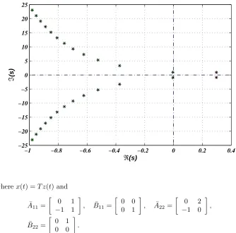
Figure 1. The roots of the characteristic equation of the subsys-tem (3.2) forτ= 3.2.
−1 −0.8 −0.6 −0.4 −0.2 0 0.2 0.4
−25 −20 −15 −10 −5 0 5 10 15 20 25
ℜ(s)
ℑ
(s)
wherex(t) =T z(t) and
¯ A11=
[ 0 1 −1 1
]
, B¯11=
[ 0 0 0 1
]
, A¯22=
[ 0 2 −1 0
] ,
¯ B22=
[ 0 1 0 0
] .
Now, we employ the direct method to each of the subsystems (3.2) and (3.3) sepa-rately. Subsystem (3.2) has a crossing frequency at s =±j and sgnW′(ω2) is zero
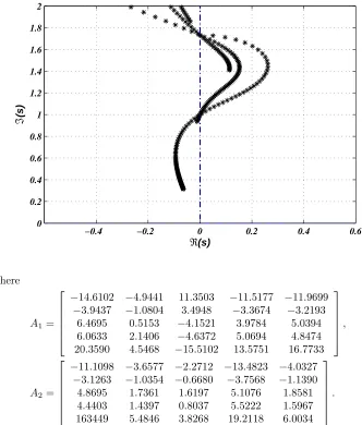
at this frequency. Therefore, the subsystem is unstable for allτ. The characteristic equation of subsystem (3.3) crosses the imaginary axis at s = ±√3j and s = ±j. The quantity sgnW′(ω2) is positive and negative at these frequencies, respectively.
Therefore, this subsystem is stable forπ < τ < √2π
3. Thus, the system (3.1) has two
stable poles for π < τ < √2π
3. The roots of the characteristic equation of the
sub-system (3.2) and the root locus of the subsystem (3.3) near the imaginary axis are plotted in Figure1and Figure2, respectively.
Example 3.2. Let us analyze the stability of the following LSDDE
˙
Figure 2. The root locus of the subsystem (3.3) near the imaginary axis for 0< τ <4.
−0.4 −0.2 0 0.2 0.4 0.6
0 0.2 0.4 0.6 0.8 1 1.2 1.4 1.6 1.8 2 ℜ(s) ℑ (s) where
A1=
−14.6102 −4.9441 11.3503 −11.5177 −11.9699 −3.9437 −1.0804 3.4948 −3.3674 −3.2193
6.4695 0.5153 −4.1521 3.9784 5.0394 6.0633 2.1406 −4.6372 5.0694 4.8474 20.3590 4.5468 −15.5102 13.5751 16.7733
,
A2=
−11.1098 −3.6577 −2.2712 −13.4823 −4.0327 −3.1263 −1.0354 −0.6680 −3.7568 −1.1390 4.8695 1.7361 1.6197 5.1076 1.8581 4.4403 1.4397 0.8037 5.5222 1.5967 163449 5.4846 3.8268 19.2118 6.0034
.
First, we decompose the system (3.4) into subsystems and then we apply the direct method to each of the subsystems to explore the stability analysis of the whole system. The columns of the full column rank matrix
E=
1.2775 −1.3977 0.6036 −0.4111 −0.5536 0.9967 −0.5480 0.4946 −1.9230 2.3550
constitute a two-dimensional (A1, A2)-invariant subspace. We may choose the
trans-formationT in (2.1) as
T =
0.1250 4.5000 0.6667 2.7500 0 1.4142 0.7500 1.6250 0 0.7071 3.0000 0.8571 0 4.4286 1.0000 −1.0000 0 2.0000 2.6667 −2.0000
0 1.7321 −1.0000 1.4142 0.4286 .
After applying this transformation to the system (3.4), we derive two subsystems as follows
˙
z1(t) = ¯A11z1(t) + ¯B11z1(t−τ), (3.5)
˙
z2(t) = ¯A22z2(t) + ¯B22z2(t−τ), (3.6)
wherex(t) =T z(t) and
¯ A11=
[ 0 1 −1 1
]
, B¯11=
[ 0 0 0 1
]
, A¯22=
01 00 −11
1 −1 1
,
¯ B22=
00 00 00
1 0 0
.
By applying the direct method, the subsystem (3.5) is always unstable while the subsystem (3.6) has two stable poles for 3.1416< τ <3.3077. For this subsystem the
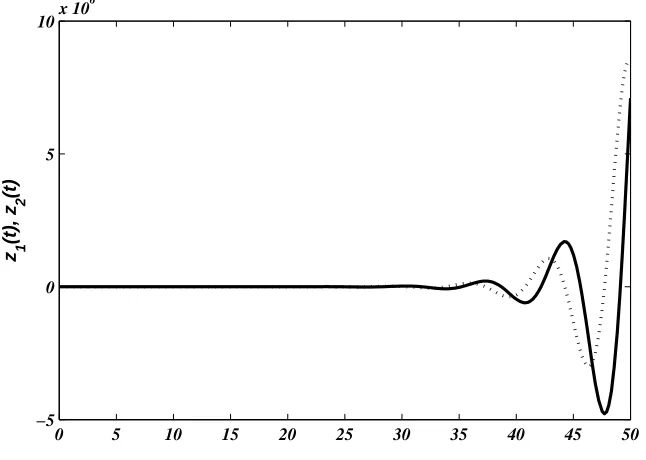
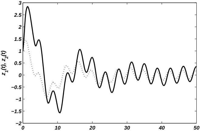
crossing frequencies ares =±j and s =±√1 +√2j. However, the direct method confirms that all characteristic roots of the system (3.4) are in the right half-plane, but by decomposing the system, we find out that the system has two stable poles 3.1416 < τ < 3.3077. The time domain response of the subsystem (3.5) for the constant initial condition z1(t) = 1,−τ ≤ t ≤ 0, is sketched in Figure 3. Also,
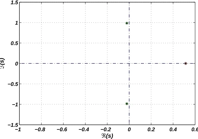
Figure4confirms that the subsystem (3.6) has two stable poles forτ= 3.2.
4. Stabilization of unstable time delay systems by the delayed feedback method
Figure 3. Time domain response of the subsystem (3.5). The solid line depictsz1(t) and dots displayz2(t).
0 5 10 15 20 25 30 35 40 45 50
−5 0 5
10x 10
6
z 1
(t), z
2
(t)
frequencies. Finally, the interval of time delay which the closed-loop system is stable can be obtained by the cluster treatment or direct methods.
As a concrete example, we consider the subsystem (3.2) that its stability analysis is done in the previous section. Let us consider the open-loop time delay system as
˙
z(t) =A1z(t) +A2z(t−3.2), (4.1)
where A1 and A2 are the same as ˜A11 and ˜B11, respectively. As we see earlier, the
system (4.1) had two unstable poles.
Now, our goal is the stabilization of the following closed-loop system by the delayed feedback method
˙
z(t) =A1z(t) +A2z(t−3.2)−BK(z(t)−z(t−τ)), (4.2)
where B = [1 0]T and K = [k1 k2]. As we said before, the stabilization of the
system (4.2) requires that the characteristic equation of the system (4.2) crosses the imaginary axis. Before going further, we propose the following lemma which gives us a necessary condition such thats=ωcj to be a root of the characteristic equation of the system (4.2).
Lemma 4.1. If s=ωcβ is a root of the characteristic equation of the system (4.2), where
Figure 4. The roots of the characteristic equation of the subsys-tem (3.6) forτ= 3.2.
−1 −0.8 −0.6 −0.4 −0.2 0 0.2 0.4 0.6
−1.5 −1 −0.5 0 0.5 1 1.5
ℜ(s)
ℑ
(s)
then the following relation holds
k2− |k2| −β(1−β)≤1−k1+|k1|(3 +β).
Proof. The proof is straightforward. By separating the real and imaginary parts of the characteristic equation of the system (4.2), we get the following relations fors=jω
1 + cos(ω(τ+ 3.2))k1−k1ωsin(ωτ)+(k1+k2) cos(ωτ)−k1cos(3.2ω)
−ωsin(3.2ω)−ω2−k1−k2= 0,
−sin(ω(τ+ 3.2))k1−k1ωcos(ωτ)−(k1+k2) sin(ωτ) +k1sin(3.2ω)
−ωcos(3.2ω) +k1(ω−1) = 0.
After applying the triangle inequality and using the famous inequalities |sin(x)|, |cos(x)| ≤1, the result follows immediately.
Now, we return to the stabilization process. According to Lemma4.1, if we choose k1 = 1 andk2=−5, then there are two crossing frequencies. These frequencies and
corresponding delays are
ωc1=±1.6564, τ11= 0.4540, τ12= 4.2473, . . . ,
Figure 5. Time domain response of the system (4.2) for τ = 0.5, k1= 1,k2=−5. The solid line depictsz1(t) and dots displayz2(t).
0 10 20 30 40 50
−2 −1.5 −1 −0.5 0 0.5 1 1.5 2 2.5 3
z 1
(t), z
2
(t)
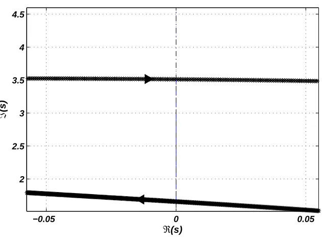
After obtaining the crossing frequencies, there are two scenarios which can be used to find the stability interval. The first one is the direct method. Using this method yields that the roots of the characteristic equation of the system move to the right half-plane at the larger crossing frequency and the next larger corresponds to stabilizing one. Therefore, the system (4.2) is stable for 0.4540< τ <0.9469. In the second scenario, we apply the cluster treatment method. The root tendency at the larger crossing frequency is 1 and it is−1 at the next one. Hence, the time delay system (4.2) is stable for 0.4540< τ <0.9469. In fact, these two approaches yield the same result. The time domain response and the root locus of the system (4.2) near the imaginary axis for τ = 0.5, k1 = 1 and k2 = −5 are illustrated in Figure 5 and Figure 6,
respectively.
5. Design controller via the delayed feedback method
Figure 6. The root locus of the system (4.2) near the imaginary axis for 0< τ <2.
−0.05 0 0.05
2 2.5 3 3.5 4 4.5
ℜ(s)
ℑ
(s)
the response. Here, we consider the subsystem (3.3) and we change the location of its dominant poles by the delayed feedback method.
Let
˙
z(t) =A1z(t) +A2z(t−3.2), (5.1)
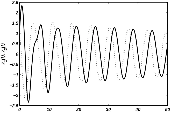
whereA1 andA2 are the same as ˜A11 and ˜B11, respectively. As we see in Figure7,
the settling time for this system is very high. To reduce the settling time of the system (5.1), we consider the following closed-loop system
˙
z(t) =A1z(t) +A2z(t−3.2)−BK(z(t)−z(t−τ)), (5.2)
whereB= [1 0]T andK= [k
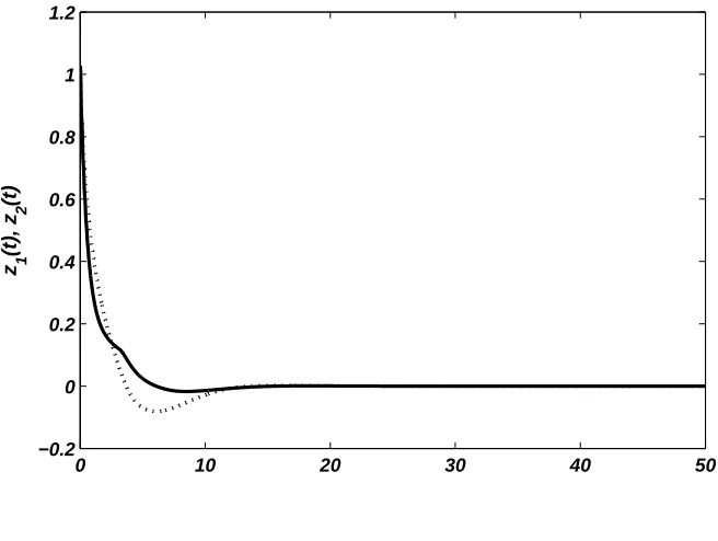
1 k2]. If we forces=−0.3254±0.3254jto be poles of
the system (5.2), the settling time is highly reduced. After doing this, we obtain two equations. Here, we have three parameters. We chooseτ freely. If we put τ = 0.1, then we havek1= 40.5925 and k2=−105.0352. The response of the system (5.2) is
plotted in Figure8.
6. Conclusion
Figure 7. Time domain response of the system (5.1). The solid line depictsz1(t) and dots displayz2(t).
0 10 20 30 40 50
−2.5 −2 −1.5 −1 −0.5 0 0.5 1 1.5 2 2.5
z 1
(t), z
2
(t)
of such systems, we decomposed them into several subsystems by an invertible trans-formation. Furthermore, we discussed the problem of stabilization of an LSDDE by the delayed feedback method. Also, we improved the performance of an LSDDE by this type of feedback. Further studies may be considered to evaluate the stability and stabilization of neutral type systems.
Acknowledgment
Figure 8. Time domain response of the system (5.2) for τ = 0.1, k1 = 40.5925 andk2 =−105.0352. The solid line depictsz1(t) and
dots display z2(t).
0 10 20 30 40 50
−0.2 0 0.2 0.4 0.6 0.8 1 1.2
z 1
(t), z
2
(t)
References
[1] C. Abdallah, P. Dorato, J. Benites-Read, and R. Byrne,Delayed positive feedback can stabilize oscillatory systems, In: Proceedings of American control conference, San Francisco, 1993, 3106– 3107.
[2] T. Dahms, P. H¨ovel, and E. Sch¨oll,Control of unstable steady states by extended time-delayed feedback, Phys. Rev. E,76(5) (2007), 056201.
[3] C. Dubi,Triangular realization of rational functions of N complex variables, Multidimens. Syst. Signal Process.,19(2008), 123–129.
[4] C. Dubi, An algorithmic approach to simultaneous triangularization, Linear Algebra Appl., 430(11) (2009), 2975–2981.
[5] E. Fridman,Introduction to time-delay systems: analysis and control, Birkhuser Basel, Springer Cham Heidelberg, 2014.
[6] I. Gohberg, P. Lancaster, and L. Rodman,Invariant subspaces of matrices with applications, SIAM, 1986.
[7] V. V. Gorbatsevich, A. L. Onishichik, and E. B. Vinberg, Structure of Lie groups and Lie Algebras, Springer-Verlag, Berlin, 1994.
[8] T. Kaczorek, Similarity transformation of matrices to one common canonical form and its applications to 2D linear systems, Int. J. Appl. Math. Comput. Sci.,20(3) (2010), 507–512. [9] W. H. Kown, G. W. Lee, and S. W. Kim, Performance improvement using time delays in
multivariable controller design, Int. J. Control,52(6) (1990), 1455–1473.
[11] P. Lancaster and M. Tismenetsky,The theory of matrices: second edition with applications, Elsevier, New York, 1985.
[12] L. Levsen and G. Nazaroff,A note on the controllability of linear time-variable delay systems, IEEE Trans. Automat. Contr.,18(2) (1973), 188–189.
[13] N. H. McCoy,On the characteristic roots of matric polynomials, Bull. Amer. Math. Soc.,42(8) (1936), 592–600.
[14] A. Mesbahi and M. Haeri,Decomposition of the time delay systems with one delay: The simul-taneous similarity of two matrices, Electrical and Electronics Engineering, 8th international conference on, (2013), 487–491.
[15] W. Michiels and S. I. Niculescu, Stability and Stabilization of Time-Delay Systems, SIAM, Philadelphia, 2007.
[16] Y. Mori, T. Mori, and Y. Kuroe,A solution to the common Lyapunov function problem for continuous-time systems, In: Proceedings of the 36th IEEE Conference on Decision and Control, 4(1997), 3530–3531.
[17] N. Olgac and R. Sipahi,An exact method for the stability analysis of delayed linear time-invariant (LTI) systems, IEEE Trans. Automat. Contr.,47(2002), 793–797.
[18] K. Pyragas,Delayed feedback control of chaos, Phil. Trans. R. Soc. A,365(2006), 2309–2334. [19] H. Radjavi,A trace condition equivalent to simultaneous triangularizability, Can. J. Math.,38
(1986), 376–386.
[20] H. Radjavi and P. Rosenthal,Simultaneous Triangularization, Springer-Verlag, New York, 2000. [21] Z. V. Rekasius, A stability test for systems with delays, In Join. Automat. Control Conf.,
(1980), 39–44.
[22] D. Shemesh,Common eigenvectors of two matrices, Linear Algebra Appl.,62(2009), 11–18. [23] R. N. Shorten and K. S. Narenda,On the stability and existence of common Lyapunov function
for stable linear switching systems, In: Proceedings of the 37th IEEE Conference on Decision and Control, (1998), 3723–3724.
[24] R. Sipahi, T. Vyhlidal, S. I. Niculescu, and P. Pepe,Time Delay Systems: Methods, Applications and New Trends, Springer-Verlag, 2012.
[25] F. Uhlig,Simultaneous block diagonalization of two real symmetric matrices, Linear Algebra Appl.,7(4) (1973), 281–289.