Vol 5, No. 1, (2015), pp 13-36
A two-phase variable neighborhood
search for solving nonlinear optimal
control problems
R. Ghanbari∗,A. Heydari and S. Nezhadhosein
Abstract
In this paper, a two-phase algorithm, namely IVNS, is proposed for solving nonlinear optimal control problems. In each phase of the algorithm, we use a variable neighborhood search (VNS), which performs a uniform distribution in the shaking step and the successive quadratic programming, as the local search step. In the first phase, VNS starts with a completely random initial solution of control input values. To increase the accuracy of the solution obtained from the phase 1, some new time nodes are added and the values of the new control inputs are estimated by spline interpolation. Next, in the second phase, VNS restarts by the solution constructed by the phase 1. The proposed algorithm is implemented on more than 20 well-known benchmarks and real world problems, then the results are compared with some recently proposed algorithms. The numerical results show that IVNS can find the best solution on 84% of test problems. Also, to compare the IVNS with a common VNS (when the number of time nodes is same in both phases), a computational study is done. This study shows that IVNS needs less computational time with respect to common VNS, when the quality of solutions are not different significantly.
Keywords: Nonlinear optimal control problem; Variable neighborhood search; Successive quadratic programming.
∗Corresponding author
Received 19 April 2014; revised 29 December 2014; accepted 6 January 2014 R. Ghanbari
Department of Applied Mathematics, Faculty of Mathematical Science, Ferdowsi Univer-sity of Mashhad, Mashhad, Iran. e-mail: [email protected]
A. Heydari
Department of Applied Mathematics, Payame Noor University, Mashhad, Iran. email: a [email protected]
S. Nezhadhosein
Department of Applied Mathematics, Payame Noor University, Tehran, Iran. email: s [email protected]
1 Introduction
Nonlinear optimal control problems (NOCP) are dynamic optimization prob-lems with many applications in process systems engineering, including the design of trajectories for the optimal operation of batch and semi-batch re-actors, economic systems, plasma physics, etc. [7].
Providing high-quality solutions with minimum computational time is the main issue for solving NOCPs. The numerical methods, direct [29] or indirect [46], usually have two main deficiencies, including low accuracy and conver-gence to a poor local solution. In direct methods, the quality of solutions depend on discretization resolution. These methods use control parametriza-tion to convert continuous problems to discrete problems, so they may have less accuracy. However, the adaptive strategies [8, 43] can overcome these defects, but they may be trapped by a local optimal, yet. In the indirect approach, the problem using Pontryagins minimum principle (PMP) is con-verted to two boundary value problems (TBVP) and then it can be solved by numerical methods such as shooting method [29]. These methods need the good initial guesses that lie within the domain of convergence. Therefore, numerical methods are not usually suitable for solving NOCPs, especially for large-scale and multimodal models.
Metaheuristics as the global optimization methods can overcome these problems, but they usually need more computational time, though they don’t really need good initial guesses and deterministic rules. Several researchers have used metaheuristics to solve optimal control problems. For instance, Michalewicz et al. [34] applied floating-point Genetic algorithms (GA) to solve discrete time optimal control problems, Yamashita and Shima [52] used the classical GAs to solve the free final time optimal control problems with terminal constraints. Abo-Hammour et al. [1] used continuous GA for solv-ing NOCPs. Recently, Sun et al. [47] proposed a hybrid improved GA, for solving NOCPs and applied it for chemical processes. Moreover, the other usages of GA for optimal control problems can be found in [44,45]. Modares and Naghibi-Sistani [37], proposed a hybrid algorithm by integrating an im-proved Particle Swarm Optimization (PSO) with a successive quadratic pro-gramming (SQP), for solving NOCPs. Lopez-Cruz et al. [14], applied Differ-ential Evolution (DE) algorithms for solving the multimodal optimal control problems. Recently, Ghosh et al. [22] developed an ecologically inspired op-timization technique, called Invasive Weed Opop-timization (IWO), for solving optimal control problems. The other well-known metaheuristic algorithms which are used for solving NOCPs are Genetic Programming (GP) [30], PSO [3,4], Ant Colony Optimization (ACO) [48] and DE [31,50].
of combinatorial optimization and global optimization problems which uses neighborhood changes and uniform distributions in search procedure. Un-like many other metaheuristics, it is simple and requires few parameters [32]. Mladenovi´c et al. [36] proposed a general VNS for solving continuous opti-mization. Moreover, VNS was used for solving several optimization problem [25] such as mixed integer programming [26], vertex weightedk−cardinality tree problem [10], and scheduling problem [13].
In this paper, VNS uses a uniform distribution in the shaking step and the SQP [39], as the local search step (similar to [37]). SQP is an iterative algorithm for solving NLP, which uses gradient information. Furthermore, SQP is used for solving NOCPs alone [6,18].
For performing VNS to solve an NOCP, the time interval is uniformly divided by using a constant number of time nodes. Next, in each of these time nodes, the control variable is approximated by a scalar matrix of control input values. Thus, an infinite dimensional NOCP is changed to a finite dimensional nonlinear programming (NLP). Now, we encounter two conflict situations: the quality of the global solution and the needed computational time. In other words, when the number of time nodes is increased then we expect the quality of the global solution to increase but we know that in this situation the computational time is increased dramatically. In other situation, we consider less number of time nodes to reduce the computational but we may find a poor local solution. To conquer these problems, IVNS, performs VNS in two phases. In the first phase of IVNS (exploration phase), to decrease the computational time and to find a promising solution in the search space, VNS uses a less number of time nodes. Next to increase the quality of the solution obtained from Phase 1, the number of time nodes is increased. Using the obtained solution in Phase 1, the values of the new control inputs are estimated by spline interpolation. Next, in the second phase of IVNS (exploitation phase), VNS uses the solution constructed by the above procedure, as an initial solution. A computational study in our numerical experiments shows that there is a significant difference between the computational time of IVNS and a common VNS, that uses all time nodes from the beginning.
2 Problem formulation
NOCPs are formulated as optimization problems by the performance index as the objective function and differentiate equations as constraints that called dynamic optimizations. There are several types of these problems e.g. track-ing problem, terminal control problem and time minimization problem [29]. We consider nonlinear bounded continuous-time control problems in which a vector of control functions,u, is exerted over the planning horizon [t0, tf].
The particular problem considered is that of finding the control input vector
u(t)∈Rmthat minimizes the performance index:
min J =ϕ(x(tf), tf) + ∫ tf
t0
g(x(t), u(t), t)dt (1)
subject to:
˙
x(t) =f(x(t), u(t), t), (2)
c(x(t), u(t), t) = 0, (3)
d(x(t), u(t), t)≤0, (4)
ψ(x(tf), tf) = 0, (5)
x(t0) =x0, t∈[t0, tf]. (6)
where x(t) ∈ Rn denotes the state vector for the system and x
0 ∈ Rn is
the initial state. The functions f : Rn+m×R → Rn, g : Rn+m×R →
R, c : Rn+m×R →Rnc, d: Rn+m×R → Rnd, ψ : Rn×R → Rnψ and
ϕ:Rn×R→Rare assumed to be sufficiently smooth on appropriate open sets. The cost function (1) must be minimized subject to dynamic (2), control and state equality constraints (3), control and state inequality constraints (4), the initial condition (6) and the final state constraints (5).
3 Proposed algorithm
Here, we propose IVNS for solving NOCPs. Before providing a description of IVNS, we introduce VNS.
3.1 VNS algorithm
local minima. It explores distant neighborhoods of the current incumbent solution, and moves from there to a new one if and only if an improvement is necessary. Local search method is applied repeatedly to get in the neigh-borhood to local optima [36]. Here, the implemented VNS in each phase has the following steps:
Initialization: The time interval is divided intoNt−1 subintervals using time
nodest0, . . . , tNt−1 and then control input values are computed (or selected
randomly) as control points. This can be done by the following stages:
1. Lettk=t0+kh,whereh= tf−t0
Nt−1, k= 0,1, . . . , Nt−1, be time nodes,
wheret0 andtf are the initial and final times, respectively.
2. The corresponding control input value at each time node, tk, k =
0, . . . , Nt−1 is an m×1 vector, uk = [u (k) 1 , . . . , u
(k)
m]T, having the
following components:
u(k)i =ulef t,i+ (uright,i−ulef t,i).ri, i= 1,2, . . . , m (7)
where ri is a random number in [0,1] with uniform distribution and
ulef t, uright∈Rmare the lower and the upper bound vectors of control
input values, which can be given by the problem’s definition or the user (e.g. see the NOCPs No. 7 and 8 in Appendix, respectively).
u= [uk]Nk=0t−1 is called control input matrix.
Evaluation: The corresponding state matrix with the control input matrix,
u, is ann×Ntmatrix,x= [xk]k=0Nt−1, wherexk,k= 0,1, . . . , Nt−1, is ann×1
vector as the (k+ 1)-th column of state matrix, and can approximately be computed by the forth Runge-Kutta method on dynamic system (2) with the initial condition (6). Without loss of generality, assume m= 1 (for general case it can be extended easily). So, the evaluation procedure is as follows:
xk=xk−1+
1
6(l1+ 2l2+ 2l3+l4), k= 1,2, . . . , Nt−1 (8)
where
l1=hf(xk, uk, tk), l2=hf(xk+
l1
2, uk+
h
2, tk)
l3=hf(xk+
l2
2, uk+
h
2, tk), l4=hf(xk+l3, uk+h, tk)
where uk = u(tk) and xk = x(tk), with initial condition x(t0) = x0. To
approximate the performance index, the composite Simpson’s method [5], is used. Then, the performance index in (1),J, is approximated by ˜Jas follows:
J ≃J˜=ϕ(xNt−1, tNt−1) + h
3(f0+ 4
[Nt2∑]−1
i=1
f2i+1+ 2 [Nt2∑]−1
i=0
where fk = f(xk, uk, tk), k = 0,1, . . . Nt−1. If NOCP includes equality
or inequality constraints e.g. (3) or (4), or has final state constraints, given by (5), then we add some penalties to the corresponding fitness value of the solution. Finally, we assignI(u) touas the fitness value as follows:
I(u) = ˜J+
nd
∑
l=1 N∑t−1
j=0
M1lmax{0, dl(xj, uj, tj)}+ nc
∑
h=1 N∑t−1
j=0
M2hc2h(xj, uj, tj)
+
nψ
∑
p=1
M3pψp2(xNt−1, tNt−1) (10)
where M1 = [M11, . . . , M1nd]
T, M
2 = [M21, . . . , M2nc]
T and M 3 =
[M31, . . . , M3nψ]
T are big numbers, as the penalty coefficients, forc
h(., ., .), h=
1,2, . . . , nc,dl(., ., .), l= 1,2, . . . , nd, andψp(., .), p= 1,2, . . . , nψ defined in
(3), (4) and (5), respectively.
The fitness value in (10), can be viewed as a nonlinear objective function with the decision variable asu= [u0, u1, . . . , uNt−1]. This cost function with
upper and lower bounds of input signals construct a finite dimensional NLP problem as follows:
min I(u) =I(u0, u1, . . . , uNt−1) s.t
ulef t≤uj≤uright, j= 0,1, . . . , Nt−1 (11)
Neighborhood: VNS uses at most kmax neighborhoods, Vr1, . . . , Vrkmax, in
whichri, i= 1, . . . , kmaxis the radii of i-th neighborhood,Vi, of the control
input matrix u.
Shaking: In this stage, using a uniform distribution, a random direction matrixd∈[−1,1]m×Nt is firstly generated and then a random solution, ¯u, is
selected in thek-th neighborhood,Vk, by the following equation:
¯
u=u+d.α.(r+k−1) (12)
where r∈[0,1] is a random number, k is the index of neighborhood andα
is the parameter of radii.
Local search: In this stage, SQP algorithm [9,39] is performed on the NLP (11), using ¯u0 = ¯u, constructed in (12), as the initial solution when the maximum number of iteration issqpmaxiter.
as the search direction in the line search procedure. For the NLP (11), the principal idea is the formulation of a QP subproblem based on a quadratic approximation of the Lagrangian function asL(u, λ) =I(u) +λTh(u), where
the vectorλis Lagrangian multiplier andh(u) return the vector of, inequality constraints evaluated at u. The QP is obtained by linearizing the nonlinear functions as follows:
min1 2d
TH(¯uk)d+∇I(¯uk)Td
∇h(¯uk)Td+h(¯uk)≤0
Similar to [18], here a finite difference approximation is applied to compute the gradient of the cost function and the constraints, with the following components
∂I ∂uj
=I(...uj+δ...)−I(uj)
δ , j= 0,1, . . . , Nt−1 (13)
where δ is the double precision of machine. So, the gradient vector is
∇I = [∂u0∂I , . . . ,∂u∂I Nt−1]
T. Also, at each major iteration a positive definite
quasi-Newton approximation of the Hessian of the Lagrangian function, H, is calculated using the BFGS method [39], whereλi, i= 1, ..., m, is an
esti-mated of the Lagrange multipliers. The general procedure of SQP, for NLP (11), is as follows:
1. Given an initial solution ¯u0. Letk= 0.
2. Construct the QP subproblem (13), based on ¯u0, using the
approxima-tions of the gradient and the Hessian of the the Lagrangian function.
3. Compute the new point as ¯uk+1 = ¯uk+dk, where dk is the optimal
solution of the current QP.
4. Let k=k+1 and go to step 2.
Here, in IVNS, SQP is used as the local search step, and we use the maximum number of iterations as the main criterion for stopping SQP. In other words, we terminate SQP when it converges either to local solution or the maximum number of SQP’s iterations is reached.
Terminal conditions: The algorithm is terminated when the number of neigh-borhoods reached to kmax or the difference between cost functions in two
Algorithm 1 VNS algorithm
{Initialization}Input the number of time nodesNt, the maximum
num-ber of iteration for SQP,sqpmaxiter, a maximum number of neighborhood,
kmax, the parameter of radii, α defined in (12), the lower and the upper
bound vectors of control input valuesulef t, uright, an initial solution,u∗,
andε. Letk= 1.
{Evaluation}Evaluate the fitness of the initial solution,u∗ and letI∗=
I(u∗), whereI(.) is defined in (10). repeat
{Shaking}Using (12), selectuin k-th neighborhood ofu∗.
{Local search}Perform SQP algorithm on the NLP (11), usinguas the initial solution when the maximum number of iteration issqpmaxiter. Let ¯ube the obtained solution, ¯I=I(¯u) ande=|I¯−I∗|.
if I < I¯ ∗then
Letu∗= ¯u,I∗= ¯I andk= 1. else
Letk=k+ 1 end if
untilk > kmaxor e < ε
Returnu∗as the approximate solution,x∗as the corresponding state and the corresponding fitnessI∗.
3.2 IVNS
We now give a new algorithm, IVNS, which is a two-phase direct metaheuris-tic approach. The main idea of IVNS is to find promising solution of the search space using the computational time as few as possible.
IVNS has two main phases (as discussed in Section1). In the first phase, we perform VNS (Algorithm 1) with a completely random initial solution constructed by (7). Since the main goal in this phase is to find the promising solution in the search space, we use a few number of time nodes.
Next, to maintain the property of the solution given in Phase 1 and to increase the accurately of this solution, we add some additional time nodes. Thus, we increase time nodes fromNt1 in the Phase 1 to Nt2 in the Phase
2. To use the information of the obtained solution from Phase 1 in the construction of the initial solution for Phase 2, we use Spline interpolation to estimate the values of the control inputs based on the curve obtained from the Phase 1. In the second phase, VNS restarts with this solution. Finally, IVNS is given in Algorithm 2.
Algorithm 2 IVNS
InitializationInputulef tanduright.
{Phase 1}Perform VNS (Algorithm1) with a random initial solution and using the parametersNt1, sqpmaxiter, kmax, αandε. (see Algorithm1)
{Constructing an initial solution for Phase 2} Increase time nodes uniformly to Nt2 and estimate the corresponding control input values by
using Spline interpolation on the obtained solution from Phase 1.
{Phase 2}Restart VNS (Algorithm1) with the constructed initial solution and usingNt2, sqpmaxiter, kmax, αandε. (see Algorithm1)
mentioned that all metaheuristics are practical algorithms that are interesting for their numerical behaviour, [16].
4 Numerical experiments
In this Section, to investigate the efficiency of IVNS, more than 20 well-known and real world NOCPs, as benchmark problems, are considered. These problems are selected with single control signal and multi control signals.
The numerical behaviour of the algorithms can be studied from two points of view: the performance index and the final state constraints. Let J be the value of the performance index and ψ= [ψ1, . . . , ψnψ]
T, defined in (5),
and ϕf = ∥ψ∥2 be the vector of final state constraints and the error ofψ,
respectively. Now, the absolute errors for J andϕf, are defined as follows:
EJ =|J−J∗|, Eψ=|ϕf−ϕ∗f| (14)
whereJ∗andϕ∗f =∥ψ∗∥2are the best obtained solutions among the methods,
or the exact solutions (when exist). To control the accuracy study, we now define a new criterion, called factor, to compare the numerical behaviour of the algorithms as follows:
Kψ=EJ+Eψ (15)
where EJ andEψ are defined in (14). Note that Kψ shows the summation
of two important errors. Thus, based onKψ we can study the behaviour of
algorithms on the quality and feasibility of given solutions, simultaneously. To solve any NOCP described in the Appendix, we must know IVNS’s parameters including Nt1, Nt2, kmax, α, εandsqpmaxiter (see Algorithm
1), and the problem’s parameters includingulef t, urightandMi, i= 1,2,3, in
subsection or in Table 2. Because of the stochastic nature of the proposed algorithm, 12 different runs were done, for each NOCP, and the best result are reported in Table1. The best value of each column is highlighted in the bold. The reported numerical results for each algorithm included the value of performance index,J, the absolute error ofJ andEJ, are defined in (14).
The final state constraints,ψ= [ψ1, . . . , ψnψ]
T, the two-norm or error of the
final state constraints, ϕf, the absolute error of ϕf and Eψ, are defined in
(14), and the factorKψ is defined in (15).
The algorithm was implemented in Matlab R2011a environment on a Notebook with Windows 7 Ultimate, CPU 2.53 GHz and 4.00 GB RAM. Also, to implement SQP in the proposed algorithm, as the local search, we used ‘fmincon’ in Matlab when the ‘Algorithm’ was set to ‘SQP’.
In Subsection4.1, the numerical results of IVNS are compared with exact solutions. Also, for comparing IVNS with metaheuristics and numerical algo-rithms in two Subsections4.2and4.3, we consider 22 NOCPs. Their models are described in the Appendix, which are presented in terms of equations (1)-(6). The numerical results are summarized in Table1. Details of these comparisons are given in the following subsection.
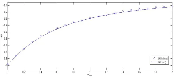
4.1 Comparison with the exact solution
Consider the nonlinear system state equations [24]
˙
x1=x32,
˙
x2=u
The cost functional to be minimized, starting from the initial statesx1(0) = 0
andx2(0) = 1, is
J = 4x1(2) +x2(2) + 4 ∫ 2
0
u2(t)dt
The exact trajectories of the problem, from PMP, are x∗1(t) = 25 −5(t+2)64 5
and x∗2(t) = (t+2)4 2, with the exact control signal u∗(t) = − 8
(t+2)3. Also the
exact value of the performance index is J∗ = 3.35. For the proposed algo-rithm, IVNS’s parameters are set asNt1 = 15, Nt2 = 21, ε= 10−6 and the
problem’s parameters are set as ulef t =−1 and uright =−14. The IVNS’s
solution for the problem isJ = 3.3418, thus,EJ=Kψ= 0.0082.
Figure1shows the graphs of the exact and the obtained trajectories, for
x1 and x2, and Figure 2 shows the graphs of the exact and the obtained
Figure 1: The exact and the obtained trajectories of (a)x1and (b)x2, for the NOCP in subsection4.1
Figure 2: The exact and the obtained control signals for the NOCP in subsection4.1
4.2 Comparison with metaheuristic algorithms
TCCR problem [47]
The first NOCP in the Appendix is a chemical process of Temperature Con-trol for Consecutive Reaction, TCCR, which is an unconstrained two-state variable mathematical system. The objective is to obtain the optimal tem-perature profile that maximizes the yield of the temtem-perature product B at the end of operation in a batch reactor, where the reaction A → B → C
is occurred. The state variables, x1 and x2 are the concentration of A and
B, respectively, and the control variable uis the temperature. The problem solved by HIGA [47], which was more accurate than ACO [40] and iterative ACO [53]. From Table1, we can see that the numerical behaviour of IVNS is better than HIGA.
VDP problem [1,17]
The second NOCP in the Appendix is Van Der Pol, VDP, problem which has two state variables and one control variable. VDP problem has a final state constraint, which isψ=x1(tf)−x2(tf)+1 = 0. The problem solved by CGA
[1] and IVNS. From [1], the norm of final state constraint for the CGA equals
ϕ∗f = 2.67×10⁻¹¹, however, this value for IVNS equals ϕf = 3.04×10⁻⁹.
So, the factor Kψ for these methods can be seen in the sixth column of the
Table 1. Note that the Kψ of IVNS, 3.01×10⁻⁹, is less than CGA’s Kψ,
3.0×10⁻⁴. From Table1, it is seem that IVNS can achieved more suitable
solution than CGA.
CRP problem [1,29]
The third NOCP in the Appendix is a mathematical model of Chemical Re-actor Problem, CRP, which has two state variables and one control variable. The control variable is the flow of a coolant through a coil inserted in the reactor that controls the first-order irreversible exothermic reaction taking place in the reactor. The state variables,x1 andx2, are the deviations from
the steady-state temperature and concentration, respectively. The numerical results of IVNS and CGA are shown in the third row of Table1. CRP prob-lem has two final state constraints,ψ= [x1, x2]T. From [1], the norm of final
state constraints for CGA, equals ϕ∗f = 7.57×10⁻¹⁰, when IVNS’s norm of final state constraints isϕf = 2.50×10⁻⁸. But, the correspondingKψof two
FFRP problem [1,18]
The fourth NOCP in the Appendix is Free Floating Robot Problem, FFRP, which has six state variables and four control variables. It was solved by CGA [1]. FFRP problem has six final state constraints,ψ= [x1−4, x2, x3−
4, x4, x5, x6]T. The norm of final state constraints for IVNS isϕ∗f = 4.61×
10−4, however, this value, from [1], for CGA isϕ
f = 4.65×10⁻³. From Table
1, we can see the numerical behaviour of IVNS is better than CGA, also it is clear that the obtained values ofJ, EJ, ϕf, Eψ and Kψ from IVNS are
better than CGA.
CSTCR problem [37]
The fifth NOCP in the Appendix is a model of a nonlinear Continuous Stirred-tank Chemical Reactor, CSTCR. It has two state variablesx1(t) andx2(t), as
the deviation from the steady-state temperature and concentration, and one control variable u(t), which represents the effect of the flow rate of cooling fluid on chemical reactor. The objective is to maintain the temperature and concentration close to steady-state values without expending large amount of control effort. Also, this is a benchmark problem in the handbook of test problems in local and global optimization [20], which is a multimodal optimal control problem [2]. It involves two different local minima. The values of the performance indices, for these solutions, equal 0.244 and 0.133. The numerical results of IVNS, with the parameters in Table2, are compared with IPSO [37], and numerical methods in [2, 14]. From the results of the fifth row of Table1, we can see that IVNS is the best.
MSNIC problem [37]
In the sixth NOCP in the Appendix, a Mathematical System with Nonlinear Inequality Constraint, MSNIC, is considered. It includes an inequality con-straint, d(x, t) =x2(t) + 0.5−8(t−0.5)2≤0. From the sixth row of Table
1, we can see that the obtained value of the performance index, for IVNS is J∗ = 0.1720, which is better than IPSO’s, 0.1727, and other numerical methods given in [23,33].
4.3 Comparison with numerical algorithms
state constraints are not reported. But these values are reported for IVNS in Table1.
Comparison with B´ezier [21]
The NOCP No. 7, in the Appendix, has exact solution, i.e. the exact value of performance index equalsJ∗=−5.5285 [49]. This problem has an inequality constraint as d(x, t) = −6−x1(t) ≤0. It has been solved by a numerical
method, proposed in [21], called B´ezier, and the proposed algorithm, IVNS, with the parameters in Table2. From seventh row of Table1, the obtained value of the performance index from IVNS is better and more accurate than B´ezier method.
Comparison with HPM [15], DTM [41] and ADM [19]
In this subsection, the results of IVNS with the parameters given in Table2, are compared with HPM [15], DTM [41] and ADM [19]. For NOCP No. 8 in the Appendix, which is a constraint nonlinear model, the numerical results are compared with HPM. This NOCP has a final state constraint as
ψ=x−0.5 = 0.
From [15], the norm of final state constraint for HPM is ϕf = 4.2×10⁻⁶,
however, this value for IVNS equalsϕ∗f = 6.83×10⁻¹¹. From Table1, it is clear that the obtained values of the performance index, the norm of final state constraint andKψ from IVNS are better than HPM’s.
The problem No. 9 in the Appendix is a linear quadratic optimal control which has been solved by two numerical methods, DTM [41] and ADM [19]. Using the approximate values of k(t), which is used to achieve the optimal control signal by linear feedback control asu(t) =−k(t)x(t), the performance index could be calculated. The exact solution, from PMP, equalsJ∗= 0.1929. From Table1, the values ofEJ andKψ, for IVNS, with the same number of
points,Nt2 = 15, equals 0.0052, which is less than DTM and ADM methods,
(0.0087).
Comparison with SQP and SUMT
For NOCPs No. 10-22 in the Appendix, the numerical results of IVNS (the parameters are given in Table2) are compared with SQP and SUMT meth-ods. All these problems are described in [18]. For SQP and SUMT, the status of the final state constraints were not reported, so, we replaced the values of
ϕf instead ofEψ, in Table 1. Also, in computation of the factor, Kψ, the
results (given in Table 1) show that IVNS could find more accurate results for performance indexJ, and the factorKψ, perspective.
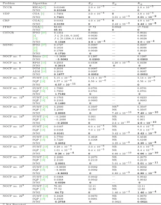
Table 1: The best of numerical results for 12 different runs of NOCPs described in Appendix
Problem Algorithm J EJ Eψ Kψ
TCCR HIGA[47] 0.61046 2.0×10⁻⁵ — 2.0×10⁻⁵
IVNS 0.61048 0 — 0
VDP CGA [1] 1.7404 3.0×10⁻⁴ 0 3.0×10⁻⁴ IVNS 1.7401 0 3.01×10⁻⁹ 3.01×10⁻⁹
CRP CGA[1] 0.0163 4.0×10⁻⁴ 0 4.0×10⁻⁴ IVNS 0.0159 0 2.42×10⁻⁸ 2.42×10⁻⁸
FFRP CGA[1] 83.63 17.72 0.0042 17.7242
IVNS 65.91 0 0 0
CSTCR IPSO [37] 0.1354 0.0024 — 0.0024 [2] J∈[0.135,0.245] 0.0020 — 0.0020 [14] J∈[0.1358,0.1449] 0.0028 — 0.0028 IVNS 0.1328 2.0×10⁻⁴ — 2.0×10⁻⁴
MSNIC IPSO [37] 0.1727 0.0007 — 0.0007
[23] 0.1816 0.0096 — 0.0096
[33] 0.1769 0.0049 — 0.0049
IVNS 0.1720 0 — 0
NOCP no. 7 B´ezier [21] −5.3898 0.1387 — 0.1387 IVNS −5.5082 0.0203 — 0.0203
NOCP no. 8 HPM [15] 0.2353 0.0338 4.20×10⁻⁶ 0.0338
IVNS 0.2015 0 0 0
NOCP no. 9 DTM [41] 0.2016 0.0087 — 0.0087 ADM [19] 0.2016 0.0087 — 0.0087 IVNS 0.1877 0.0052 — 0.0052
NOCP no. 10b SUMT [18] 5.15×10⁻⁶ 5.14×10⁻⁶ — 5.14×10⁻⁶ SQP [18] 6.57×10⁻⁶ 6.56×10⁻⁶ — 6.56×10⁻⁶
IVNS 6.57×10⁻¹¹ 0 — 0
NOCP no. 11b SUMT [18] 1.7980 0.0791 — 0.0791 SQP [18] 1.7950 0.0761 — 0.0761
IVNS 1.7189 0 — 0
NOCP no. 12b SUMT [18] 0.1703 0.0223 — 0.0223 SQP [18] 0.2163 0.0683 — 0.0683
IVNS 0.1480 0 — 0
NOCP no. 13b SUMT [18] 3.2500 0.3507 NRa 0.3507 SQP [18] 3.2500 0.3507 NR 0.3507 IVNS 2.8993 0 7.49×10⁻¹⁰ 7.49×10⁻¹⁰
NOCP no. 14b SUMT [18] −0.2490 0.001 NR 0.001 SQP [18] −0.2490 0.001 NR 0.001 IVNS −0.2500 0 2.6×10⁻¹⁰ 2.6×10⁻¹⁰
NOCP no. 15b SUMT [18] 0.0167 6.0×10⁻⁴ NR 6.0×10⁻⁴ SQP [18] 0.0168 7.0×10⁻⁴ NR 7.0×10⁻⁴ IVNS 0.0161 0 3.42×10⁻⁹ 3.42×10⁻⁹
NOCP no. 16b SUMT [18] 3.7700 0.4648 NR 0.4648 SQP [18] 3.7220 0.4168 NR 0.4168 IVNS 3.3052 0 3.35×10⁻⁸ 3.35×10⁻⁸
NOCP no. 17b SUMT [18] 9.29×10⁻⁴ 3.0×10⁻⁶ NR 3.0×10⁻⁶ SQP [18] 1.01×10⁻³ 8.4×10⁻⁵ NR 8.4×10⁻⁵ IVNS 9.26×10⁻⁴ 0 6.66×10⁻¹⁰ 6.66×10⁻¹⁰
NOCP no. 18b SUMT [18] 2.2080 0.2079 NR 0.2079 SQP [18] 2.2120 0.2119 NR 0.2119 IVNS 2.0001 0 5.01×10⁻¹¹ 5.01×10⁻¹¹
NOCP no. 19b SUMT [18] −8.8690 0.0002 NR 0.0002 SQP [18] −8.8690 0.0002 NR 0.0002 IVNS −8.8692 0 6.89×10⁻⁹ 6.89×10⁻⁹
NOCP no. 20b SUMT [18] 0.0368 0.0042 — 0.0042 SQP [18] 0.0368 0.0042 — 0.0042
IVNS 0.0326 0 — 0
NOCP no. 21b SUMT [18] 76.83 12.11 NR 12.11 SQP [18] 77.52 12.80 NR 12.80 IVNS 64.72 0 1.46×10⁻⁴ 1.46×10⁻⁴
NOCP no. 22b SUMT [18] 0.3428 0.0670 NR 0.0670 SQP [18] 0.3439 0.0681 NR 0.0681 IVNS 0.2758 0 0.0021 0.0021 aNot Reported.
bWe here consider,Eψ=ϕf for IVNS, and for SQP and SUMT methods,Eψ= 0
(since the values were not reported, we consider the best possible situation for SQP and SUMT).
zero for all test problems. It shows that IVNS provides robust results with respect to the other methods.
To have a more careful comparison, we computed the Gap between the performance index’s value of the algorithms and the best obtained perfor-mance index’s value. In other words, let J be the obtained value of the performance index of an algorithm. Now, similar to [51], we define the Gap as follows:
Gap(J) =|J−J
∗
J∗ | (16)
From Table1, the mean values of Gap for IVNS, SQP and SUMT, on NOCPs No. 10-22, are 0, 7.69e+ 3 and 6.02e+ 3, respectively. Thus it is obvious that, IVNS gave more better solution in comparison with SQP and SUMT. We believe that this is due to the fact that IVNS tries to find the global solution but SQP and SUMT didn’t escape from a local minimum.
To compare with the CGA (as a global search algorithm), from Table
1, we see that the mean values of the Gap for CGA is 0.0981. Thus, we can see IVNS is 100 percent better than CGA from Gap perspective. This result shows that IVNS’s estimations of global minimal is better than CGA’s estimation. Therefore, based on these numerical study, we can conclude that IVNS outperforms than CGA.
The mean values of violation of the norm of the final state constraints,ϕf,
for IVNS is 1.16×10⁻⁴. Therefore, it is evident that IVNS is more robust. Also, the mean value ofϕf for IVNS and CGA are 1.53×10⁻⁴and 1.55×10⁻³,
respectively, on NOCPs no. 2-4. Thus, we can say that the feasibility of the solutions given by IVNS and CGA are competitive. Therefore, it is seen that IVNS could provide very suitable solutions with respect to the optimality and feasibility criteria. Also, the mean of the factor, Kψ, for IVNS equals
1.28×10⁻³. For NOCPs No. 10-22 the mean of factor for IVNS, SQP
and SUMT equals 1.76×10⁻⁴, 1.0768 and 1.0272, respectively. Therefore,
we can say that IVNS outperform well-known numerical methods. Since, the computational times of the most algorithms were not reported thus we didn’t give the computational times of IVNS in Table 1. But, the details of the computational time of IVNS is given in Table3that will be discussed in Section5.
5 Comparison with a common VNS
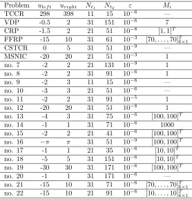
Table 2: The parameters of IVNS for NOCPs described in the Appendix
Problem ulef t uright Nt1 Nt2 ε Mi
TCCR 298 398 11 15 10−6 —
VDP -0.5 2 31 151 10−6 7
CRP -1.5 2 21 51 10−8 [1,1]T
FFRP -15 10 31 61 10−3 [70, . . . ,70]T6×1
CSTCR 0 5 31 51 10−9 —
MSNIC -20 20 21 51 10−3 1
no. 7 -2 2 21 131 10−9 1
no. 8 -2 2 31 91 10−6 1
no. 9 -2 3 11 15 10−6 —
no. 10 -3 3 21 51 10−6 —
no. 11 -2 2 31 91 10−5 1
no. 12 -20 20 31 51 10−8 1
no. 13 -4 3 31 75 10−6 [100,100]T
no. 14 -1 1 31 71 10−6 1000
no. 15 -2 2 21 41 10−6 [100,100]T
no. 16 −π π 31 51 10−9 [100,100]T
no. 17 -1 1 21 35 10−6 [10,10]T
no. 18 -5 5 31 151 10−6 [10,10]T
no. 19 -30 30 31 171 10−6 [100,100]T
no. 20 -1 1 31 171 10−6 —
no. 21 -15 10 31 71 10−6 [70, . . . ,70]T 6×1
no. 22 -15 10 21 91 10−6 [10, . . . ,10]T 6×1
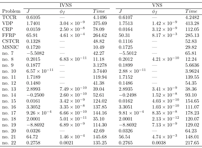
Nt2, is applied. For these methods, 35 different runs, for each NOCP in
the Appendix, were made with the same parameters. The influence of these methods investigated for these NOCPs on the dependent outputs consist of performance index,J, the factor,ϕfand required computational time,T ime.
The results are given in Table3.
From Table3, we observe that the two-phase method has no significant effect onJ, ϕf. But the two-phase method, IVNS, needs less computational
time than the common VNS, significantly (except NOCP No. 16). Therefore, based on this computational study, we can conclude that the usage of two-phase VNS can decrease the computational time, significantly, without loss of quality of solution.
6 Conclusion
Table 3: The best numerical results for NOCPs in Appendix, using IVNS and common VNS
IVNS VNS
Problem J ϕf T ime J ϕf T ime
TCCR 0.6105 — 4.1496 0.6107 — 4.2482 VDP 1.7401 3.04×10⁻⁹ 375.69 1.7513 1.42×10⁻⁹ 413.28
CRP 0.0159 2.50×10⁻⁸ 78.09 0.0164 3.12×10⁻⁹ 112.05
FFRP 65.91 4.61×10⁻⁴ 264.62 50.31 8.17×10⁻³ 285.13
CSTCR 0.1328 — 48.82 0.1116 — 52.83
MSNIC 0.1720 — 10.49 0.1725 — 29.82
no. 7 −5.5082 — 42.27 −5.5012 — 65.81 no. 8 0.2015 6.83×10⁻¹¹ 11.18 0.2012 4.21×10⁻¹⁰ 12.24
no. 9 0.1877 — 3.1278 0.1899 — 5.6636 no. 10 6.57×10⁻¹¹ — 3.7440 2.88×10⁻¹¹ — 3.9624
no. 11 1.7189 — 119.94 1.7152 — 139.55 no. 12 0.1480 — 41.38 0.1486 — 54.35 no. 13 2.8993 7.49×10⁻¹⁰ 39.04 2.8935 3.41×10⁻⁹ 38.36
no. 14 −0.2500 2.60×10⁻¹⁰ 52.61 −0.2498 1.52×10⁻⁸ 93.10
no. 15 0.0161 3.42×10⁻⁹ 124.02 0.0162 4.03×10⁻¹⁰ 154.65
no. 16 3.3052 3.35×10⁻⁸ 137.85 3.3051 1.03×10⁻¹⁰ 111.07
no. 17 9.26×10⁻⁴ 6.66×10⁻¹⁰ 144.16 9.81×10⁻⁴ 8.35×10⁻⁸ 178.23
no. 18 2.0001 5.01×10⁻¹¹ 35.10 2.0001 2.13×10⁻¹² 120.07
no. 19 −8.8692 6.89×10⁻⁹ 114.30 −8.8692 7.13×10⁻⁹ 129.02
no. 20 0.0326 — 42.69 0.0326 — 64.23 no. 21 64.72 1.46×10⁻⁴ 145.68 56.54 4.74×10⁻³ 148.01
no. 22 0.2758 0.0021 135.25 0.2765 0.0038 217.65
a uniform distribution in the shaking step and the SQP, as the local search step. In the first phase, VNS started with a completely random initial solu-tion of control input values. To increase the accuracy of the solusolu-tion obtained from Phase 1, the some new time nodes were added and the values of the new control inputs were estimated by Spline interpolation. Next, in the second phase, VNS restarted by the solution constructed by Phase 1. Finally, we im-plemented the proposed algorithm on more than 20 well-known benchmarks and real world problems, then the results were compared with some recently proposed algorithms. The numerical results showed that IVNS could found mostly better solution than other proposed algorithms. Also, to compare of IVNS with a common VNS a computational study was done that showed that IVNS needed less computational time with respect to a common VNS.
Acknowledgements
References
1. Abo-Hammour, Z.S., Asasfeh, A.G., Al-Smadi, A.M. and Alsmadi, O.M.K. A novel continuous genetic algorithm for the solution of opti-mal control problems,Optimal Control Applications and Methods, 32(4) (2011) 414–432.
2. Ali, M.M., Storey, C. and T¨orn, A.Application of stochastic global opti-mization algorithms to practical problems,Journal of Optimization The-ory and Applications, 95(3) (1997) 545–563.
3. Arumugam, M.S., Murthy, G.R. and Loo, C. K.On the optimal control of the steel annealing processes as a two stage hybrid systems via PSO algorithms, International Journal Bio-Inspired Computing, 1(3) (2009) 198–209.
4. Arumugam, M.S. and Rao, M.V.C.On the improved performances of the particle swarm optimization algorithms with adaptive parameters, cross-over operators and root mean square (RMS) variants for computing op-timal control of a class of hybrid systems,Application Soft Computing, 8(1) (2008) 324–336.
5. Atkinson, K. and Han, W.Theoretical Numerical Analysis: A Functional Analysis Framework, Texts in Applied Mathematics, Springer, 2009.
6. B¨uskens, C. and Maurer, H. SQP-methods for solving optimal control problems with control and state constraints: adjoint variables, sensitivity analysis and real-time control, Journal of Computational and Applied Mathematics, 120(1-2) (2000) 85–108.
7. Betts, J.T.Practical Methods for Optimal Control and Estimation Using Nonlinear Programming, Society for Industrial and Applied Mathemat-ics, 2010.
8. Binder, T., Blank, L., Dahmen, W. and Marquardt, W. Iterative al-gorithms for multiscale state estimation, part 1: Concepts, Journal of Optimization Theory and Applications, 111(3) (2001) 501–527.
9. Bonnans, J.J.F., Gilbert, J.C., Lemar´echal, C. and Sagastiz´abal, C.A.
Numerical Optimization: Theoretical and Practical Aspects, Springer London, Limited, 2006.
10. Brimberg, J., Uroevi, D. and Mladenovi´c, N. Variable neighborhood search for the vertex weighted k-cardinality tree problem, European Jour-nal of OperatioJour-nal Research, 171(1) (2006) 74 – 84.
12. Bryson, A.E. Applied Optimal Control: Optimization, Estimation and Control, Halsted Press book’. Taylor & Francis, 1975.
13. Costa, W., Goldbarg, M. and Goldbarg, E.New VNS heuristic for total flowtime flowshop scheduling problem, Expert Systems with Applications, 39(9) (2012) 8149–8161.
14. Lopez Cruz, I.L., Van Willigenburg, L.G. and Van Straten, G. Efficient differential evolution algorithms for multimodal optimal control problems, Applied Soft Computing, 3(2) (2003) 97–122.
15. Effati, S. and Saberi Nik, H. Solving a class of linear and non-linear optimal control problems by homotopy perturbation method,IMA Journal of Mathematical Control and Information, 28(4) (2011) 539–553.
16. Engelbrecht, A.P. Computational Intelligence: An Introduction, Wiley, 2007.
17. Fabien, B.C.Numerical solution of constrained optimal control problems with parameters, Applied Mathematics and Computation, 80(1) (1996) 43–62.
18. Fabien, B.C. Some tools for the direct solution of optimal control prob-lems, Advances Engineering Software, 29(1) (1998) 45–61.
19. Fakharian, A., Beheshti, M.T.H. and Davari, A. Solving the Hamilton -Jacobian-Bellman equation using adomian decomposition method, Inter-national Journal of Computer Mathematics, 87(12) (2010) 2769–2785.
20. Floudas, C.A. and Pardalos, P.M.Handbook of test problems in local and global optimization, Nonconvex optimization and its applications, Kluwer Academic Publishers, 1999.
21. Ghomanjani, F., Farahi, M.H. and Gachpazan, M.B´ezier control points method to solve constrained quadratic optimal control of time varying linear systems, Computational and Applied Mathematics, 31 (2012) 433– 456.
22. Ghosh, A., Das, S., Chowdhury, A. and Giri, R.An ecologically inspired direct search method for solving optimal control problems with B´ezier pa-rameterization, Engineering Applications of Artificial Intelligence, 24(7) (2011) 1195–1203.
23. Goh, C.J. and Teo, K.L. Control parametrization: A unified approach to optimal control problems with general constraints,Automatica, 24(1) (1988) 13–18.
25. Hansen, P., Mladenovi´c, N. and P´erez, J. M. Variable neighbourhood search: methods and applications,4OR, 6(4) (2008) 319–360.
26. Hansen, P., Mladenovi´c, N. and Uroˇsevi´c, D. Variable neighborhood search and local branching,Computers and Operations Research, 33(10) (2006) 3034–3045.
27. Herrera, F. and Zhang, J.Optimal control of batch processes using particle swam optimisation with stacked neural network models, Computers and Chemical Engineering, 33(10) (2009) 1593–1601.
28. Johnson, A.W. and Jacobson, S.H. On the convergence of generalized hill climbing algorithms,Discrete Applied Mathematics, 119(1-2) (2002) 37–57.
29. Kirk, D.E. Optimal Control Theory: An Introduction, Dover Publica-tions, 2004.
30. Vincent Antony Kumar, A. and Balasubramaniam, P.Optimal control for linear system using genetic programming,Optimal Control Applications and Methods, 30(1) (2009) 47–60.
31. Lee, M.H., Han, C. and Chang, K.S.Dynamic optimization of a continu-ous polymer reactor using a modified differential evolution algorithm, In-dustrial and Engineering Chemistry Research, 38(12) (1999) 4825–4831.
32. Loudni, S., Boizumault, P. and Levasseur, N. Advanced generic neigh-borhood heuristics for VNS, Engineering Applications of Artificial Intel-ligence, 23(5) (2010) 736–764.
33. Mekarapiruk, W. and Luus, R. Optimal control of inequality state con-strained systems, Industrial and Engineering Chemistry Research, 36(5) (1997) 1686–1694.
34. Michalewicz, Z., Janikow, C.Z. and Krawczyk, J.B. A modified genetic algorithm for optimal control problems, Computers & Mathematics with Applications, 23(12) (1992) 83–94.
35. Mladenovi´c, N. and Hansen, P.Variable neighborhood search, Computers and Operations Research, 24(11) (1997) 1097–1100.
36. Mladenovi´c, N., Draˇzi´c, M., Kovaˇcevic-Vujˇci´c, V. and ˇCangalovi´c, M.
General variable neighborhood search for the continuous optimization, European Journal of Operational Research, 191(3) (2008) 753–770.
38. Muhlenbein, H. and Zimmermann, J. Size of neighborhood more impor-tant than temperature for stochastic local search, In Evolutionary Com-putation, 2000. Proceedings of the 2000 Congress on, volume 2, pages 1017–1024 vol.2, 2000.
39. Nocedal, J. and Wright, S.J. Numerical Optimization, Springer series in operations research and financial engineering, Springer, 1999.
40. Rajesh, J., Gupta, K., Kusumakar, H.S., Jayaraman, V.K. and Kulka-rni, B.D. Dynamic optimization of chemical processes using ant colony framework, Computers & Chemistry, 25(6) (2001) 583–595.
41. Saberi Nik, H., Effati, S. and Yildirim, A. Solution of linear optimal control systems by differential transform method,Neural Computing and Applications, 23(5) (2013) 1311–1317.
42. Sarkar, D. and Modak, J.M.Optimization of fed-batch bioreactors using genetic algorithm: multiple control variables,Computers and Chemical Engineering, 28(5) (2009) 789–798.
43. Schlegel, M., Stockmann, K., Binder, T. and Marquardt, W. Dynamic optimization using adaptive control vector parameterization,Computers & Chemical Engineering, 29(8) (2005) 1731–1751.
44. Shi, X.H., Wan, L.M., Lee, H.P., Yang, X.W., Wang, L.M. and Liang, Y.C. An improved genetic algorithm with variable population-size and a PSO-GA based hybrid evolutionary algorithm,Machine Learning and Cybernetics, 2003 International Conference on, volume 3, pages 1735– 1740, 2003.
45. Sim, Y.C., Leng, S.B. and Subramaniam, V. A combined genetic algorithms-shooting method approach to solving optimal control problems,
International Journal of Systems Science, 31(1) (2000) 83–89.
46. Srinivasan, B., Palanki, S. and Bonvin, D. Dynamic optimization of batch processes: I. characterization of the nominal solution,Computers & Chemical Engineering, 27(1) (2003) 1 – 26.
47. Sun, F., Du, W., Qi, R., Qian, F. and Zhong, W. A hybrid improved genetic algorithm and its application in dynamic optimization problems of chemical processes, Chinese Journal of Chemical Engineering, 21(2) (2013) 144–154.
48. Marinus van Ast, J., Babuˇska, R. and De Schutter, B.Novel ant colony optimization approach to optimal control,International Journal of Intel-ligent Computing and Cybernetics, 2(3) (2009) 414–434.
50. Wang, F.S. and Chiou, J.P. Optimal control and optimal time location problems of differential-algebraic systems by differential evolution, Indus-trial and Engineering Chemistry Research, 36(12) (1997) 5348–5357.
51. Yaghini, M., Karimi, M. and Rahbar, M.A hybrid metaheuristic approach for the capacitated p-median problem, Applied Soft Computing, 13(9) (2013) 3922–3930.
52. Yamashita, Y. and Shima, M.Numerical computational method using ge-netic algorithm for the optimal control problem with terminal constraints and free parameters, Nonlinear Analysis: Theory, Methods & Applica-tions, 30(4) (1997) 2285–2290.
53. Zhang, B., Chen, D. and Zhao, W.Iterative ant-colony algorithm and its application to dynamic optimization of chemical process, Computers & Chemical Engineering, 29(10) (2005) 2078–2086.
Appendix
The following NOCPs are described using eqns (1)-(6).
1. [47,53,40] (TCCR)ϕ=x2, t0= 0, tf = 1, f= [−4000exp(−2500/u)
x21,4000exp(−2500/u)x21−620000exp(−5000/u)x2]T, d= [298−u, u−
398]T, x0= [1,0]T.
2. [1, 17] (VDP)g= 12(x2
1+x22+u2), t0= 0, tf = 5, f = [x2,−x2+ (1−
x2
1)x2+u]T, x0= [1,0]T, ψ=x1−x2+ 1.
3. [1,29] (CRP)g=12(x2
1+x22+ 0.1u2), t0= 0, tf = 0.78, f = [x1−2(x1+
0.25) + (x2+ 0.5)exp(25x1/(x1+ 2))−(x1+ 0.25)u,0.5−x2−(x2+
0.5)exp(25x1/(x1+ 2))]T, x0= [0.05,0]T, ψ= [x1, x2]T.
4. [1, 18] (FFRP) g = 1 2(u
2
1 +u22 + u23 +u24), t0 = 0, tf = 5, f =
[x2,((u1+u2) cosx5−(u2+u4) sinx5)/M, x4,((u1+u3) sinx5+ (u2+
u4) cosx5)/M, x6,(D(u1+u3)−Le(u2+u4))/I]T, x0= [0,0,0,0,0,0]T,
ψ= [x1−4, x2, x3−4, x4, x5, x6]T, M= 10, D= 5, I = 12, Le= 5.
5. [37] (CSTCR)g=x2
1+x22+ 0.1u2, t0= 0, tf = 0.78, f= [−(2 +u)(x1+
0.25) + (x2+ 0.5)exp(25x1/(x1+ 2)),0.5−x2−(x2+ 0.5)exp(25x1/(x1+
2))]T, x
0= [0.09,0.09]T.
6. [37] (MSNIC) ϕ = x3, t0 = 0, tf = 1, f = [x2,−x2 +u, x21+x22 +
0.005u2]T, d= [−(20−u)(20+u), x
2+0.5−8(t−0.5)2]T, x0= [0,−1,0]T.
7. [21] g = 2x1, t0 = 0, tf = 3, f = [x2, u]T, d = [−(2−u)(2 +u),−6−
8. [15]g=u2, t
0= 0, tf = 1, f =12x2sinx+u, x0= 0, ψ=x−0.5.
9. [41,19]g=1 2(x
2+u2), t
0= 0, tf = 1, f=−x+u, x0= 1.
10. [18]g=x2cos2u, t
0= 0, tf =π, f= sinu2, x0=π2.
11. [18] g = 12(x2
1+x22+u2), t0 = 0, tf = 5, f = [x2,−x1+ (1−x21)x2+
u]T, d=−(x
2+ 0.25), x0= [1,0]T.
12. [18] g = x2
1+x22 + 0.005u2, t0 = 0, tf = 1, f = [x2,−x2+u]T, d =
[−(20−u)(20 +u),0.5 +x2−8(t−0.5)2]T, x0= [0,−1]T.
13. [18]g=12u2, t0= 0, tf = 2, f = [x2, u]T, x0= [1,1]T, ψ= [x1, x2]T.
14. [18] g =−x2, t0 = 0, tf = 1, f = [x2, u]T, d = −(1−u)(1 +u), x0 =
[0,0]T, ψ=x2.
15. [18]g=1 2(x
2
1+x22+ 0.1u2), t0= 0, tf = 0.78, f = [−2(x1+ 0.25) + (x2+
0.5)exp(25x1/(x1+2))−(x1+0.25)u,0.5−x2−(x2+0.5)exp(25x1/(x1+
2))]T, x
0= [0.05,0]T, ψ= [x1, x2]T.
16. [18]g=12u2, t
0= 0, tf = 10, f = [cosu−x2,sinu]T, d=−(π−u)(π+
u), x0= [3.66,−1.86]T, ψ= [x1, x2]T.
17. [18] g = 12(x2
1+x22), t0 = 0, tf = 0.78, f = [−2(x1 + 0.25) + (x2+
0.5)exp(25x1/(x1+2))−(x1+0.25)u,0.5−x2−(x2+0.5)exp(25x1/(x1+
2))]T, d=−(1−u)(1 +u), x
0= [0.05,0]T, ψ= [x1, x2]T.
18. [18] ϕ = x3, t0 = 0, tf = 1, f = [x2, u,12u2]T, d = x1 −1.9, x0 =
[0,0,0]T, ψ= [x1, x2+ 1]T.
19. [18] ϕ= −x3, t0 = 0, tf = 5, f = [x2,−2 + x3u,−0.01u]T, d = −(30−
u)(30 +u), x0= [10,−2,10]T, ψ= [x1, x2]T.
20. [18]ϕ= (x1−1)2+x22+x23, g= 1 2u
2, t
0= 0, tf = 5, f = [x3cosu, x3
sinu,sinu]T, x
0= [0,0,0]T.
21. [18]g= 12(u2
1+u22+u32+u24), t0= 0, tf = 5, f= [x2,((u1+u3) cosx5−
(u2+u4) sinx5)/M, x4,((u1+u3) sinx5+(u2+u4) cosx5)/M, x6,(D(u1+
u3)−Le(u2 +u4))/I]T, x0 = [0,0,0,0,0,0]T, ψ = [x1 −4, x2, x3 −
4, x4, x5−π4, x6]T, M = 10, D= 5, I= 12, Le= 5.
22. [18]g= 4.5(x23+x26)+0.5(u21+u22), t0= 0, tf = 1, f = [9x4,9x5,9x6,9(u1
+17.25x3),9u2,−9(u1−27.0756x3+2x5x6)/x2]T, x0= [0,22,0,0,−1,0]T
۳ﻦﯿﺴﺣ داﮋﻧ ﺪﯿﻌﺳ و۲یرﺪﯿﺣ ﻪﻠﯿﻘﻋ ،۱یﺮﺒﻨﻗ ﺎﺿر
یدﺮﺑرﺎﮐ ﯽﺿﺎﯾر هوﺮﮔ ،ﯽﺿﺎﯾر مﻮﻠﻋ هﺪﮑﺸﻧاد ،ﺪﻬﺸﻣ ﯽﺳودﺮﻓ هﺎﮕﺸﻧاد۱
یدﺮﺑرﺎﮐ ﯽﺿﺎﯾر هوﺮﮔ ،ﺪﻬﺸﻣ ،رﻮﻧ مﺎﯿﭘ هﺎﮕﺸﻧاد۲
یدﺮﺑرﺎﮐ ﯽﺿﺎﯾر هوﺮﮔ ،ناﺮﻬﺗ ،رﻮﻧ مﺎﯿﭘ هﺎﮕﺸﻧاد۳
دﺎﻬﻨﺸﯿﭘ ﯽﻄﺧﺮﯿﻏ ﻪﻨﯿﻬﺑ لﺮﺘﻨﮐ ﻞﺋﺎﺴﻣ ﻞﺣ یاﺮﺑ IVNS مﺎﻧ ﻪﺑ یزﺎﻓود ﻢﺘﯾرﻮﮕﻟا ﮏﯾ ﻪﻟﺎﻘﻣ ﻦﯾا رد: هﺪﯿﮑﭼ ﻪﮐ ﻢﯿﻨﮐﯽﻣ هدﺎﻔﺘﺳا (VNS) ﺮﯿﻐﺘﻣ ﯽﮕﯾﺎﺴﻤﻫ یﻮﺠﺘﺴﺟ شور زا یدﺎﻬﻨﺸﯿﭘ ﻢﺘﯾرﻮﮕﻟا زﺎﻓ ﺮﻫ رد .ﺖﺳا هﺪﺷ هدﺎﻔﺘﺳا ﯽﻠﺤﻣ یﻮﺠﺘﺴﺟ مﺎﮔ رد یاﻪﻟﺎﺒﻧد ود ﻪﺟرد یﺰﯾرﻪﻣﺎﻧﺮﺑ شور زا ﻮﺷﺰﻐﻟ مﺎﮔ رد ﺖﺧاﻮﻨﮑﯾ ﻊﯾزﻮﺗ زا نآ رد اﺮﺟا لﺮﺘﻨﮐ یدورو یﺎﻫﺮﯿﻐﺘﻣ زا ﯽﻓدﺎﺼﺗ ﻼﻣﺎﮐ ﻪﯿﻟوا باﻮﺟ ﮏﯾ ﺎﺑ VNS ﻢﺘﯾرﻮﮕﻟا ،لوا زﺎﻓ رد .ﺖﺳا هﺪﺷ و ﺪﻧﻮﺷﯽﻣ ﻪﻓﺎﺿا یﺪﯾﺪﺟ ﯽﻧﺎﻣز یاهﺮﮕﻃﺎﻘﻧ ،لوا زﺎﻓ زا هﺪﻣآ ﺖﺳﺪﺑ باﻮﺟ ﺖﻗد ﺶﯾاﺰﻓا رﻮﻈﻨﻣ ﻪﺑ .دﻮﺷﯽﻣ باﻮﺟ ﺎﺑ VNS مود زﺎﻓ رد ﺲﭙﺳ .ﺪﻧﻮﺷﯽﻣ هدز ﺐﯾﺮﻘﺗ ﻦﯾﻼﭙﺳا ﯽﺑﺎﯾنورد ﺎﺑ ﺎﻬﻧآ رد لﺮﺘﻨﮐ یدورو ﺮﯾدﺎﻘﻣ ﻪﻨﯿﻬﺑ لﺮﺘﻨﮐ ﻪﻟﺎﺴﻣ ٢٠ یور یدﺎﻬﻨﺸﯿﭘ ﻢﺘﯾرﻮﮕﻟا .دﻮﺷﯽﻣ یزاﺪﻧا هار ادﺪﺠﻣ لوا زﺎﻓ زا هﺪﺷ ﻪﺘﺧﺎﺳ ﺪﯾﺪﺟ ﺮﯿﺧا یدﺎﻬﻨﺸﯿﭘ یﺎﻫﻢﺘﯾرﻮﮕﻟا زا ﯽﺧﺮﺑ ﺎﺑ یدﺪﻋ ﺞﯾﺎﺘﻧ .ﺖﺳا هﺪﺷ یزﺎﺳ هدﺎﯿﭘ ،نﻮﻣزآ ﻞﺋﺎﺴﻣ ناﻮﻨﻋ ﻪﺑ ،ﯽﻌﻗاو رد ﺎﻫشور ﺮﯾﺎﺳ ﻪﺑ ﺖﺒﺴﻧ یﺮﺘﻬﺑ یدﺪﻋ یﺎﻫباﻮﺟ یدﺎﻬﻨﺸﯿﭘ شور ﺪﻫدﯽﻣ نﺎﺸﻧ ﺞﯾﺎﺘﻧ .ﺖﺳا هﺪﺷ ﻪﺴﯾﺎﻘﻣ یاهﺮﮔ طﺎﻘﻧ داﺪﻌﺗ ﻪﮐ) زﺎﻓ ﮏﺗ VNS ﺎﺑ IVNSﻪﺴﯾﺎﻘﻣ یاﺮﺑ ﻦﯿﻨﭽﻤﻫ .ﺪﻫدﯽﻣ ﻪﺋارا ﺮﺘﻤﮐ ﯽﺗﺎﺒﺳﺎﺤﻣ نﺎﻣز ﯽﺗﺎﺒﺳﺎﺤﻣ نﺎﻣز IVNS داد نﺎﺸﻧ ﻪﻌﻟﺎﻄﻣ ﻦﯾا .ﺖﺳا هﺪﺷ مﺎﺠﻧا یدﺪﻋ ﺶﯾﺎﻣزآ ﮏﯾ (ﺖﺳا ﻪﺑﺎﺸﻣ زﺎﻓ ودرد .ﺪﻨﮐﯽﻤﻧ ﺮﯿﯿﻐﺗ یراد ﯽﻨﻌﻣ ترﻮﺻ ﻪﺑ هﺪﻣآ ﺖﺳﺪﺑ یﺎﻫباﻮﺟ ﺖﯿﻔﯿﮐ ﻪﮐ ﯽﻟﺎﺣ رد ،دراد VNS ﻪﺑ ﺖﺒﺴﻧ یﺮﺘﻤﮐ